結構最佳化之兩點分段適應近似法

國立臺灣大學工學院機械工程學研究所 碩士論文

Department of Mechanical Engineering College of Engineering

National Taiwan University Master Thesis

結構最佳化之兩點分段適應近似法

Two-Point Piecewise Adaptive Approximation for Structural Optimization

柯浩宇 Hao-Yu Ke

指導教授：鍾添東 博士 Advisor: Tien-Tung Chung, Ph.D.

中華民國 105 年 8 月

August 2016

誌謝

首先要感謝指導教授鍾添東老師在碩士班兩年來的指導，引領我進入結構最 佳化的研究，並在研究過程中給予指導。另外也感謝口試委員史建中教授與劉正 良教授的指教與建議，使本文更臻完善。

在碩士班的兩年，要感謝電腦輔助設計實驗室的成員，包含同窗尚哲、慶雄、

永健、以磬在學習路上的陪伴；以及峰遠、騰輝、維德、期文、承楷、智濠與嘉 榮的協助與關心。

最後感謝我的父母作為我整個學生生涯最大的後盾，無論是物質上的支援或 是對生涯規劃的建議，讓我可以無後顧之憂的完成學業。

中文摘要

本研究提出兩點分段適應近似法應用於結構最佳化上。為使數學最佳化理論 能與結構設計結合，必須透過近似法將結構之行為諸如應力、位移、頻率等轉換 成以設計變數表示的顯函數。最佳解便能透過解決數個由近似函數構成的最佳化 問題得到。為確保近似品質，近似函數會考量函數的單調性來建立。由於許多結 構行為對設計變數的變化近乎單調函數，兩點分段適應近似法確保建立單調的近 似函數以確保近似品質，並在兩點微分值異號時亦能建立非單調函數以符合兩點 靈敏度值。並且此近似法採用分段函數解決過往近似法中不當近似的產生。此研 究亦整合最佳化程式、CAD 軟體與有限元素分析軟體進行自動化結構最佳設計，

並以多個結構最佳化的問題驗證本近似法於結構最佳化的實用性，並另實際應用 於電路板等效有限元素模型建立與精密檢測平台的設計之中。

關鍵字：結構最佳化、連續近似最佳化、兩點近似法、有限元素分析、非線性規 劃

ABSTRACT

This study proposes a new two-point approximation method called two-point piecewise adaptive approximation (TPPAA) for structural optimization. For applying the mathematical optimization to structural design, several kinds of structural behavior, including stress, displacement and natural frequency, are represented as explicit functions of design variables by approximation technique. The optimum design can be found with sequential sub-problems solved, which is known as sequential approximate optimization (SAO). To ensure the approximation quality, structural behavior is approximated with considering the monotonicity. Monotonic functions are available in TPPAA when the first order derivatives of two successive design points have the same signs since many kinds of structural behavior vary quasi-monotonically with respect to design variables. Non-monotonic form can also be obtained when the two derivatives of two successive design points have different signs. TPPAA adopts the piecewise approximate functions to avoid inappropriate approximation that existing approximation schemes would encounter. In this study, a program integrating ANSYS, AutoCAD and Microsoft Visual C++ is developed for automated structural optimization. The practicability of TPPAA is examined in several structural optimization problems and the comparison of several approximation methods are also presented. Furthermore, TPPAA is applied to optimum design of large structures, such as effective FE model construction of PCB and design of high-accuracy measuring stage structure.

Keyword: Structural optimization, Sequential approximate optimization, Two-point approximation method, Finite element analysis, Nonlinear programming

CONTENTS

口試委員會審定書 ...i

誌謝 ... ii

中文摘要 ... iii

ABSTRACT ...iv

CONTENTS ... v

LIST OF FIGURES ... viii

LIST OF TABLES ... x

LIST OF SYMBOLS ... xiii

Chapter 1 Introduction ... 1

1.1 Introduction to structural optimization ... 1

1.2 Paper review ... 2

1.3 Strategies of research ... 5

1.4 Outline ... 6

Chapter 2 Application of approximation methods in structural optimization .... 7

2.1 Procedure of mathematical optimization ... 7

2.1.1 Selection of design variables ... 7

2.1.2 Defining objective function ... 8

2.1.3 Sensitivity analysis ... 8

2.1.4 Treatment of constraints ... 9

2.1.5 Application of approximation methods ... 10

2.1.6 Application of mathematical optimization ... 11

2.2 Single-point approximation methods ... 11

2.2.1 Direct linear approximation ... 12

2.2.2 Reciprocal approximation ... 12

2.2.3 Modified reciprocal approximation ... 13

2.2.4 Conservative and convex approximation ... 13

2.3 Two-point approximation ... 14

2.3.1 Two-point modified reciprocal approximation ... 14

2.3.2 Two-point exponential approximation ... 14

2.3.3 Linear-reciprocal approximation ... 15

2.3.4 Incomplete series expansion ... 16

2.3.5 Two-point adaptive nonlinearity approximation-3 ... 17

2.4 Integrated optimization program ... 18

Chapter 3 The proposed approximation method ... 20

3.1 Modified incomplete series expansion ... 20

3.2 Two-point piecewise adaptive approximation ... 25

3.3 Modification for convex approximation ... 28

3.4 Modification for matching function value of previous design point ... 29

Chapter 4 Optimization of small scale structures ... 31

4.1 2-bar truss ... 31

4.2 3-bar truss optimization ... 33

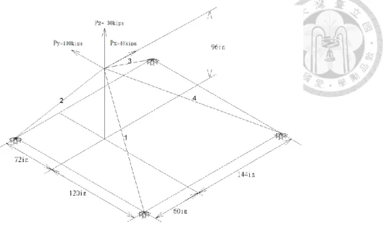
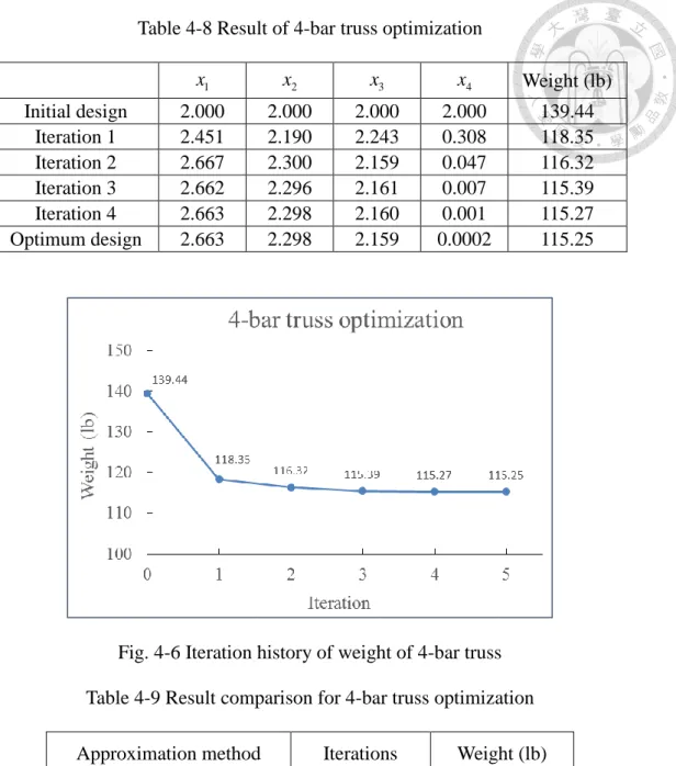
4.3 4-bar truss optimization ... 35

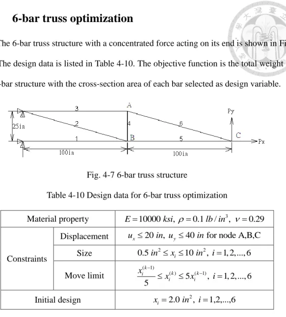
4.4 6-bar truss optimization ... 38

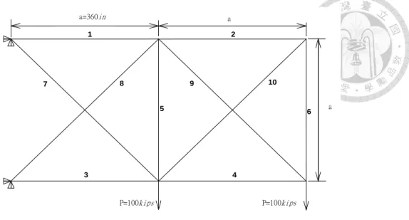
4.5 10-bar truss optimization ... 39

4.6 25-bar truss optimization ... 41

4.7 Multi-section circular beam optimization ... 44

4.8 Multi-section tube beam optimization ... 46

4.9 Multi-section rectangular beam optimization ... 48

Chapter 5 Optimization of large scale structures ... 50

5.1 Effective finite element model construction for PCB ... 50

5.1.1 Material property identification for orthotropic thin plate ... 51

5.1.2 Effective FE model construction for PCB ... 55

5.2 Optimization of high-accuracy measuring stage ... 59

5.2.1 Optimization of gantry ... 59

5.2.2 Optimization of modified gantry ... 63

5.2.3 Optimization of y-stage ... 67

Chapter 6 Conclusion and suggestion ... 72

6.1 Conclusion ... 72

6.2 Suggestion ... 72

REFERENCES ... 74

Appendix: User manual of integrated optimization program ... 77

A.1 Program setting ... 77

A.2 Operation step ... 79

Vitae ... 80

LIST OF FIGURES

Fig. 2-1 Flow chart of developed optimization program ... 19

Fig. 3-1 Approximate functions with different orders ... 20

Fig. 3-2 Functions of MISE with p  ... 22 _i 1 Fig. 3-3 Functions of MISE with p  ... 23 _i 1 Fig. 3-4 Functions of MISE with different exponents ... 25

Fig. 3-5 Piecewise approximate function of TPPAA ... 26

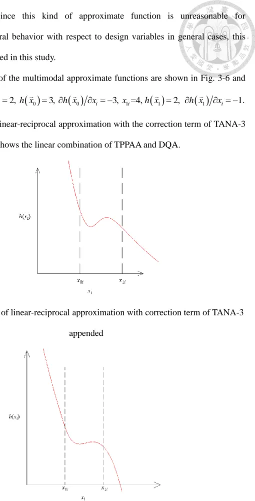
Fig. 3-6 Illustration of linear-reciprocal approximation with correction term of TANA-3 appended ... 30

Fig. 3-7 Illustration of linear combination of TPPAA and DQA ... 30

Fig. 4-1 2-bar truss structure ... 32

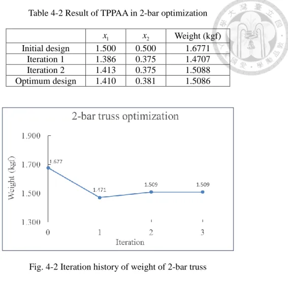
Fig. 4-2 Iteration history of weight of 2-bar truss ... 33

Fig. 4-3 3-bar truss structure ... 34

Fig. 4-4 Iteration history of weight of 3-bar truss ... 35

Fig. 4-5 4-bar truss structure ... 36

Fig. 4-6 Iteration history of weight of 4-bar truss ... 37

Fig. 4-7 6-bar truss structure ... 38

Fig. 4-8 Iteration history of weight of 6-bar truss ... 39

Fig. 4-9 10-bar truss structure ... 40

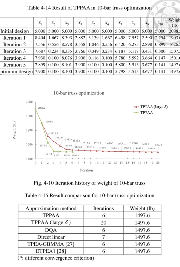
Fig. 4-10 Iteration history of weight of 10-bar truss ... 41

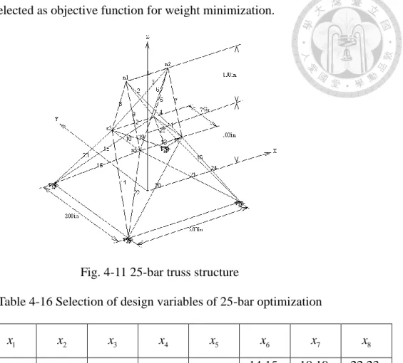
Fig. 4-11 25-bar truss structure ... 42

Fig. 4-12 Iteration history of weight of 25-bar truss ... 43

Fig. 4-13 Multi-section circular beam structure ... 44

Fig. 4-14 Iteration history of weight of multi-section circular beam ... 45

Fig. 4-15 Multi-section tube beam structure ... 46

Fig. 4-16 Iteration history of weight of multi-section tube beam ... 47

Fig. 4-17 Multi-section rectangular beam structure ... 48

Fig. 4-18 Iteration history for multi-section rectangular beam ... 49

Fig. 5-1 CAD model of the thin plate ... 51

Fig. 5-2 Meshed FE model of thin plate ... 52

Fig. 5-3 Meshed FE model of PCB ... 55

Fig. 5-4 Boundary conditions for EMA of PCB ... 55

Fig. 5-5 FRF of PCB by EMA ... 56

Fig. 5-6 High-accuracy measuring stage for wafer inspection ... 59

Fig. 5-7 Selection of design variables for gantry... 60

Fig. 5-8 Boundary condition of gantry in FEA ... 60

Fig. 5-9 Iteration history of weight of gantry ... 62

Fig. 5-10 Selection of design variables for modified gantry ... 64

Fig. 5-11 Meshed FE model of modified gantry ... 64

Fig. 5-12 Iteration history of weight of modified gantry in case A ... 66

Fig. 5-13 Iteration history of weight of modified gantry in case B ... 67

Fig. 5-14 Simplified parametric CAD model of y-stage ... 68

Fig. 5-15 Selection of design variable for y-stage ... 68

Fig. 5-16 Meshed model of y-stage ... 68

Fig. 5-17 Iteration history of weight of y-stage ... 71

Fig. A-1 Operation steps of the optimization program ... 79

LIST OF TABLES

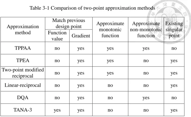
Table 3-1 Comparison of two-point approximation methods ... 28

Table 4-1 Design data for 2-bar truss optimization ... 32

Table 4-2 Result of TPPAA in 2-bar optimization ... 33

Table 4-3 Result comparison for 2-bar truss optimization ... 33

Table 4-4 Design data for 3-bar truss optimization ... 34

Table 4-5 Result of TPPAA in 3-bar truss optimization ... 35

Table 4-6 Result comparison for 3-bar truss optimization ... 35

Table 4-7 Design data for 4-bar truss optimization ... 36

Table 4-8 Result of 4-bar truss optimization ... 37

Table 4-9 Result comparison for 4-bar truss optimization ... 37

Table 4-10 Design data for 6-bar truss optimization ... 38

Table 4-11 Result of TPPAA in 6-bar truss optimization ... 39

Table 4-12 Result comparison for 6-bar truss optimization ... 39

Table 4-13 Design data for 10-bar truss optimization ... 40

Table 4-14 Result of TPPAA in 10-bar truss optimization ... 41

Table 4-15 Result comparison for 10-bar truss optimization ... 41

Table 4-16 Selection of design variables of 25-bar optimization ... 42

Table 4-17 Design data for 25-bar truss optimization ... 42

Table 4-18 Result of TPPAA in 25-bar optimization ... 43

Table 4-19 Result comparison for 25-bar optimization ... 44

Table 4-20 Design data for multi-section circular beam optimization ... 44

Table 4-21 Result of TPPAA in multi-section circular beam optimization ... 45

Table 4-22 Result comparison for multi-section circular beam optimization ... 45

Table 4-23 Design data for multi-section tube beam optimization ... 46

Table 4-24 Result of TPPAA in multi-section tube beam optimization ... 47

Table 4-25 Result comparison for multi-section tube beam optimization ... 47

Table 4-26 Design data for multi-section rectangular beam optimization ... 48

Table 4-27 Result of TPPAA in multi-section rectangular beam optimization ... 49

Table 4-28 Result of multi-section rectangular beam ... 49

Table 5-1 Material property of the thin plate ... 52

Table 5-2 Natural frequencies of the thin plate ... 52

Table 5-3 Selection of design variables for fitting the frequencies of the thin plate ... 53

Table 5-4 Design data for fitting natural frequencies of the thin plate ... 53

Table 5-5 Result of natural frequencies after fitting ... 54

Table 5-6 Obtained elastic constants by fitting natural frequencies ... 54

Table 5-7 Result of TPPAA in elastic constants identification of the thin plate ... 54

Table 5-8 EMA result of PCB ... 56

Table 5-9 Selection of design variables for fitting natural frequencies of the PCB ... 56

Table 5-10 Material properties of PCB ... 57

Table 5-11 Design data for effective FE model ... 57

Table 5-12 Comparison of natural frequencies between effective model and EMA result58 Table 5-13 SAO result with TPPAA for PCB FE model construction ... 58

Table 5-14 Result comparison with different approximation methods ... 58

Table 5-15 Material property of gantry ... 60

Table 5-16 Design data of gantry optimization ... 61

Table 5-17 Result of TPPAA for gantry optimization in case A ... 61

Table 5-18 Result of TPPAA for gantry optimization in case B ... 62

Table 5-19 Result of TPPAA for gantry optimization in case C ... 62

Table 5-20 Result comparison of gantry optimization in case A ... 63

Table 5-21 Result comparison of gantry optimization in case B ... 63

Table 5-22 Result comparison of gantry optimization in case C ... 63

Table 5-23 Design data of modified gantry optimization ... 65

Table 5-24 Result of TPPAA for modified gantry optimization in case A ... 66

Table 5-25 Result of TPPAA for modified gantry optimization in case B ... 66

Table 5-26 Result comparison of modified gantry optimization in case A ... 67

Table 5-27 Result comparison of modified gantry optimization in case B ... 67

Table 5-28 Material property of y-stage ... 69

Table 5-29 Design data of y-stage optimization ... 69

Table 5-30 Result of TPPAA for y-stage optimization in case A ... 70

Table 5-31 Result of TPPAA for y-stage optimization in case B ... 70

Table 5-32 Result of TPPAA for y-stage optimization in case C ... 70

Table 5-33 Result comparison of y-stage optimization in case A ... 71

Table 5-34 Result comparison of y-stage optimization in case B ... 71

Table 5-35 Result comparison of y-stage optimization in case C ... 71

LIST OF SYMBOLS

E Elastic modulus

 

h x Original function to be approximated

 

h x Function value at the current design point

 

h x Function value at the previous design point n Number of design variables

n b Number of behavior constraints n c Number of constraints

n s Number of size constraints

x 0i The i-th design variable at the current design point x 1i The i-th design variable at the previous design point

x i The i-th design variable x Design variable vector

x 0 Design variable vector of the current design point x 1 Design variable vector of the previous design point

 ^k

xi The i-th design variable in k-th iteration

 The given number for criterion of adoption of substitute function

 Poisson’s ratio

 Density

 i Stress in the i-th element

Chapter 1 Introduction

In this chapter, the history of structural optimization and the development of approximation methods are briefly introduced first. Then, the outline of the thesis is presented.

1.1 Introduction to structural optimization

Structural optimization has been developed more than a century. The main purpose of structural optimization is to improve the design under specific restrictions.

Conventionally, design improvement relies on the engineer’s experience with trial and error. It costs considerable time and may not obtain the optimal result. Nowadays, automated structural design is available with integrating well developed finite element analysis software and optimization theory. It can find the optimum design with less subjective judgement.

With the development of finite element method, structural analysis is no longer limited to the theoretical derivation. However, it takes considerable time for the large and complicate structures. In order to save the time of design process, approximation technique is introduced.

Approximation methods converts the implicit structural functions into explicit ones to generate the sub-problems, which can be solved with mathematical optimization. It saves much efforts by reducing the number of repeated finite element analyses.

Local approximation schemes construct approximated functions from the response and the sensitivities of a design point. Hence the problem with implicit structural behavior can be transformed into a mathematical problem with explicit functions with the approximation reliable around the design point. After solving sequential sub-problems, the optimal solution can be found after the process converging. This

technique is also known as sequential approximate optimization (SAO).

For the less finite element analyses in SAO process, the choice of the approximation scheme is better to depend on the characteristics of the problem. For instance, in simple truss problems with design variables of cross section area, direct linear approximation is the best for total weight of truss, reciprocal approximation is more appropriate for stress and displacement. However, for the complicate cases, it is still hard to determine the most suitable scheme. In spite of that, some principles of approximation may be held to ensure the approximation quality for general cases.

1.2 Paper review

In 1904, Michell calculated the theoretical lower bound of the weight of truss structures with stress constraints [1]. The theoretical derivation of ideal structures was an important inspiration for structural optimization. After finite element method was proposed and developed maturely, structural optimization is valid for designing complicate structures.

In 1974, Schmit and Farshi applied approximation concepts to convert structural behavior into explicit functions of design variables [2]. This method turned limited information from structural analyses into simple approximate functions, and greatly reduced the time of structural optimization process.

So far, a lot of local approximation methods have been developed. Among these schemes, direct linear approximation is the most fundamental approach which performs the 1st order Taylor series expansion in terms of design variables. However, most structural characteristics are nonlinear, this method may not be reliable for therefore. To enhance the approximation quality, some scholars proposed reciprocal approximation method, which adopting the reciprocals of original variables as intervening variables in

1st order Taylor series expansion [3]. This approximation method is quite suitable for stress and displacement constraint in simple truss problems when cross-section area is selected as design variable. However, the function value tends to infinity when the design variable approach zero that may cause inappropriate approximation. To overcome this problem, Haftka and Shore proposed modified reciprocal approximation method to shift the singular point in reciprocal approximation [4]. In 1979, Starnes and Haftka proposed conservative approximation method [5] which is also known as convex linearization (COLIN) presented by Fleury and Braibant [6]. This method adopts either direct linear or reciprocal approximation for each design variable, according to which approximate function is estimated higher. In other words, conservative approximation adopts the more conservative one between direct linear and reciprocal approximation for every design variable. In 1987, Svanberg presented the method of moving asymptotes (MMA), which can be regarded as the generalization of CONLIN [7].

To improve the approximation quality of single-point approximations, a lot of approximation schemes developed subsequently with utilizing the information of previous design point to construct approximate functions. These approximations are classified as two-point approximations. In 1987, Haftka et al. proposed two-point modified reciprocal approximation which has the strategy to decide the indeterminate coefficients in modified reciprocal approximation [8]. However, this strategy is undefined when the derivatives of two successive points have the different signs. In 1990, Fadel et al. proposed two-point exponential approximation (TPEA) [9]. TPEA performs Taylor series expansion with exponential intervening variables. The derivative of the previous design point is used to determine the exponent. But this approximation lacks definition for two-point approximation when the derivatives of the variable of two successive points have the different signs. In 1994 and 1995, Wang and Grandhi

proposed a series of two-point adaptive nonlinear approximations (TANA) based on TPEA, which enhance TPEA by matching the function value of previous design point [10][11]. In 1994, Snyman and Stander presented spherical approximation method (SAM) which appends a quadratic term to direct linear approximation for correcting the function value of the previous design point [12]. In 1995, Fadel classified the approximate functions into monotonic and non-monotonic functions [13]. It is suggested that the selection the approximations should consider the characteristic of monotonicity of the structural behavior. Then the mixed method is proposed named DQA-GMMA, which adopts monotonic approximation for design variable when the derivatives of two successive design points have the same signs, and vice versa.

In 1997, Zhang and Fleury proposed modified convex approximation (MCA) based on CONLIN [14]. MCA increases the convexity of approximation to avoid non-convergent process. In 1998, Xu and Grandhi proposed two-point adaptive nonlinear approximation-3 (TANA-3), which appends a term to TPEA for additionally matching the function value of previous design point [15]. In 2000, Xu et al. presented a new two-point approximation approach which uses the linear combination of linear and reciprocal approximations to match the derivatives of previous design point [16]. In 2001, Kim et al. presented two-point diagonal quadratic approximation (TDQA) based on TPEA [17]. TDQA adds shifting level into exponential intervening variables to avoid the singularity of the derivatives. In 1996, Chickermane and Gea proposed generalized convex approximation (GCA) [18]. GCA uses the derivatives of two points to construct approximate functions without lacking definition in TPEA. In 2007, Groenwold proposed incomplete series expansion (ISE) which includes a series of approximations [19]. ISE uses quadratic, cubic, and even higher order diagonal terms to construct the approximate functions.

Several approximation schemes have the approximate function convex to ensure stability of the optimization process such as GCMMA [20][21]. In 2015, Li proposed an adaptive quadratic approximation (AQA) which enforces the approximate functions to be strictly convex to improve the robustness and convergence performance of the optimization process [22]. However, this enforcement would cause inconsistency and may lower the efficiency of optimization process.

Moreover, Chiou proposed two new convex approximation methods in 2000, including self-adjusted convex approximation (SACA) and two-point convex approximation (TPCA) [23]. In 2002, Chen proposed improved two-point approximation (ITPA) which can be seen as the combination the linear-reciprocal and TPEA [24]. In 2007, Chang proposed quasi-quadratic two-point conservative approximation (QTCA) [25]. In 2010, Chen proposed exponential MMA (EMMA), which makes the order of intervening variables in MMA adjustable for more flexibility [26]. In 2012, Chen proposed a new mixed two-point approximation method which is the combination of TPEA and GBMMA [27]. In 2013, Jiang proposed enhanced two-point exponential approximation (ETPEA) to conquer the problem of lack of definition in TPEA [28]. ETPEA use intervening variable which is the second order Taylor series expansion of the original variable to deduce the new formula as the remedy of TPEA.

1.3 Strategies of research

The approximation quality is the crucial factor for the efficiency and stability in SAO process. This thesis presents a new approximation method, named two-point piecewise adaptive approximation (TPPAA). TPPAA is applied to construct the approximate functions of structural behavior such as stress, displacement and natural

frequency for optimization problems. The strategies are as follows:

(1) Review the existing approximation schemes and discuss the merits and defects of each method.

(2) Test some classical approximation methods in several optimization problems and compare the approximation quality in each case.

(3) Create the 1-D plot of the approximate functions in several cases to realize the characteristics of each approximation.

(4) The new method is developed and tested in several optimization problems to verify its practicability.

1.4 Outline

There are six chapter in this thesis:

Chapter 1: Introduce the development of structural optimization and the existing approximation methods briefly. After that, the research strategy of this study is mentioned.

Chapter 2: Introduce the procedure of mathematical optimization in this study and several existing approximation methods.

Chapter 3: Present the derivation of new approximation method developed in this study. Also the characteristics of the new method is compared with other approximation methods.

Chapter 4: Apply the proposed approximation method to several small scale structures and compare the results with other approximation methods.

Chapter 5: Apply the proposed approximation method to several large scale structures and compare the results with other approximation methods.

Chapter 6: Conclude the achievements and recommend the future work.

Chapter 2 Application of approximation methods in structural optimization

First, the procedure of mathematical optimization in this thesis is introduced, then several previous approximation methods are also discussed for the development of new approximation method.

2.1 Procedure of mathematical optimization

This section introduces the details of the mathematical optimization in sequence.

The optimization problem can be written as

 

 

Find ,

such that min,

subject to _i 0, 1, 2..., _c, x

F x

g x i n



 

(2.1)

where x denotes the design vector, F x denotes the objective function to be

 

minimized, g x denotes the i-th constraint, i

 

2.1.1 Selection of design variables

The first step for optimization is defining the design variables for the problem.

With taking efficiency in consideration, an optimization problem should prevent from having too many design variables. In order to reduce the design space, one of the solutions is to choose the dominant variables only instead of all the possible ones.

Another way is to link the design variables, which can be expressed as

 

x T X (2.2)

where X denotes the basis of original design vector, x is the reduced basis, and

 

is the connectivity matrix of design variables.

2.1.2 Defining objective function

In this study, the mathematical optimization problem is defined to minimize the objective function as the expression of Eq. (2.1). To deal with the maximization case, from another point of view, the problem is turned into minimizing the negative of the original objective function.

For the problem considering various objective functions, they are linked with appropriate weighted coefficients. It can be written as

   

1 i i ,

i

F x w F x







where F x denotes the total objective function,

 

 

objective function and w denotes the weighted coefficient. _i

2.1.3 Sensitivity analysis

Thanks to well-developed finite element method, the complicate structural analysis is available for optimization nowadays. Besides the response magnitude of structural behavior, the first order derivative, which also called sensitivity, is also required in the local approximation schemes and most search direction algorithms.

Sensitivity analysis is the way to realize the variation tendency of structural behavior with respect to design variables. In this study, backward difference method is adopted in sensitivity analysis, which can be expressed as

 

  



i ,

i i

h x h x h x x

x x

   

   (2.4)

where h x

 

i i

x x

   represents that only the i-th design variable has a small variation  . x_i

2.1.4 Treatment of constraints

In structural optimizations, there are many kinds of constraints, such as stress, displacement, natural frequency, size, and move limit constraints. For the sake of making the mathematical problem in the form as Eq. (2.1), and reducing the influences of numerical difference between different constraints, the constraints should be modified as follows.

A. Behavior constraint

To avoid the fracture of structures or large displacement which influences the performance of structures, stress and displacement constraints are often needed in structural optimizations. These two constraints can be expressed as

, 1, 2,..., , 0, 0,

L U

i i i b

L U

i i

g g g i n

g g

  

  (2.5)

where g_i^L and g_i^U denote the lower and upper bound of the i-th constraint respectively, and n denotes the number of behavior constraints. The constraints _b should be treated as

1.0, if 0

1, 2,..., , 1.0, if 0

i U i M i

i b

i L i i

g g

g g i n

g g

g

  

 

  



(2.6)

where g_i^M denotes the modified constraints.

Moreover, to avoid resonance occurring, the natural frequencies of the structure are often restricted in certain region. The constraint of frequency can be expressed as

, 1, 2,..., , 0.

L

i i b

L i

g g i n

g

 

 (2.7)

The constraints should be treated as

1.0 , 1, 2,..., .

M i

i L b

i

g g i n

 g  (2.8)

B. Size constraint

Size constraints are the limits of design variables due to material specifications, practical demands, and so on. Size constraints can be expressed as

, 1, 2,..., ,

L U

i i i s

D  x D i n (2.9)

where D_i^L and D_i^U denote the lower and upper bounds of allowable sizes respectively, and n denote the number of size constraints. _s

C. Move limit

In the local approximation, approximation is trustable only around the current design point. Hence move limit is introduced, which can be expressed as

, 1, 2,..., ,

L U

i i i

x x x i n

      (2.10)

where  denotes the variation of the i-th design variable, x_i x_i^L and x^U_i are lower and upper bound of the variations of the i-th design variable respectively and n denotes the number of design variables.

2.1.5 Application of approximation methods

Once the mathematical problem is defined, the optimal solution can be found by mathematical programming. However, the relation between structural behavior and design variables is implicit usually. Hence the approximation technique is applied to convert the implicit behavior into explicit functions. Because the approximated functions are constructed by current design point, the formed mathematical problem is not exactly the same as the real problem, but reliable near the current design point. So, to obtain the optimal solution, it requires to solve several optimization problems of approximated functions. Each sub-problem takes the optimal solution of last iteration as

the initial design. This gradual improvement process is known as sequential approximate optimization (SAO).

2.1.6 Application of mathematical optimization

Numerical optimization method can be classified into direct and indirect methods.

Direct method such as method of feasible direction is to solve the optimization problems without transferring the constraints. Indirect method converts the constraints to a part of objective function, hence the constrained problems can be transferred to unconstrained problems.

Indirect method includes interior penalty method and exterior penalty method.

When interior penalty method is adopted, the initial design must be in the feasible domain. However, it cannot guarantee that the initial design is always in the feasible domain in iterative process. So, exterior penalty method is adopted to deal with the constrained problems to make the process valid with infeasible initial design in this study. After transformation, the objective function can be expressed as

2 1

( , ) ( ) ( ) ,

( ), ( ) 0

( ) ,

0, ( ) 0

nc

i j

i i

i

i

x r F x r g x

g x if g x

g x if g x



    

 

   



(2.11)

where ( , )x r denotes the penalized objective function, F x is the objective ( ) function, r is the penalty factor and g x denotes the i-th constraint function. _i( )

2.2 Single-point approximation methods

Single-point approximation methods use the function value and derivatives of single design point to construct the approximate function. Several existing single-point approximation methods are compared in this section.

2.2.1 Direct linear approximation

This approximation method takes the first order Taylor expansion at the current design point. It is the most fundamental method of local approximation. If h x ( ) denotes the function to be approximated, this approximation can be written as

 

0 0

1

( ) ( ) ( ),

n

l i i

i i

h x h x h x x x

 x

   



where h x denotes the approximate function of direct linear approximation, _l( ) x ₀ denotes the variable vector of current point with i-th component x . _0i

Since most behavior functions of general structures are nonlinear, this method may be not reliable.

2.2.2 Reciprocal approximation

The cross-section area of beams and the thickness of plates are often selected as the design variables, and the stress, displacement are often selected as constraints in structural optimization problems. In this kind of problem, the relation between the reciprocals of variables and the constraints are near linear for simple structures. Hence, in this case, performing 1st order Taylor series expansion in terms of reciprocals of the design variables would has the better approximation quality in comparison with direct linear approximation, which is called reciprocal approximation method [3].

 

0 0

1

( ) ( ) ( )( ),

n

i

r i i

i i i

h x x

h x h x x x

x x



   



where h x denotes the approximate function of reciprocal approximation. _r( )

However, x  is the singular point in this approximation method. When the _i 0 design variable approaches to the singular point, the magnitude of the function value and derivative tend to infinity, and the approximation quality would be affected

therefore.

2.2.3 Modified reciprocal approximation

In order to conquer the defect of reciprocal approximation, Haftka proposed modified reciprocal approximation method [4]. The singular point is shifted to enlarge the reliable region. This approximation can be expressed as

 

0 0

1

( ) ( ) ( )( ),

n

i mi

mr i i

i i i mi

h x x x

h x h x x x

x x x



 

  

 



where h_mr( )x denotes the approximate function of modified reciprocal approximation.

The singular point is shifted from zero to x_mi. But the determination of x needs to _mi depend on experience.

2.2.4 Conservative and convex approximation

Conservative approximation selects the more conservative one between direct linear and reciprocal approximations for each design variable [5][6]. So it can ensure that the function value would not less than neither direct linear nor reciprocal approximation. The idea of increasing the conservativeness is to make the solution of approximate problem satisfies the constraints more possible. The formula can be written as

 

 

0 0 0

1 1

( ) ( ) ( ) ( ) ⁱ ,

c i i i i

i i i i i

h x h x x

h x h x x x x x

x x x

 

 

   

 





where h x denotes the approximate function of convex approximation method, _c( )

1 i





1 i





However, the too conservative approximation would reduce the convergence rate and result in low efficiency to the process.

2.3 Two-point approximation

Besides using the response value and sensitivity of current design, two-point approximation methods utilize the information of previous design point to improve approximation quality. Several existing two-point approximation methods are compared in this section.

2.3.1 Two-point modified reciprocal approximation

In 1987, Haftka proposed two-point modified reciprocal approximation method [8], which gives a recommendation on determining the indeterminate coefficient in modified reciprocal approximation method. So these two approximation methods have the same form.

 

0 0

1

( ) ( ) ( )( ),

n

i mi

tmr i i

i i i mi

h x x x

h x h x x x

x x x



 

  

 



where h_tmr( )x denotes the approximate function of two-point modified reciprocal approximation and x denotes the variable vector of previous design point. ₁ x is _mi determined by matching the previous derivative and can be derived as

 

 

0 1

, .

1

i i i

mi i

i i

i

h x h x

x x

x x x

 



 

  

 

 (2.17)

Obviously, it is undefined when the two derivatives have the different signs.

Moreover, x is required to be a positive number to avoid the function value tending _mi infinity, but it is not guaranteed in this method.

2.3.2 Two-point exponential approximation

In 1990, Fadel proposed two-point exponential approximation (TPEA) [9]. It takes

pi

xi as the intervening variable for the first order Taylor series expansion.

   

 





1

,

i

i i

n p

p p

i

tpea i i

i i i

h x x

h x h x x x

x p





   



where h_tpea( )x denotes the approximate function of TPEA. p is determined by fitting _i the derivative of the previous design point.

   

 

1 0

1 0

ln

1 .

ln

i i

i

i i

h x h x

x x

p x x

 

 

   

 

  (2.19)

However, this calculation lacks of definition under following two conditions:

 

 

1 0

0 or _{i i} 0.

i i

h x h x

x x

x x

 

 

  (2.20)

When p cannot be calculated by matching the derivative, direct linear _i approximation is adopted instead. Besides that, p should be restricted in a specified _i range p^L p_i  p^U to avoid inappropriate approximation and p^L  1, p^U  is 1 suggested by the author. When p is larger than _i p with calculated from Eq. (2.19), ^U

U

pi  p is adopted, and vice versa.

The approximate function of TPEA is always monotonic. However, non-monotonic approximation functions are required when the two derivatives of two successive design points have the different signs. Moreover, TPEA has the defect of singularity as reciprocal approximation when p  . _i 1

2.3.3 Linear-reciprocal approximation

In 2000, Xu presented linear-reciprocal approximation method [16]. With the linear combination of direct linear and reciprocal approximation methods, the derivative of the previous design point is matched.

   



 



1 1

,

n n

i

lr i i i i i i

i i i

h x h x x x x x x

  x

 

 





where h x denotes the approximate function of linear-reciprocal approximation. The _lr( ) coefficients  and _i  are determined by matching the gradient of previous design _i point.

 

 

, 1

i i

i

i i

h x h x

x x

x x



 

  

  

  

 

(2.22)

 

i i.

i

h x

 ^ x 

 (2.23)

This method implies that with utilizing the linear combination of two different single-point approximations, a new two-point approximation method which matches the gradient of previous design point can be created arbitrarily.

2.3.4 Incomplete series expansion

In 2007, Groenwold proposed a series of approximations named incomplete series expansion (ISE) [19]. The fundamental idea of ISE is to approximate the Hessian matrix by excluding the off-diagonal terms for saving the computational requirements. The general form can be written as

 

0 0 0

1 2 1

( ) ( ) ( ) ,

n p n

j

ise i i ji i i

i i j i

h x h x h x x x c x x

 x  

     





where h_ise( )x denotes the approximate function of ISE.

The simplest approximate form of ISE family is non-spherical quadratic ISE, which can be expressed as

 

2 0 0 2 0

1 1

( ) ( ) ( ) ,

n n

i i i i i

i i

h x h x h x x x c x x

 x

 

     





where h_2( )x denotes the approximate function of non-spherical quadratic ISE. This approximation method is the same as diagonal quadratic approximation (DQA) [13].

The coefficients are determined by matching the gradient of previous design point.

   

 

1 0

2

1 0

2 .

i i

i

i i

h x h x

x x

c x x

 

  

 

(2.26)

Another member of ISE named non-spherical cubic approximation which can additionally match the function value of previous point with c_2i c₂, i1, 2,...,n.

 

0 0 2 0 3 0

1 1 1

( ) ( ) ( ) ,

n n n

nsc i i i i i i i

i i i i

h x h x h x x x c x x c x x

 x  

       



 

where h_nsc( )x denotes the approximate function of non-spherical cubic approximation.

In conclusion, ISE proposed a way to match extra information with arbitrary approximation forms. An approximate function can fit the derivative of another point by adding a non-spherical term and fit the extra function value by adding a spherical term.

However, all the approximation functions of ISE are the non-monotonic form. Hence it is not appropriate to be applied to some structural behavior since their characteristics of monotonicity.

2.3.5 Two-point adaptive nonlinearity approximation-3

In 1998, Xu and Grandhi proposed two-point adaptive nonlinearity approximation-3 (TANA-3) [15], which appends a correction term to TPEA for matching the function value at previous design point.

 

tana3 0 0 0

1 1

( ) ( ) ( ) 1 ( ) ( ) ,

2

i

i i i i

n p n

p p p p

i

i i i i

i i i i

h x x

h x h x x x x x x

x p^ 

 

     





where h_tana3( )x denotes the approximate function of TANA-3. ₀ ²

1

1 ( ) ( )

2

i i

n

p p

i i

i

x x x







the appended correction term to TPEA, and ( )x can be expressed as

0

2 2

1 0

1 1

1 0

1 0 1 0

1

( ) ,

( ) ( )

2 ( ) ( ) ( ) .

i i i i

i

i i

n n

p p p p

i i i i

i i

n p

p p

i

i i

i i x i

x K

x x x x

x

K h x h x h x x

x p



 





 

   



  

    

        

    



 



(2.29)

The characteristic of the appended term is that the first order derivative equals zero at x and _0i x . So the determination of _1i p is the same as in TPEA, and the same _i inappropriate approximation would encounter in TANA-3.

2.4 Integrated optimization program

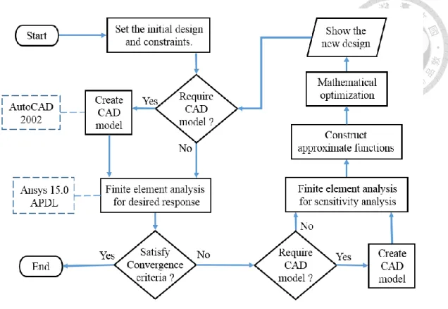
In this study, the automated optimization program is developed in Microsoft Visual C++ 2015 with integrating AutoCAD 2002 and Ansys 15.0 APDL. The flow chart is shown in Fig. 2-1. The procedure is introduced briefly as follow:

(1) Define the optimization problem including design variables, initial design, objective function and constraints.

(2) Output “DesignVariable.lsp” for parametric modeling in AutoCAD 2002 if needed.

The model is output as “model.sat”.

(3) Output “DesignVariable.mac” for finite element analysis in Ansys 15.0 APDL. The results are output in .txt format.

(4) Read the analysis results from .txt files. Then, the approximate functions are constructed to form the sub-problem. The new design is obtained after the mathematical optimization.

Fig. 2-1 Flow chart of developed optimization program

Chapter 3 The proposed approximation method

In this study, a new approximation method is proposed and named two-point piecewise adaptive approximation (TPPAA). Many kinds of structural behavior vary quasi-monotonically with respect to design variables. For this situation, monotonic functions are available in TPPAA when first order derivatives of two successive design points have the same signs. The non-monotonic form can be approximated also when the two first order derivatives have different signs. Moreover, the piecewise approximate functions are adopted to avoid the inappropriate approximation that the existing methods would encounter.

3.1 Modified incomplete series expansion

The fundamental idea of the proposed approximation method is to construct an approximate function of arbitrary order which matched the value of a point and first order derivatives of two points. In other words, it can construct approximate functions with arbitrarily specified nonlinearity degree, as shown in Fig. 3-1.

To avoid confusion, before introducing TPPAA, an approximate function which is based on ISE is discussed first. This new approximation, is named modified incomplete series expansion (MISE), also added the shifting term x for more flexibility and can _mi be expressed as

   

1 1

i ,

n n

p

mise i i mi i

i i

h x h x c x x R

 

 





where h_mise( )x denotes the approximate function of MISE, c x_i, _mi, , p R denote the _{i i} coefficients to be determined. The differential form with respect to i-th variable is expressed as

 

pi

i mi

mise

i i

i i mi

x x

h x

x p c x x



 

  (3.2)

The essential requirement for local approximation is to fit the function value and derivatives at x and it can be achieved by determining ₀ c and _i R as follows with _i arbitrary p and _i x given. _mi

From Eq. (3.2), c can be determined by fitting the derivatives at _i x . ₀

  



0

i .

i mi

i

i p

i i mi

h x x x

c x

p x x

 

 



(3.3)

Then,

1 n

i i

R



0

pi

i i i mi

R c x x (3.4)

can be one of the solution. Hence R is expressed as _i

  



1 .

i i mi

i i

R h x x x

p x

  

 (3.5)

Because MISE is a kind of separable approximation (approximate function consists

of several separable single-variable functions), the approximate function of one variable is discussed for simplicity in the following discussion.

When p  , the approximate function is a non-monotonic function, and _i 1 x is _mi the extreme point, as shown in Fig. 3-2. Hence the sign of second order derivative is based on which side x is with respect to _mi x . Fig. 3-2 shows the approximate _0i functions of MISE which fit a point of x0_i 5, h x

 

 

2, 3

i mi

p  x  is given for h x and 1

 

 

Fig. 3-2 Functions of MISE with p _i 1

When p  , _i 1 x is the singular point, as shown in Fig. 3-3. The magnitude of _mi derivative tends to infinity when the design variable x approaches to _i x . Hence it _mi may cause inappropriate approximation in general cases. Note that in the case of

1, 0

i mi

p   x  , MISE is the same as reciprocal approximation in x  , as shown in _i 0 Eq. (2.13). Fig. 3-3 shows the approximate functions of MISE which fit a point of

   

0_i 5, 0 3, 0 _i 7. _i 0.5, _mi 3

x  h x  h x   x p  x  is given for h x1

 

p  x  is given for ^{h x}

 