軟體評估模式建構技術適用性動態模式之研究(II)

行政院國家科學委員會專題研究計畫 成果報告

軟體評估模式建構技術適用性動態模式之研究(2/2)

計畫類別： 個別型計畫

計畫編號： NSC94-2416-H-011-001-

執行期間： 94 年 08 月 01 日至 95 年 07 月 31 日 執行單位： 國立臺灣科技大學資訊管理系

計畫主持人： 黃世禎

報告類型： 完整報告

處理方式： 本計畫可公開查詢

中 華 民 國 95 年 10 月 16 日

Chinese Abstract

隨著數位與知識經濟時代的來臨，企業相關業務活動對於軟體的依賴日漸加深，使 得軟體的需求也更為多元且複雜。而在這樣的需求環境下，整個軟體開發與維護專案就 更難被掌控來達成特定時程與資源限制下的軟體品質目標。因此，為了要在這樣複雜的 開發環境下依然能達到使用者的要求，軟體組織就必須要能將軟體流程改善與專案管理 的工作深植於整個軟體開發與維護過程中的各個活動上，如此才能真正有效地做好品 質、成本與時程三部分的控管。

而在相關軟體管理活動中，軟體評估模式已經被證明是一個有必要的工具來支援開 發高品質的軟體產品。但在以往的軟體評估研究中，軟體評估模式都是以實體或其屬性 的角度來應用，缺乏對相關軟體評估模式或其建構技術進行較全面性且深入的探討。這 樣往往無法清楚地讓使用者知道這些模式或模式建構技術的使用時機，而容易造成錯誤 的使用，降低了軟體評估模式本身真正的效益。故本研究認為應該要有一套適當且明確 的軟體評估模式適用性之因子架構，來協助軟體專案管理者作為比較相關軟體評估模式 或其建構技術之依據，以便能進行較為客觀、深入且全面性的探討研究，如此便可以瞭 解各模式或其建構技術的使用時機，並提供相關學者或專案管理者可以做出更正確的選 擇與決策。

而為了驗證本架構的實用性，我們也根據本架構中的一個因素–『評估模式中達成 決策所需的評估階段個數』，將軟體評估模式分類成單一階段模式與多重階段模式兩 種，並利用所收集得來的軟體度量資料進行深入的比較，來瞭解其各自的適用時機。與 許多廣為使用的單一階段模式比較下，本研究結果顯示多重階段模式有辦法可以減少收 集評估所需度量資料之工作量；而在精確度上，結果雖然沒有較為優越，卻也在可接受 的範圍內。所以評估者在可接受的評估精確度下，評估者可以使用多重階段模式來減輕 評估時度量值收集的所需工作量。

關鍵詞：軟體評估模式、模式適應性、單一階層模式、多重階層模式、評估模式之精確 度與效率、軟體度量與分析

English Abstract

As enterprises depend heavily on software in all their business activities, software has become increasingly complex and diverse. Hence, it is more difficult to accomplish the designated functions within given constraints (such as cost and schedule) as well as to meet the requirements of high quality software products in software development and maintenance projects. Therefore, an effective software process improvement (SPI) or project management is crucial to the success of software development projects.

Within software-related management activities, software assessment models have been proven as a necessary tool in supporting the fact-based decision making for the development of high quality software. However, most of the existing software-related studies introduced their models or techniques that were only based on the view of software entities and attributes, and this may lack the demonstration of pre-conditions for applying these models or techniques. Hence, this research aims at proposing a factor framework for software experts to compare these models or techniques more objectively, comprehensively and deeply.

In this research, we categorized these models into two types: the one-layered and multi-layered models, in terms of the number of assessment layers required for reaching the decision in an assessment model, which is one of factors in our proposed framework. Then, we compared the assessment accuracy and efficiency for the multi-layered and one-layered models, established from an empirical software measurement dataset. The experimental results showed that the multi-layered model is able to save much effort in collecting all measurement data and can still maintain acceptable assessment accuracy in comparison with the widely used one-layered models. That is, an appraiser may not need to collect all measurement data to reach the required level of assessment accuracy in a particular software process or product assessment problem.

Keywords: Software Assessment Model, One-layered Model, Multi-layered Model;

Assessment Accuracy and Efficiency, Software Measurement and Analysis

Catalog

Chinese Abstract...I English Abstract ... II Catalog ... III

1. Introduction ... 1

2. Literature Reviews ... 2

3. Research Method... 4

4. Experimental Results and Discussions... 12

5. Conclusions ... 16

6. Self-evaluation of This Research Result ... 17

Reference... 17

1. Introduction

As enterprises depend heavily on software in all their business activities, software has become increasingly complex and diverse. Hence, it is more difficult to accomplish the designated functions within given constraints (such as cost and schedule), as well as to meet the requirements of high quality software products in software development and maintenance projects. According to Standish Group’s survey from 9,236 completed worldwide IT projects in the third quarter of 2004, the results showed that 53% of the projects failed to meet the requirements of predefined budget, schedule and functionalities, and 18% were cancelled prior to their completion or delivery [1]. Therefore, effective software process improvement (SPI) or project management is crucial to the success of software development projects.

In order to provide the information needed for all SPI and project management activities, software measurement is required as an integral part of software development process.

Among all software measurement activities, assessing external attributes of three software project entities (product, process, and resource) by means of associated software measures is a common but important activity, since it determines whether a project manager can make objective, consistent and instantaneous decisions. Recently, the topic of software measurement has received increasing attention by both the academia and software industry.

One of the examples is that “Measurement and Analysis (MA)” has become a process area in the maturity level II of Capability Maturity Model Integration (CMMI) from one of common features in the Capability Maturity Model for Software (SW-CMM), both released by Software Engineering Institute (SEI) of Carnegie Mellon University (CMU) [2]. Moreover, the International Organization for Standardizations (ISO) also released the ISO/IEC 15939 [3]

in 2002, which defines a software measurement process for all software-related engineering and management disciplines.

Among various software measurement activities, software process and product assessment is one of the important activities for producing timely and objective information during fact-based decision making process. Since 1998, ISO has released ISO/IEC 14598 series of standards [4] that gives standard methods for software product quality measurement and evaluation; while ISO/IEC 15504 series of standards [5] provides a framework for the assessment of software processes and thus can be used to determine process improvement and process capability.

Of software assessment practices, software process, product classification and rating are very common but particularly important for making the fact-based decisions. Such models have been proven as a necessary tool in supporting the fact-based decision making for the development of high quality software. Thus, during the past decades, a great number of research works in the literature have addressed the problems regarding software-related classification and rating, especially on proposing methods or techniques for establishing software assessment models.

However, most of the existing software-related studies introduced their models or techniques that were only based on the view of software entities and attributes. This may lack the demonstration of pre-conditions for applying these models or their techniques. It is essential for software project managers to determine which assessment model is suitable for their respective objectives. However, this important topic in the software measurement field is not widely addressed in the literature. Hence, this research aims at proposing a factor framework for software experts to compare these models or techniques more objectively, comprehensively and deeply. Furthermore in order to demonstrate the practicability of our proposed framework, we also compare these models, established from an empirical software measurement dataset, based on the factor of “the number of layers required for reaching decision” in our proposed framework.

2. Literature Reviews

Within software MA practices, software process, product classification, and rating are quite common but particularly important for making the fact-based decisions. Thus, over the past decades, a great number of researches in the literature have addressed the problems regarding software-related classification and rating, especially on proposing methods or techniques for establishing software assessment models.

The simplest but most widely adopted method in establishing software assessment models is “decomposition by expert judgment”. The software assessment model established by this method is organized in hierarchically multidimensional structure. One of many examples is a hierarchical model for object-oriented design (OOD) quality assessment proposed by Bansiya and Davis [6]. The OOD quality was assessed as an aggregation of the individual high-level quality attributes of models. The high-level attributes were assessed using a set of empirically identified and weighted object-oriented design properties derived

from object-oriented measures. This OOD quality assessment model is classified as a one-layered assessment model in this study.

As various techniques in other disciplines have been developed, and quantitative software measurement data are available for use, lots of well-known techniques were introduced to address software-related classification problems. These techniques include artificial neural network (ANN) [7-10], Bayesian classifier [11], case-based reasoning (CBR) [12], discriminant analysis (DA) [13-17], decision tree (DT) [18-22], fuzzy classification [23]

and logistic regression (LR) [24-26]. Some studies [27-29] have also integrated more than one technique to building software classification models. Moreover, some studies [30-38]

established software classification models by using the same datasets and performance evaluation indicators for further comparisons of the capabilities of the established models.

Essentially, establishing a software assessment model should consider two important aspects: assessment accuracy and assessment efficiency. Assessment accuracy means that an assessment model can precisely distinguish the specifically measured attribute of a software entity, while assessment efficiency concerns how efficient an appraiser uses the assessment model for his purpose, i.e., the number of used independent variables in an assessment.

In previous software-related classification studies, a widely-used measure of the assessment accuracy is the “misclassification rate of a classification model”. For example, Ebert and Schneidewind [23, 39] utilized the “type II misclassification rate” to choose the assessment model; while Khoshgoftaar and Allen [25, 40] proposed a balance between type I and II misclassification rates according to the specific need of an appraiser. Type II misclassification rate is defined as the proportion of risk-prone cases misclassified as non-risk-prone cases, and type I misclassification rate is just the opposite. In addition to the cost of individual misclassification rate, Khoshgoftaar and Seliya [12] and Khoshgoftaar, Seliya and Herzberg [41] have also individually investigated the use of ‘‘expected cost of misclassification (ECM)’’ and ‘‘modified expected cost of misclassification (MECM)’’ as a singular unified model-evaluation measure to avoid the use of more than two separate measures.

Apart from assessment accuracy, assessment efficiency is also an important factor when deciding a suitable software assessment model. However, there were few software-related literatures mentioning the measures of assessment efficiency for a software assessment model.

One of the few literature works is Esteva [18], who used ID3 algorithm to recognize reusable

software modules, and compared established model with the results given by experts based on the overall misclassification rates and the tree complexity indicators.

Up to now, many diverse techniques have been applied to the software-related classification problems. However, most of the existing software-related studies introduced their models or techniques that were only based on the view of software entities and attributes.

These assessment models established by these techniques can be classified based on different views for the advanced comparison. Therefore, this research aims at proposing a factor framework for software experts to compare these models or techniques more objectively, comprehensively and deeply.

3. Research Method

3.1 Factor Framework for the Adaptability of Software Assessment Models

The main goal of this research is to provide an easily-extensible factor framework for

the adaptability of software assessment models and their associated techniques.

In order to increase the extensibility of our framework and the integrity between its factors, we introduce a rule-based framework for this study. The adopters can effortlessly add new factor without substantially reforming or modifying the antecedent framework and handily form their problems with these factors and logical operators (e.g. “AND” and “OR”

etc.). The proposed factors in this study are described as follows:

z Regarding dependent variables

„ Scale type of the dependent variables: nominal, ordinal, interval, ratio or absolute scales.

„ Amount (nominal and ordinal scales) or Range (the remainder scales) of values in a dependent variable.

„ Vagueness level of the dependent variables.

„ Uncertainty level of the dependent variables.

„ Distribution type of values in the dependent variables: discrete uniform distribution, normal distribution, uniform distribution, etc.

z Regarding independent variables

„ Amount of whole independent variables in a model.

„ Distribution of different types of independent variables in a model.

‹ Based on different scale types of independent variables in a model:

nominal, ordinal, interval, ratio and absolute scales.

‹ Based on different types of value range of independent variables in a model.

‹ Based on different vagueness levels of independent variables in a model.

‹ Based on different uncertainty levels of independent variables in a model.

‹ Based on different distribution types of independent variables in a model:

discrete uniform distribution, normal distribution, uniform distribution, etc.

z Problems with no objective, single objective, multiple non-conflict objectives, or multiple conflict objectives.

z Quality (the ratio of missing data or outliers) and amount of historical data.

z Based on a model, the acceptable levels of assessment accuracy and efficiency for an appraiser.

z Number of assessment layers required for reaching the decision in an assessment model (such as the one-layered comprehensive assessment and the multi-layered iterative assessment).

z The others.

3.2 Comparisons of Multi-Layered and One-Layered Assessment Models Based on Empirical Software Measurement Dataset

In

demonstrate the practicability of this framework and choose a main factor, namely

one-layered and multi-layered software assessment models.

M

ost existing software assessment models are one-layered, which requires all

measurement data available for generating an assessment result; while a multi-layered

software assessment model provides more than one assessment layer for the appraiser

to generate the derived assessment result. That is, such a model allows the appraiser to gradually collect measurement data when performing the assessment. Intuitively, the one-layered assessment model requires more effort in collecting all measurement data than the multi-layered assessment model. On the contrary, the one-layered model applies more complete measurement data for higher possibility to produce better assessment accuracy than the multi-layered model.

However, the assessment activities usually need to be implemented repeatedly throughout the software development life cycle. Meanwhile, the collection of software measurement data is generally strenuous and labor consuming. It is essential for software project managers to determine which assessment model is suitable for their respective objectives, since such a choice would significantly affect the assessment efficiency, namely effort affected by the amount of measurement data to be collected, and the accuracy of the assessment result. Therefore, this study aims at comparing the assessment accuracy and efficiency for the multi-layered and one-layered models.

3.2.1 Research Procedure

The comparison of performance between one-layered and multi-layered assessment models comprises the following four steps.

Step1: Define two types of assessment models and select the criteria for adopted techniques in this study.

1. Define one-layered and multi-layered assessment models

A one-layered assessment model has only one assessment layer, in which all measurement data should be available when performing the assessment. On the contrary, a multi-layered assessment model provides more than one assessment layer for the appraiser to generate the derived assessment result. That is, such a model allows the appraiser to gradually collect measurement data when performing the assessment. If the expected assessment accuracy is achieved, the assessment is then completed. Hence, the appraiser may not need to prepare all measurement data in the first layer of the model, but only collect necessary measurement data at each particular assessment layer.

2. Decide the factors for selecting the modeling techniques

The following three factors are used to choose the modeling techniques for these two assessment models.

(1) The selected techniques should be widely used in software-related classification studies.

(2) The selected techniques should automatically select the appropriate independent variables in the model, so that the efficiency of the assessment models can be objectively compared.

(3) The selected techniques can be found in commercial-off-the-shelf (COTS) software packages, so that researchers and practitioners can easily use these packages for building the models.

Step2: Determine assessment accuracy and efficiency indicators for comparing the performance of these two software assessment models, as shown in Section 3.3.

Step3: Preprocess the empirical software measurement data. The three-fold cross-validation approach, a widely adopted method in the literature [42], was used to establish and validate the models. Project data are randomly arranged into three groups of equal number via stratified sampling, so the proportions of training and test data can be better fitted into the distribution of raw data for more stable and realistic accurate measures. Two groups are used as the training dataset and the remaining group is treated as the test dataset. That is, two-thirds of the project data are used to build the model and one-third is adopted to validate the performance of the established model. The above procedure is repeated three times in different combinations. Then, all test dataset accuracy is aggregated as the test result.

Step4: Establish two types of software assessment models and compare their performances.

The training datasets prepared in step 3 are used to establish two different software assessment models by means of the identified techniques in step 1. Then, the performance of these software assessment models would be respectively computed at the test stages. Finally, experimental results are presented and further discussions and conclusions are accordingly drawn.

3.2.2 The Selected Techniques

According to the identified factors in step 1 of Section 3.1, four classification modeling techniques were determined for establishing two types of software assessment models. The techniques include ANN, DA, DT and LR. The taxonomies and brief descriptions of these four techniques are given as follows.

3.2.2.1 Classification Techniques for Building the One-layered Assessment Model

z Artificial Neural Network (ANN)

An ANN-based software assessment model is presented as a set of interconnected input/output neurons, where each connection has a weight associated with it for simulating bio-learning behaviors in an assessment. Among various types of ANN models, the most known model in previous software-related classification studies is the feed-forward back-propagation ANN (FF-BP ANN). At the training stage, weights are computed by using the feed-forward back-propagation algorithm, which is a form of gradient descent method. In this study, Saha’s FF-BP ANN classifier, written by Excel VBA, was utilized to establish the ANN-based one-layered software assessment model. The more detailed descriptions of FF-BP ANN can be referred to [43].

z Discriminant Analysis (DA)

In previous software-related classification studies, DA is also one of the widely-used methods. Given a set of independent variables, the DA-based software assessment model would attempt to find the suitable linear combination of those variables. This model builds the discriminant functions by using the ordinary least-squares and stepwise methods, as well as the linear regression method. In this study, the DA module in the SPSS package is utilized to build the DA-based one-layered software assessment model with the smallest F ratio stepwise method. The more detailed descriptions on DA can be referred to [44].

z Logistic Regression (LR)

LR is a generalization of the linear regression method with a discrete outcome. Due to such a discrete dependent variable, a LR-based software assessment model cannot be directly established with conventional linear regression approach. Hence, instead of predicting whether the outcome of the dependent variable will occur, the model is built to predict the logarithm of the odds of outcome occurrences based on the maximum likelihood estimation and some variable selection methods. Besides, the LR software assessment model is also popular in that it can enable researchers to overcome several restrictive assumptions of the ordinary least squares (OLS) regression and discriminant analysis methods. In this study, the multi-nominal LR (MNLR) in the SPSS package was adopted to establish the LR-based one-layered software assessment model with the forward entry stepwise method. The more detailed descriptions on MNLR can be referred to [44].

3.2.2.2 Classification Techniques for Building the Multi-layered Assessment Model

z Decision Tree (DT)

Based on the historical data, a DT-based software assessment model is presented as a tree graph or multi-layered rules to classify new unseen cases. It provides various assessment paths or layers for assessors to specially treat each new case. So far, many types of the decision tree algorithms were proposed in the literature. They were also widely introduced in the software-related classification studies. Some examples are C4.5 [21], ID3 [18, 19], SPRINT-SLIQ [22], and TREEDISC [20].

In this study, Quinlan’s C4.5 algorithm of the 8th release (C4.5-R8) [45] was utilized for establishing the DT-based multi-layered software assessment model, as it is well-known in classification studies and can easily handle different splitting problems for the ordinal independent variables. The C4.5-R8 is a descendent of the induction programs: ID3 (Quinlan, 1979) and C4 (Quinlan, 1987) [46]. Its more detailed descriptions on C4.5 can be referred to [46].

3.2.3 Model Performance Indicators

As identified in Step2 of Section 3.1, two indicators are used to compare the performance of one-layered and multi-layered software assessment models. They are the assessment accuracy and assessment efficiency, with detailed descriptions presented as follows.

3.2.3.1 Assessment Accuracy

The measures of overall and partial misclassification rates were widely used indicators in previous software-related classification studies [23, 40], and thus are adopted to evaluate and compare the assessment accuracy of two software assessment models in this study. The lower the misclassification rate, the better the accuracy of the assessment model. Generally, software experts find it hard to determine the misclassified costs (also called the weights) of all classes for integrating partial misclassification rates into overall misclassification rate, especially in the situations with more than two classes. Therefore, equally-weighted overall misclassification rate (EW-OMR) is treated as a measure for selecting the best training model as shown in Eq. (1).

data entire of

Number

cases ied

misclassif of

Number OMR

-

EW = ...(1)

The other adopted assessment accuracy measure in this study is the partial

misclassification rates, which can be divided into Type I and Type II misclassification rates (Type I MR and Type II MR) for a two-classed dependent variable. The formulas are defined as Eqs. (2) and (3).

cases prone

- risk - non total of Number

cases prone

- risk - non ied misclassif of

Number MR

I

Type =

... (2)

cases prone

- risk total of Number

cases prone

- risk ied misclassif of

Number MR

II

Type =

... (3)

3.2.3.2. Assessment Efficiency

Three measures for comparing the assessment efficiency of two software assessment models are used in this study. These are “the total number of uniquely used variables in an assessment model” (TNoUVarsM), “the average number of used variables within all assessment paths” (ANoUVarsAP), and “the number of uniquely used variables in the longest assessment path” (NoUVarsLAP). The TNoUVarsM measures the variable utility of an assessment model. The ANoUVarsAP and NoUVarsLAP depict the average and worst assessment efficiencies of respective assessment model. It is noted that an assessment path represents a complete assessment, and the longest assessment path refers to the maximal number of the uniquely used variables in a model to finish a complete assessment. The formula of ANoUVarsAP is defined as Eq. (4).

model a in paths assessment of

Number

paths assessment all

within variable

used of number Aggregated

ANoUVarsAP=

... (4)

3.2.4 An Empirical Software Measurement Dataset

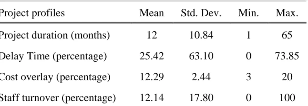
An empirical software measurement dataset, comprising 115 historical software projects [47], were adopted in this study. The profiles of this dataset are summarized in Table 1. The dependent variable is “whether the project is cost risk-prone or non-risk-prone”. The cost risk is defined as if the final product of a software project can be delivered within budget. The proportion of the cost risk-prone projects is 28.7%. The value of the cost risk-prone project class is given as 1, and the value of the risk non-risk-prone project class is given as 2.

Table 1: Profiles of the collected 115 software projects Project profiles Mean Std. Dev. Min. Max.

Project duration (months) 12 10.84 1 65 Delay Time (percentage) 25.42 63.10 0 73.85 Cost overlay (percentage) 12.29 2.44 3 20 Staff turnover (percentage) 12.14 17.80 0 100

The independent variables in this study include 27 risk factors, which are classified into six dimensions. Each of them presents an exposure to an individual risk factor, which is defined as its impact on the project cost multiplied by its occurrence frequency. The measurement scale for the impact of an individual risk factor on the project cost has five levels - minimal or no impact (value=1), <5% (value=2), 5-7% (value=3), 7-10% (value=4) and >10% (value=5); while the measurement scale for the occurrence frequency of an individual risk factor also has five levels - remote (value=1), unlikely (value=2), likely (value=3), highly likely (value=4) and near certainty (value=5). The profiles of the 27 independent variables are shown in Table 2.

Table 2: Profiles of the 27 risk factors within the collected 115 software projects Risk factors grouped by six dimensions Mean Std.

Dev. Min. Max.

Organizational environment risks

1. Change in organizational management during the project 6.16 5.62 1 25 2. Corporate politics with negative effect on project 6.97 6.42 1 25

3. Unstable organizational environment 5.25 5.62 1 25

4. Organization undergoing restructuring during the project 4.75 5.29 1 25 User risks

5. Users resistant to change 6.21 4.41 1 20

6. Conflict between users 6.34 5.11 1 20

7. Users with negative attitudes toward the project 5.32 5.57 1 25

8. Users not committed to the project 6.03 5.04 1 25

9. Lack of cooperation from users 5.83 5.03 1 25

Requirements risks

10. Continually changing system requirements 11.27 7.07 1 25 11 .System requirements not adequately identified 8.89 6.68 1 25

12. Unclear system requirements 8.68 7.06 1 25

13. Incorrect system requirements 7.57 7.07 1 25 Project complexity risks

14. Project involved the use of new technology 7.44 5.84 1 25

15. High level of technical complexity 6.82 5.57 1 25

16. Immature technology 5.33 5.53 1 25

17. Project involves use of technology that has not been used in

prior projects 7.18 6.47 1 25

Planning & control risks

18. Lack of an effective project management methodology 8.23 7.01 1 25 19. Project progress not monitored closely enough 7.20 6.69 1 25 20. Inadequate estimation of required resources 7.60 6.30 1 25

21. Poor project planning Construct 7.23 5.86 1 25

22. Project milestones not clearly defined 5.60 5.36 1 25

23. Inexperienced project manager 6.25 6.17 1 25

24. Ineffective communication 7.13 6.73 1 25

Team risks

25. Inadequately trained development team members 6.63 5.44 1 25

26. Inexperienced team members 6.48 4.77 1 20

27. Team members lack specialized skills required by the project 6.14 5.34 1 25

4. Experimental Results and Discussions

There is no standard way in deciding the parameter values of the models in the literature. In this study, the values of the model parameters were set as the commonly adopted values in the past research. Moreover, the values of parameters in the models were calibrated based on the criterion of the EW-OMR value varied from 0.1 to 0.2 in order to avoid the over-fitting phenomenon at the training stage.

The experimental results of assessment accuracy, in terms of EW-OMR, Type I MR and Type II MR, for two types of the software assessment models are respectively shown in Tables 3 and 4; while the results of assessment efficiency, in terms of TNoUVarsM, ANoUVarsAP and NoUVarsLAP, are shown in Table 5. In these tables, DT1 denotes a decision tree with the bi-splitting method; DT2 denotes a decision tree with the multi-splitting method of one value at each branch; DT3 denotes a decision tree with the multi-splitting method of one subset of values at each branch. In addition, three modeling techniques, namely FF-BP ANN, DA and MNLR, were used to establish the one-layered software

assessment model. Three different splitting methods in the DT algorithm were adopted to build the multi-layered software assessment model. The result of each performance measure in one-layered and multi-layered assessment models is individually defined as the average of three modeling techniques and three splitting methods of DT. Moreover, each DT-based model generates two types of results, namely the un-pruning and pruning results, so the result of each performance measure is the mean of the two outcomes that represents the average performance.

Table 3: The experimental results of the EW-OMR measure

EW-OMR Multi-layered

Software Assessment Model

One-layered

Software Assessment Model

DT1 DT2 DT3 Average FF-BP

ANN DA MNLR Average

Mean 27.33% 29.53% 31.72% 29.53% 26.07% 35.70% 35.63% 32.47%

Std. Dev. 4.51% 1.38% 1.25% 2.38% 3.56% 3.64% 2.00% 3.07%

Table 4: The experimental results of the Types I MR and Type II MR measures Multi-layered

Software Assessment Model

One-layered

Software Assessment Model

DT1 DT2 DT3 Average FF-BP

ANN DA MNLR Average

Type I MR

Mean 16.48% 7.28% 18.92% 14.35% 11.11% 25.57% 19.44% 18.71%

Std. Dev. 13.34% 2.43% 5.34% 7.04% 13.18% 5.01% 6.00% 8.06%

Type II MR

Mean 53.03% 84.85% 63.64% 67.17% 63.64% 60.61% 75.76% 66.67%

Std. Dev. 19.05% 4.29% 12.86% 12.07% 29.69% 22.68% 11.34% 21.24%

Table 5: The experimental results of the TNoUVarsM, ANoUVarsAP and NoUVarsLAP measures

Multi-layered

Software Assessment Model

One-layered

Software Assessment Model

DT1 DT2 DT3 Average FF-BP

ANN DA MNLR Average

TNoUVarsM

Mean 2.67 0.50 2.83 2.00 27 5.33 6.33 12.89

Std. Dev. 0.47 0 0.62 0.36 0 1.25 2.05 1.10

ANoUVarsAP

Mean 2.13 0.5 1.99 1.54 27 5.33 6.33 12.89

Std. Dev. 0.35 0 0.23 0.19 0 1.25 2.05 1.10

NoUVarsLAP

Mean 1.95 0.5 2.67 1.95 27 5.33 6.33 12.89

Std. Dev. 0.31 0 0.47 0.31 0 1.25 2.05 1.10

4.1 Assessment Accuracy

Table 3 shows the mean and standard deviation of EW-OMR results for both kinds of software assessment models. The average of three multi-layered software assessment models using different splitting methods of the DT algorithm is 29.53%, and the average value of three one-layered assessment models is 32.47%. However, the FF-BP ANN model has the best value (26.07%) among all assessment models. This depicts the fact that the assessment accuracies of all three DT multi-layered software assessment models are slightly worse than the FF-BP ANN one-layered assessment model, but they are better than the DA and MNLR one-layered assessment models. Hence, the conclusion on which type of software assessment models has better assessment accuracy is hard to draw. Nevertheless, it can be concluded that the multi-layered software assessment model can still maintain acceptable performance in the assessment accuracy if appropriate values can be given to the parameters of the DT assessment model.

Table 4 shows the results of Type I MR and Type II MR for both types of software assessment models. The average value of Type I MR (14.35%) of three multi-layered software

assessment models use different splitting methods of the DT algorithm is lower than the average value (18.71%) of three one-layered software assessment models; while the average value of Type II MR of both software assessment models are not significantly different.

Hence, this implies that the multi-layered software assessment model outperforms the one-layered software assessment model in the partial misclassification rate measure of assessment accuracy. Besides, the values of Type II MR are much higher than the values of Type I MR. This implies that these models have difficulty handling the imbalance distribution feature of the software measurement data automatically. Normally, two ways can be employed to solve such phenomenon. First, the Type II MR values can be lowered at the cost of increasing Type I MR values. That is, software appraisers can increase the misclassification rates of low-cost classes to lower the misclassification rates of high-cost classes to reduce the probability and impact of misclassifying high-cost cases. Another way is to reduce the imbalanced distribution of the model building dataset. This means that the collected software measurement data should be as complete and representative as possible.

4.2 Assessment Efficiency

According to the results shown in Table 5, the average TNoUVarsM, ANoUVarsAP and NoUVarsLAP values (2, 1.54 and 1.95, respectively) of three DT multi-layered software assessment models are much superior to those (12.89, 12.89. 12.89) of three one-layered software assessment models (FF-BP ANN, DA and MNLR). It is noted that since the one-layered software assessment model has only one assessment layer, the values of these three indicators are identical. Hence, it is concluded that the multi-layered software assessment models apparently outperforms the one-layered software assessment models in assessment efficiency.

DT-based multi-layered software assessment models with multi-splitting method of one value at each branch is superior to those with other two splitting methods in three assessment efficiency indicators. The DT model with multi-splitting method of one subset of values at each branch is the worst among the three different models. For the one-layered software assessment models, the DA model has lower values (5.33) of TNoUVarsM, ANoUVarsAP and NoUVarsLAP indicators than the FF-BP ANN and MNLR models. The FF-BP ANN assessment model is the worst in these three assessment efficiency indicators.

4.3 Synthetic Discussion

By considering both of the assessment accuracy and assessment efficiency performance indicators, the multi-layered software assessment model has apparent advantage in the assessment efficiency compared to one-layered software assessment model. However, all multi-layered software assessment models are little worse in their EW-OMR values than the FF-BP ANN model. Hence, it can be concluded that when compared to one-layered software assessment models, the multi-layered software assessment models slightly decrease assessment accuracy, but with better assessment efficiency based on an empirical experiment using software measurement dataset.

The above finding suggests that an appraiser may not need to collect all measurement data (independent variables) to reach the required level of assessment accuracy in a particular software process or product assessment problem. He/She may consider adopting the multi-layered assessment models, such as DT-based assessment model, and collect the measurement data gradually. This way can save much effort in collecting all measurement data and can still maintain acceptable assessment accuracy.

5. Conclusions

Most of the existing software-related studies in the literature introduced their models or techniques only based on the view of software entities or attributes. This may lack the demonstration of pre-conditions for applying these models or techniques. It is essential for software project managers to determine which assessment model is suitable for their respective objectives. However, this important topic in the software measurement field has not widely addressed so far. Hence, this research aims at proposing a factor framework for software experts to compare these models or their techniques more objectively, comprehensively and deeply.

Based on the factor of the number of assessment layers required for reaching the decision in an assessment model to classify these models, an assessment can be performed by either one-layered or multi-layered assessment model. The one-layered model requires all measurement data to be collected to generate the assessment result. Therefore, it is more suitable for assessment with less measurement data and simple causal relationships between

the measured entity and the associated software measures. However, the empirical software measurement data are more complex and vague in the causal relationship, so it is difficult for project managers to choose the appropriate type of assessment models. This paper has compared the assessment accuracy and efficiency of one-layered and multi-layered assessment models by using an empirical software measurement dataset.

The experimental results were encouraging that the DT-based multi-layered software assessment model is superior to the FF-BP ANN, DA and MNLR-based one-layered assessment models in the assessment efficiency performance indicator, and can still maintain the required level of assessment accuracy. This paper also compared the performance of three different splitting methods of DT-based software assessment model, and concluded that the one with bi-splitting method is a better choice in the situation with fewer training data. For software measurement practices, project managers or appraisers can utilize the above findings to assist them in choosing the assessment model suitable for their specific needs. For software measurement academia, this study can inspire researchers to introduce or develop more multi-layered modeling techniques to improve their assessment accuracies.

6. Self-evaluation of This Research Result

In this research project, we have proposed

the adaptability of software assessment models and their associated techniques. In order to demonstrate the practicability of this framework, we have also chosen one of the important factors, namely

one-layered and multi-layered software assessment models, and compared their assessment accuracy and efficiency. Based on this research results, we have written a paper and submitted it to the Journal of Information and Software Technology for its consideration for the publication in September, 2006.

Reference

1. Standish Group, CHAOS Demographics and Project Resolution, Third Quarter 2004, Web Link:http://standishgroup.com/sample_research/PDFpages/q3-spotlight.pdf.

2. CMU/SEI CMMI Product Team, CMU/SEI-2002-TR-012: Capability Maturity Model Integration (CMMI-SE/SW/IPPD/SS, V1.1, Staged Representation), Mar. 2002.

3. ISO/IEC, 15939: Software Engineering-Software Measurement Process, 2002.

4. ISO/IEC, 14598: Information Technology-Software Product Evaluation, 1998-2001.

5. ISO/IEC, 15504: Information Technology-Software Process Assessment, 2003-2006.

6. J. Bansiya, and C.G. Davis, A hierarchical model for object-oriented design quality assessment, IEEE Transactions on Software Engineering, Vol. 28, Issue 1, pp.4-17, Jan.

2002.

7. R. Paul, Metric-based neural network classification tool for analyzing large-scale software, Proceedings of Fourth International Conference on Tools with Artificial Intelligence, pp.108-113, 10-13 Nov. 1992.

8. T.M. Khoshgoftaar and D.L. Lanning, A neural network approach for early detection of program modules having high risk in the maintenance phase, Journal of Systems and Software, Vol. 29, pp.85-91, 1995.

9. R. Kumar, S. Rai and J.L. Trahan, Neural-network techniques for software-quality evaluation, Proceedings of Annual Reliability and Maintainability Symposium, pp.155-161, 19-22 Jan. 1998.

10. I. Anagnostopoulos, C. Anagnostopoulos, V. Loumos and E. Kayafas, Classifying web pages employing a probabilistic neural network, IEE Proceedings-Software (see also IEE Proceedings-Software Engineering), Vol.151, Issue 3, pp.139-150, 7 June 2004.

11. J. Moses, Bayesian probability distributions for assessing measurement of subjective software attributes, Information and Software Technology, Vol. 42, Issue 8, pp.533-546, 15 May 2000.

12. T.M. Khoshgoftaar and N. Seliya, Analogy-based practical classification rules for software quality estimation, Empirical Software Engineering, Vol. 8, Issue 4, pp.325-350, 2003.

13. V. Rodriguez and W.T. Tsai, Evaluation of software metrics using discriminate analysis, Journal of Information and Software Technology, Vol. 29, Issue 3, pp.245-251, 1987.

14. T.M. Khoshgoftaar, E.B. Allen, K.S. Kalaichelvan and N. Goel, Early quality prediction:

a case study in telecommunications, IEEE Software, Vol. 13, Issue 1, pp.65-71, Jan.

1996.

15. M. Pighin and R. Zarnolo, A predictive metric based on discriminant statistical analysis, Proceedings of 9th International Conference on Software Engineering. ACM Press, May 1997.

16. H. SungBack and K. Kapsu, An empirical study on identifying fault-prone module in large switching system, Proceedings of Twelfth International Conference on Information Networking, pp.415-418, 21-23 Jan. 1998.

17. Y. Ping, T. Systa and H. Muller, Predicting fault-proneness using OO metrics. An industrial case study, Proceedings of Sixth European Conference on Software

Maintenance and Reengineering, pp.99-107, 11-13 March 2002.

18. J.C. Esteva, Learning to recognize reusable software modules using an inductive classification system, In Proceedings of 5th Jerusalem Conference on Information Technology, pp.278-285, 22-25 Oct. 1990.

19. A.A. Porter and R.W. Selby, Empirically guided software development using metric-based classification trees, IEEE Software, Vol. 7, Issue 2, pp.46-54, 1990.

20. T.M. Khoshgoftaar, E.B. Allen, L.A. Bullard, R. Halstead and G.P. Trio, A tree-based classification model for analysis of a military software system, 1996. Proceedings of IEEE High-Assurance Systems Engineering Workshop, pp.244-251, 21-22 Oct. 1996.

21. V.R. Basili, S.E. Condon, K.E. Emam, R.B. Hendrick and W. Melo, Characterizing and modeling the cost of rework in a library of reusable software components, Proceedings of 19th international conference on Software engineering, ACM Press, May 1997.

22. T.M. Khoshgoftaar, and N. Seliya, Software quality classification modeling using the sprint decision tree algorithm, In Proceedings of 14th International Conference on Tools with Artificial Intelligence, Washington, DC, USA: IEEE Computer Society, pp.365-374, November 2002.

23. C. Ebert, Classification techniques for metric-based software development, Software Quality Journal, Vol. 5, Issue 4, pp.255-272, 1996.

24. L.C. Briand, W.M. Thomas and C.J. Hetmanski, Modeling and managing risk early in software development, Proceedings of 15th International Conference on Software Engineering, pp.55-65, 17-21 May 1993.

25. T.M. Khoshgoftaar and E.B. Allen, Logistic regression modeling of software quality, International Journal of Reliability, Quality and Safety Engineering, Vol. 6, Issue 4, pp.303–317, 1999.

26. G. Denaro, S. Morasca and M. Pezzè, Validation and verification: Deriving models of software fault-proneness, Proceedings of 14th International Conference on Software Engineering and Knowledge Engineering, ACM Press, July 2002.

27. R. Hochman, T.M. Khoshgoftaar, E.B. Allen and J.P. Hudepohl, Evolutionary neural networks: A robust approach to software reliability problems, Proceedings of Eighth International Symposium on Software Reliability Engineering, pp.13-26, 2-5 Nov. 1997.

28. D.F. Schenker and T.M. Khoshgoftaar, The application of fuzzy enhanced case-based reasoning for identifying fault-prone modules, Proceedings of Third IEEE International High-Assurance Systems Engineering Symposium, pp.90-97, 13-14 Nov. 1998.

29. T.M. Khoshgoftaar, N. Seliya and L. Yi, Genetic programming-based decision trees for software quality classification, Proceedings of 15th IEEE International Conference on Tools with Artificial Intelligence, pp.374-383, 3-5 Nov. 2003.

30. A.A. Porter and R.W. Selby, Evaluating techniques for generating metric-based classification trees, Journal of Systems and Software, Vol. 12, pp.209-218, 1990.

31. T.M. Khoshgoftaar, D.L. Lanning, and A.S. Pandya, A Comparative study of pattern recognition techniques for quality evaluation of telecommunications software, IEEE Journal on Selected Areas in Communications, Vol. 12, Issue 2, pp.279-291, 1994.

32. K.E. Emam, S. Benlarbi, N. Goel and S.N. Rai, Comparing case-based reasoning classifiers for predicting high risk software components, Journal of Systems and Software, Vol. 55, pp.301-320, 2001.

33. M. Reformat, W. Pedrycz and N.J. Pizzi, Software quality analysis with the use of computational intelligence, Journal of Information and Software Technology, Vol. 45, Issue 7, pp.405-417, 1 May 2003.

34. M.Y. Cheng, S.C. Cheung and T.H. Tse, Towards the application of classification techniques to test and identify faults in multimedia systems, Proceedings of Fourth International Conference on Quality Software, pp.32-40, 2004.

35. T.M. Khoshgoftaar and N. Seliya, Comparative assessment of software quality classification techniques: An empirical case study, Empirical Software Engineering, Vol.

9, Issue 3, pp.229–257, 2004.

36. T.M. Khoshgoftaar, and N. Seliya, The necessity of assuring quality in software measurement data, In Proceedings of 10th International Symposium on Software Metrics, pp.119-130, 14-16 Sept. 2004.

37. P. Bellini, I. Bruno, P. Nesi and D. Rogai, Comparing fault-proneness estimation models, Proceedings of 10th IEEE International Conference on Engineering of Complex Computer Systems, pp.205-214, 16-20 June 2005.

38. S. Zhong, T.M. Khoshgoftaar and N. Seliya, Analyzing software measurement data with clustering techniques, IEEE Intelligent Systems, Vol. 19, Issue 2, pp.20-27, Mar-Apr 2004.

39. N.F. Schneidewind, Software metrics model for integrating quality control and prediction, Proceedings of 8th International Symposium on Software Reliability Engineering, IEEE Computer Society, Albuquerque NM USA, pp.402-415, 1997.

40. T.M. Khoshgoftaar and E.B. Allen, A practical classification rule for software quality models, IEEE Transactions on Reliability, Vol. 49, Issue 2, pp.209-216, 2000.

41. T.M. Khoshgoftaar, N. Seliya and A. Herzberg, Resource-oriented software quality classification models, Journal of Systems and Software, Vol. 76, Issue 2, pp.111-126, May 2005.

42. P. Burman, A comparative study of ordinary cross-validation, v-fold cross-validation and the repeated learning-testing methods, Biometrika, Vol. 76, pp.503-514, 1989.

43. A. Saha, Neural Network Models in Excel for Classification and Its Tutorial, Web Link:

http://www.geocities.com/adotsaha/NNinExcel.html.

44. SPSS Inc., SPSS v.13 Tutorial, 2004.

45. J.R. Quinlan, C4.5 Release 8, 1997, Web Link: http://www.rulequest.com/Personal/.

46. J.R. Quinlan, C4.5: Programs for Machine Learning. San Mateo, California: Morgan Kaufmann, 1993.

47. W.M. Han and S.J. Huang, An empirical analysis of risk components and performance on software projects, Journal of Systems and Software, In Press.