大規模M2M行動網路之群體位置管理

國立臺灣大學電機資訊學院資訊網路與多媒體研究所 碩士論文

Graduate Institute of Networking and Multimedia College of Electrical Enginnering and Computer Science

National Taiwan University Master Thesis

大規模M2M行動網路之群體位置管理

Group Location Management for Large-scale Machine-to-Machine Mobile Networking

黃冠銘

Huang Guan-Ming

指導教授：林風 博士 Advisor: Phone Lin, Ph.D.

中華民國一百零一年七月

July, 2012

Acknowledgement

兩年的碩士生涯轉眼間就過去了，又到了畢業的時候。首先我要感謝我的指導老 師，林風教授。在兩年的碩士生涯中，林風老師扮演著亦 師亦友的角色，讓我學 習到做研究的熱情以及態度，並且順利完成了這篇論文。接著要萬分感謝帶著我 一起研究的傅懷磊學長，在我迷失方向的時候引領著我走向正確的道路。 同時，

我也非常感謝林一平教授與楊竹星教授擔任學生的口試委員，並且對本篇論文提 供良好的建議，使得這篇論文更加完整。

接著我要感謝與我在這兩年一起奮鬥的實驗室同仁們。啟維學長、家朋學長、

有倫學長、亭佑學姊、厚鈞學長、思適學長、家綸學長、 宗哲學長、坤豐、百 俊、明峰、彥婷、恩豪。特別感謝陪著我一起熬夜做計劃與擔任實驗課助教的振 翔。

最後我要感謝我的家人默默的在背後支持著我。

i

Chinese Abstract

Machine-to-Machine (M2M)通訊是一種支援Internet of Things (IoT) 應用程式的新 通 訊 架 構 。 為 了 使 機 器(Machine)能 夠 傳 送 與 接 收 資 料 ， 網 路 端 運 行 位 置 管 理(Location Management)追蹤機器的位置。然而數以百萬計的機器使得位置管理 對Mobile Communication Network (MCN) 產生了大量的信令流量。 在這樣大規模 的M2M行動網路中，本論文研究3GPP Machine Type Communications (MTC) 所定 義的機器移動的群體性。首先，我們定義何謂信令傳輸中的“correlated mobility”，

當移動中的機器執行位置更新時。接著我們提出Group Location Management

(GLM)機制解決信令壅塞的問題。 在GLM機制中，我們將移動路徑相似的機器

們群聚在一起。最後，我們模擬成果顯示GLM機制可以降低機器的註冊信令並且 增加佈署M2M通訊在大規模的M2M環境的可行性。

Keywords:相關移動性 (Correlated Mobility)、位置管理 (Location Management)、M2M通 訊 (Machine-to-Machine communications)、MTC通訊 (Machine-type Communications)、

信令壅塞 (Signalling congestion)。

ii

English Abstract

Machine-to-Machine (M2M) communications have emerged as a new communication paradigm to support Internet of Things (IoT) applications. To deliver data to and from machines, the network performs Location Management to track machine locations (i.e., Location Area Identity; LAI). Yet this process incurs large signaling traffic to the Mo- bile Communication Networks (MCN), which is composed of millions to trillions of machines. To address such large-scale M2M mobile networking, this paper investigates the grouping characteristics of machine movement identified in the 3GPP Machine Type Communications (MTC). We first define the “correlated mobility” on the signaling trans- missions of moving machines when performing location update. Based on the definition, we propose a Group Location Management (GLM) mechanism to mitigate the signaling congestion problem. In GLM, we group machines based on the similarity of their mo- bility patterns. Through our performance study, we show how the GLM mechanism can reduce registration signaling from machines and increase the feasibility to deploy M2M communications at a large scale M2M environment.

Keywords: Correlated mobility, Location management, Machine-to-Machine communi- cations, Machine-type communications, Signaling congestion

iii

Contents

Acknowledgement i

Chinese Abstract ii

English Abstract iii

1 Introduction 1

2 Group-based Mechanism for Location Management 6

2.1 Correlated Mobility . . . 6

2.2 GLM: Group Location Management . . . 7

2.3 Discussion . . . 13

3 Performance Evaluation 14

3.1 Performance Metrics . . . 14

3.2 Mobility Models . . . 15

iv

CONTENTS

v

3.3 Simulation Models . . . 18

3.3.1 Random Walk Model . . . 20

3.3.2 Bio-inspired Mobility Model . . . 21

3.3.3 Transportation Mobility Model . . . 24

3.4 Simulation Results . . . 28

3.4.1 Effects of K . . . 28

3.4.2 Effects of Periodic Location Update Timer T

_{P LU}

. . . 29

3.4.3 Effects of LA Residence Time E[t

_r

] . . . 30

3.4.4 Effects of Inter-Page Arrival Time 1/λ

p

. . . 30

4 Conclusion 33

Bibliography 35

List of Figures

2.1 Flowchart of the LDB part . . . 9

3.1 The 4

× 4 mesh LA network structure . . . 16

3.2 Flowchart of random walk mobility simulation model. . . 22

3.3 Flowchart of bio-inspired mobility simulation model. . . 25

3.4 Flowchart of transportation mobility simulation model. . . 27

3.5 Effects of K on

R and P for three mobility models, where Z thres

= 10, ϵ = 2 minutes, E[t

r

] = 10 minutes, 1/λ

p

= 100 minutes, T

P LU

= 60 minutes. . . 31

3.6 Effects of T

_{P LU}

on

R and P for three mobility models, where Z thres

= 10, ϵ = 2 minutes, K = 2, E[t

_r

] = 10 minutes, 1/λ

_p

= 100 minutes. . . . 31

3.7 Effects of E[t

r

] on

R and P for three mobility models, where Z thres

= 10,

ϵ = 2 minutes, K = 2, 1/λ _p

= 100 minutes, T

_{P LU}

= 60 minutes. . . 32

3.8 Effects of 1/λ

_p

on

R and P for three mobility models, where Z thres

= 10,

ϵ = 2 minutes, K = 2, E[t _r

] = 10 minutes, T

_{P LU}

= 60 minutes. . . 32

vi

LIST OF FIGURES

vii

Chapter 1

Introduction

Machine-to-Machine (M2M) communications emerge as new communication paradigms

towards the Internet of Things (IoT). With little or even no human intervention, the inter- connection among machines enables more autonomous and intelligent applications, such as smart metering, healthcare monitoring, fleet management and tracking, environmental monitoring and industrial automation. In the near future, it can be expected that there will be a widespread increase in the amount of machines interconnecting through the cellular infrastructure.

The M2M communications have been realized by the 3GPP working group, namely Machine-Type Communications (MTC) [2, 3]. As defined in 3GPP, there are several unique features for M2M communications, including low mobility, infrequent transmis- sion, and small data transmission [2]. These M2M features are verified through the mea- surement and characterization of real traffic trace [13], showing that the M2M features are different from human-to-human (H2H) communications. In addition, 3GPP defines

1

2

CHAPTER 1. INTRODUCTION

the group configuration for M2M communications, i.e., the machines can be grouped together for control and management as long as they share one or more M2M features, and are temporally and/or spatially correlated with each other. Here we illustrate two ap- plication scenarios. The first one is the package tracking system, in which the tracking machines for the packages in the same vehicle are highly correlated in terms of time and space. The second one is the intelligent robotic system, swarm-bot [14]. A swarm-bot is a self-assembling and self-organizing artifact, composed of a swarm of mobile robots with the ability to connect to each other. A swarm of mobile robots are required to work as a “team” to finish cooperative tasks, e.g., terrain exploration/inspection. It is with high possibility that the robots are temporally or spatially correlated.

In MCNs, the service area is populated with Base Stations (BSs) [11]. The radio coverage of a BS (or a sector of the BS) is called a cell. The cells in the MCN are grouped into Location Areas (LAs), and each LA is assigned with a unique LA ID (LAI). The LAs are used for location management, which consists of “registration” and “call termination”.

Let Machine Station (MS) denote the machine that is receiving transmission service from the MCN. Details of registration and call termination can be found in [1].

If two or more MSs share the same mobility behavior (i.e., the MSs visit and leave LAs at the same time), we identify that these MSs have “correlated mobility”. As mentioned previously, correlated mobility is one of the unique features in M2M communications in 3GPP. Definitional details for “correlated mobility” will be elaborated later. MSs with correlated mobility perform registration simultaneously. In the existing location manage- ment designed mainly for H2H communications, many MSs have correlated mobility and

perform registration at the same time, which results in a congested RACH. As a result, no MS can obtain a dedicated control channel to perform registration, even when there are still available dedicated control channels.

The RACH congestion delays MS location update, so the MS’ LA record in the LDB becomes outdated, increasing the risks of undeliverable incoming sessions. The RACH congestion also blocks the originated data sessions (e.g., a new call connection establish- ment) because the congested RACH cannot deliver the requests to originate a data session.

This phenomenon is named as signaling congestion, and it aggravates as MSs with cor- related mobility becomes more densely-populated. To summarize, to support large-scale M2M mobile networking, we need a careful design for efficient location management.

Using one of the key features of M2M communications, group-based feature, this paper aims to apply group-based control to reduce signaling congestion of MSs.

Previous works [7, 8, 9, 10] proposed different mechanisms to address the signal- ing congestion problem. In [7], MSs are grouped together, and a group head is chosen in each group to perform the registration on behalf of other members in the same group, thus reducing signaling traffic. However, the group management operations (i.e., creating, joining and leaving operations) are performed through MS’ secondary ad-hoc wireless in- terface (e.g., WiFi interface), causing extra power consumption for each MS. As pointed out in [12], for WiFi communication, 60 percent of energy is consumed in idle listening even though IEEE 802.11 power-saving mode (PSM) is enabled. Considering each MS’

limited energy, the mechanism in [7] cannot be fully applied to M2M communications.

In [8], a buffering method is proposed to aggregate registrations on the BS when dedicated

4

CHAPTER 1. INTRODUCTION

control channels are exhausted. The buffering method reduces registration failure proba- bility (i.e., the probability that a registration is rejected), but does not solve the signaling congestion problem caused by the RACH. In [9], based on the GSM architecture, an ag- gregating scheme is proposed for one-dimensional network (e.g., transportation systems), in which individual registrations from the same LA are aggregated at a virtual interme- diate network node, called virtual visitor location register. This mechanism relies on the individual transmissions from MSs to this virtual visitor location register. So, the RACH congestion issue remains in this mechanism. In [10], a Tracking Area (TA) configura- tion approach is designed to solve the signaling congestion problem for the LTE system by assigning MSs with different and overlapping TA lists based on MS moving patterns.

However, this approach relies on measured data on MS moving patterns obtained from network operators. Once the MS moving behavior changes, it introduces large overhead to reconfigure the TA lists, resulting in poor system performance.

In this paper, we propose a Group Location Management (GLM) mechanism and focus on the simulation results of the GLM. The intuition of the GLM mechanism is to group MSs based on the similarity of their mobility patterns, which are reflected in the temporal and spatial correlations among MSs at the LDB. The simulation experiment is based on the discrete event-driven approach, which is widely used in wireless network studies (e.g., [16, 11]). For further study on the influence of different correlations, we use three mobility models called “random walk model”, “bio-inspired mobility model”, and

“transportation mobility model”, which represent the low, medium and high correlation..

The simulation results show that the GLM has better performance than original solution.

Therefore, we consider the GLM as a more feasible solution to deploy large-scale M2M communications.

The rest of this paper is organized as follows. In Chapter 2, we first present the details of the GLM mechanism. In Chapter 3, we use the event-driven approach to conduct the simulation experiments to investigate the performance of GLM by considering three different M2M mobility models. Chapter 4 concludes our work.

Chapter 2

Group-based Mechanism for Location Management

In Chapter 2.1, we first define the “correlated mobility” for MSs. In Chapter 2.2, based on the Chapter 2.1, we propose the Group Location Management (GLM) mechanism.

2.1 Correlated Mobility

Suppose that the service area of a CN is partitioned into M LAs, LA

₁

, LA

₂

, ..., LA

_M

, and there are N MSs, m

1

, m

2

, ..., m

N

, in the CN. Let LA

i

t

x

−→ LA j

denote a movement from

LA

i

to LA

j

at the time t

x

. Consider the time period [t, t + T ]. Without loss of generality, during [t, t + T ], we suppose that an MS m

_i

moves from LA

₁

to LA

₂

at time t

₁

, and then following by that m

_i

has a movement across K

₁

LAs: LA

_i,1 −→ LA ^t

¹

i,2

t

2

−→ LA i,3 · · · ^t −→

^K1−1 LA

_i,K

₁, where t < t

₁ < t ₂ < t ₃ < ... < t _K

₁

₋₁ < t + T . During [t, t + T ], another MS

6

m _j

has a movement across K

₂

LAs: LA

_j,1 −→ LA ^t

^′1

j,2 t

^′₂

−→ LA j,3 · · · ^t −→ LA

^′K2−1

j,K

2, where

t < t ^′ ₁ < t ^′ ₂ < t ^′ ₃ < ... < t ^′ _K

₂

₋₁ < t + T . The correlated mobility between m _i

and m

_j

during [t, t + T ] exists if the following three conditions hold:

C1: K

₁

= K

₂

.

C2: for 1

≤ k ≤ K 1

, LA

k,i

= LA

k,j

.

C3: for 1

≤ k ≤ K 1 − 1, |t k − t ^′ k | < ϵ.

Note that the threshold ϵ is used to determine the similarity between m

i

’s and m

j

’s mo- bility in terms of time. In our study, we set ϵ = 120 seconds.

In the standard location management [4], an MS updates its location (i.e., the LAI) in the LDB when one of the following two events occurs:

• The MS moves from one LA to another (i.e., the time when the MS detects that the

stored LAI is different from that received from a cell);

• The periodic location update timer T P LU

is expired.

2.2 GLM: Group Location Management

In this Chapter, we propose the GLM mechanism. In GLM, to predict the correlated mobility for MSs, the LDB maintains the historical moving path for each MS. Based on that, the similarity between any two moving paths can be calculated to identify the MSs’

correlated mobility for grouping. The details of the GLM mechanism are given as follows.

8

CHAPTER 2. GROUP-BASED MECHANISM FOR LOCATION MANAGEMENT

Let p

_i

(K) denote the moving path for the MS m

_i

that contains the K most recently visited LAs of m

_i

, where K

≥ 1. The moving path p i

(K) is maintained in the LDB by using an order list with size K (e.g., the array data structure), and can be expressed by

p _i

(K) =< p

_i,1 , p _i,2 , ..., p _i,K >,

(2.1)

where p

_i,j

is a 2-tuple (a

_i,j , t _i,j

) that a

_i,j

denotes the last jth LA visited by m

_i

, and t

_i,j

denotes the time when m

_i

moves into a

_i,j

. For example, suppose that m

_i

has the move- ment LA

₃ −→ LA ^t

¹

1

t

2

−→ LA 5 t

3

−→ LA 4 t

4

−→ LA 6 t

5

−→ LA 2

. If we set up K = 3, we have

p _i

(3) =< (LA

₂ , t ₅

), (LA

₆ , t ₄

), (LA

₄ , t ₃

) >.

For i

̸= j, let S i,j

(K) denote the similarity between the moving paths of the MSs m

_i

and m

_j

, i.e., p

_i

(K) and p

_j

(K). We define

S _i,j

(K) =

∏

K v=1

B(p _i,v , p _j,v

), (2.2)

where

B(p _i,v , p _j,v

) =













1, if a

_i,v

= a

_j,v

,

|t i,v − t j,v | < ϵ,

0, otherwise.

(2.3)

Note that as mentioned previously, the threshold ϵ is used to determine the similarity between m

_i

’s and m

_j

’s mobility in terms of time. From (2.2) and (2.3), it is clear that

S _i,j

(K) is a binary function with the output value 1 or 0, and S

_i,j

(K) = 1 means that the moving path p

_i

(K) is similar to p

_j

(K) for the K most recently visited LAs in terms of time and space. In GLM, as S

_i,j

(K) = 1, we determine that m

_i

and m

_j

have correlated mobility.

The GLM mechanism consists of the MS and LDB parts:

Start

(1) G ← ∅, Choose K > 0, Z

thres

> 0 (2) Wait for a registration

(3) Receive a registration containing m

i

and LA

n

(4) Query the LA record LA

o

for m

i

(5) Update m

i

’s LA record to LA

n

(6) Look up m

i

’s group G

j

(7) G

j

= ∅? (19) L(G

j

) = m

i

? (22) LA

o

= LA

n

?

(8) A

₁

← A

₁

∪

Gk∈Gn

L(G

k

)

(9) B

₁

← {m

k

|S

i,k

(K) = 1, ∀m

k

∈ A

₁

}

(20) G

j

← G

j

− {m

i

} (21) G ← G ∪ {G

j

}

(23) Update LA records to LA

n

for all members in G

j

(10) B

₁

= ∅? (24) G

o

← G

o

− {G

j

}

(25) G

n

← G

n

∪ {G

j

}

(11) Select s 6= k, ∀G

k

∈ G

(12) Create G

s

← {m

i

} with L(G

s

) ← m

i

(26) |G

j

| < Z

thres

?

(15) C

₁

← arg max

mk∈B₂

S

_i,k

(K)

(16) Select G

s

that L(G

s

) ∈ C

₁

with smallest |G

s

| (17) G

n

← G

n

− {G

s

}, G ← G − {G

s

} (18) G

s

← G

s

∪ {m

i

}

(27) A

₂

← A

₂

∪

_Gk∈Gn

L(G

k

) (28) A

₂

← A

₂

− {m

i

}

(29) B

₂

← {m

_k

|S

_i,k

(K) = 1, ∀m

k

∈ A

₂

}

(13) G

n

← G

n

∪ {G

s

}, G ← G ∪ {G

s

} (30) B

₂

= ∅?

(14) Response m

_i

with the value of D

(31) C

₂

← arg max

mk∈B₂

S

_i,k

(K)

(32) Select G

s

that L(G

s

) ∈ C

₂

with smallest |G

s

| (33) G

n

← G

n

− {G

s

}, G ← G − {G

s

} (34) G

s

← G

s

∪ G

j

(35) G

n

← G

n

∪ {G

s

}, G ← G ∪ {G

s

} No

Yes

Yes No

No

Yes

No

Yes

Yes

No No

Yes

Figure 2.1: Flowchart of the LDB part

10

CHAPTER 2. GROUP-BASED MECHANISM FOR LOCATION MANAGEMENT

MS part: Each MS maintains the T

_{P LU}

timer and the

D variable, whose usages are as

follows.

• The T P LU

timer: T

_{P LU}

is used to determine the timing for periodic location

registration (location update). When T

_{P LU}

expires, the MS performs a regis- tration to report its residing LA.

• The D variable: D is used to identify MS’s status (i.e., the MS is the leader or

a member of a group), where

D is a binary variable with the value “1” or “0”

to denote that the MS is the leader or a member of a group, respectively.

When an MS is initially powered on, it performs a registration to report its resid- ing LA to the LDB. After the initial registration, the MS is assigned to a newly created or existing group. The values of T

_{P LU}

and

D will be obtained from the

acknowledgement message (e.g., the TA Update Accept message).

If

D = 1 (i.e., the MS is a group leader), the MS is responsible for performing the

registration in the following two cases: periodic registration (i.e., on expiration of

T P LU

) and LA change. Otherwise (i.e.,

D = 0), the MS only performs the periodic

registration. Note that the T

P LU

and

D values are decided by the LDB after each

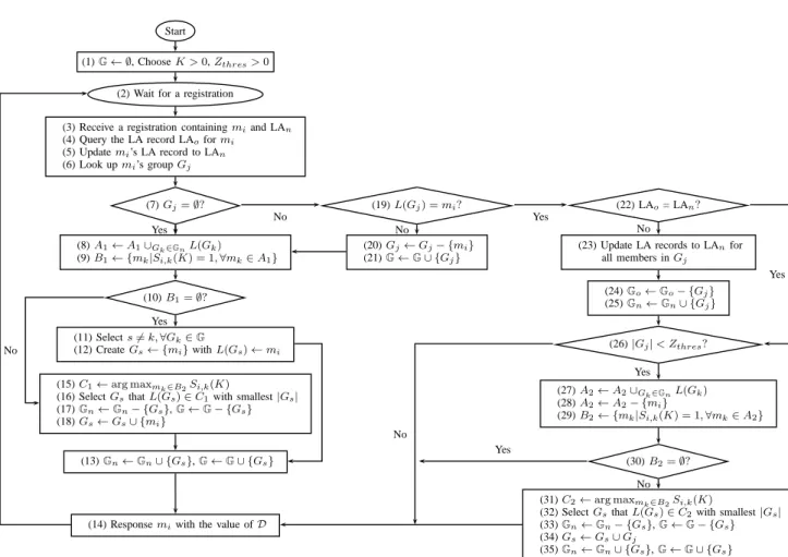
registration.

LDB part: In GLM, the LDB in the network is responsible for the group maintenance and location management for MSs, including determining the T

P LU

and

S values

for each MS. Figure 2.1 illustrates the flow chart for the LDB part. The notations are introduced as follows. The group i is denoted by the set G

_i

that contains an amount of MSs, and the group leader of G

_i

is denoted by L(G

_i

), where L(G

_i

)

∈ G i

. For

example, L(G

₁

) = m

₄

means that the leader of the group G

₁

is the MS m

₄

. LetG denote the group set that contains all groups in the network. Let the subsetG

i ⊆ G

denote the set containing the groups in LA

_i

,

∀i ∈ {1, 2, 3, ..., M}. It is clear that

G = G

1 ∪ G 2 ... ∪ G M

.

Initially, we set G ← ∅ and choose the values of K and Z

thres

(Steps 1 and 2), where K is the length of MS’ moving path maintained in the LDB, and Z

_thres

is the group size threshold to determine whether a group should be merged into another one. In GLM, a group can be merged with another group if the two groups of MSs have correlated mobility, and more registrations can be reduced. After the parameter initialization, the LDB waits to receive a location registration (Step 3).

When the LDB receives a location registration containing m

_i

and LA

_n

(where m

_i

is the MS identification and LA

_n

is the LAI to be registered), it queries the existing LA record for m

i

, denoted by LA

o

, and updates the LA record of m

i

to LA

n

. Then the LDB looks up the group information for m

i

(Steps 4 to 7). Suppose that m

i

belongs to the group G

_j

. We consider the following three cases.

Case I: G

j

=

∅. In this case, the LDB does not have any group records for the

MS m

i

, which implies that m

i

has just powered on and performs an initial registration. As shown in Steps 8 to 10, the LDB searches theG

n

set. Based on the search results, the LDB executes one of the following two operations:

Group creation: The LDB can not find any group inG

n

whose leader’s mov- ing path is similar to the m

_i

’s moving path (i.e., no group leader has cor- related mobility with m

_i

). The LDB creates a group G

_s

for m

_i

and sets

12

CHAPTER 2. GROUP-BASED MECHANISM FOR LOCATION MANAGEMENT L(G _s

)

← m i

(Steps 11 and 12).

Group assignment: The LDB finds a group G

_s

inG

n

whose leader’s moving path is similar to the m

_i

’s moving path. The LDB assigns m

_i

to the selected group G

_s

(Steps 15 to 18).

Case II: G

j ̸= ∅ and L(G j

)

̸= m i

. In this case, m

i

is a member of the group G

j

. The LDB removes m

_i

from G

_j

(Steps 20 and 21). Then the LDB searches the G

n

set and performs one of the two operations mentioned in Case I for m

_i

, i.e., group creation or assignment.

Case III: G

j ̸= ∅ and L(G j

) = m

i

. In this case, m

i

is the leader of the group

G _j

. As LA

o ̸= LA n

(i.e., the registration is triggered due to LA change), the LDB updates the LA records for the entire group members in G

_j

(Step 23), and updates the corresponding G

o

and G

n

sets (Steps 24 and 25). Then, the LDB checks whether the group size

|G j | is smaller than Z thres

to determine whether the group G

_j

should be merged (Step 26). If

|G j | < Z thres

, the LDB performs the following merge operation:

Group merge: The LDB searches theG

n

set to find a proper group to merge with (except its own group G

_j

). The selected group G

_s

satisfies two con- straints: the moving path of L(G

_s

) is similar to the moving path of m

_i

(Step 29), and the group size of G

s

is the smallest (Step 32). Then the merge is performed (Step 34). After group merge, m

i

is no longer the leader of G

_j

and becomes a member of G

_s

.

After each operation, the LDB updates the group G

_s

to theG

n

andG sets (Step 13).

Based on the status of m

_i

(i.e., leader or member), the LDB responses m

_i

with the value of

D through the acknowledgement message (Step 14).

2.3 Discussion

As mentioned in Chapter 1, to route an incoming session to an MS, the CN queries the LDB to obtain the LAI for the MS and instructs all cells in the LA to page the MS. If the MS does not reside in the LA, the CN can not receive the response from the MS in a given time period. Therefore, the CN can not locate the MS to route the incoming session. This phenomenon is called “page miss”.

With the GLM mechanism, we can reduce significantly the registration signaling over- head and mitigate the signaling congestion problem. However, the GLM mechanism may result in higher page miss probability. Consider four MSs m

1

, m

2

, ..., m

4

in the LA

1

, and the four MSs belong to the same group with the leader m

₁

. Assume that the leader m

₁

moves to LA

₂

at time t

₁

, the members m

₂

and m

₃

move together with m

₁

at t

₁

, and the member m

₄

moves to LA

₂

at t

₂

, where t

₁ < t ₂

. At t

₁

, a registration due to LA change is executed by m

₁

to update the LA record from LA

₁

to LA

₂

in the LDB. Therefore, at t

₁

, the LA records for m

1

, m

2

, ..., m

4

are updated to LA

2

. Yet the member m

4

still resides in LA

1

until t

2

. Therefore, during the time period [t

1 , t ₂

], the m

₄

’s LA record in the LDB is not correct, and the pages to the member m

₄

are missed. During [t

₁ , t ₂

], if m

₄

performs the periodic registration (i.e., on the expiration of the T

_{P LU}

timer), the m

₄

’s LA record in the LDB will be corrected, and the LDB will divide m

₄

from the group.

Chapter 3

Performance Evaluation

In this chapter, we develop simulation experiments to investigate the performance of the GLM mechanism. In Chapter 3.1, we define two performance metrics, the signaling reduction ratio

R and page miss ratio P. In Chapter 3.2, we propose three mobility

models for M2M communications to reflect different temporal and/or spatial correlations among MSs. In Chapter 3.3, we introduce our simulation models and parameter setups.

Finally, Chapter 3.4 presents the performance evaluation for the GLM mechanism.

3.1 Performance Metrics

Observing the N MSs for a given time period T , we evaluate the GLM mechanism based on the two performance metrics, the signaling reduction ratio

R and page miss ratio P,

with the following definitions.

Signaling reduction ratio

R: During the observation period T , let N r,GLM

denote the

14

number of the total registrations executed by the N MSs for the GLM mechanism.

Let N

_r

denote the number of the total registrations executed by the N MSs for the standard location management mechanism (as mentioned in Chapter 2), where

N r,GLM ≤ N r

. The signaling reduction ratio

R can be expressed as

R = E[N _r

]

− E[N r,GLM

]

E[N _r

]

,

where 0

≤ R ≤ 1. A larger R ratio implies larger reduction of registration signal-

ing overhead.

Page miss ratio

P: During T , let N p

denote the number of pages issued by the CN for the N MSs, and N

_p,miss

denote the number of page misses in N

_p

pages, where

N _p,miss ≤ N p

. The page miss ratio

P is defined as

P = E[N _p,miss

]

E[N _p

]

,

where 0

≤ P ≤ 1. A higher P ratio implies that the CN has higher possibility to

have a page miss, resulting in a higher risk of undeliverable incoming sessions.

3.2 Mobility Models

In this paper, we use three MS mobility models to reflect different levels of temporal and/or spatial correlation among the MSs. We consider the N MSs moving around in the

M LAs. Without loss of generality, we assume the mesh LA structure and M = w ²

. In the mesh LA structure, the size of an LA is square shaped. An LA is indexed by (x, y),

16

CHAPTER 3. PERFORMANCE EVALUATION

(1,1) (1,2) (1,3) (1,4) (2,1) (2,2) (2,3) (2,4) (3,1) (3,2) (3,3) (3,4) (4,1) (4,2) (4,3) (4,4)

Figure 3.1: The 4

× 4 mesh LA network structure

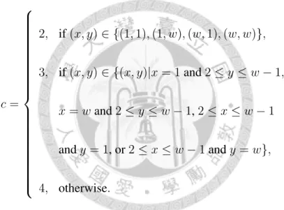
where x, y

∈ {1, 2, 3, ..., w}. The LA (x, y) has c neighboring LAs, where

c =











































2, if (x, y)

∈ {(1, 1), (1, w), (w, 1), (w, w)},

3, if (x, y)

∈ {(x, y)|x = 1 and 2 ≤ y ≤ w − 1,

x = w and 2 ≤ y ≤ w − 1, 2 ≤ x ≤ w − 1

and y = 1, or 2

≤ x ≤ w − 1 and y = w},

4, otherwise.

Figure 3.1 illustrates the mesh LA network structure with 16 LAs. In our mobility models, the size of LAs are indirectly reflected by the LA residence time. If the LA size is large, the mean LA residence time is relatively long, and vice versa.

Initially, the locations of the N MSs are uniformly distributed to M LAs. To sim- ulate different levels of correlation in terms of time and space, we consider three kinds of mobility models for M2M communications, including the random walk, bio-inspired mobility and transportation mobility models. The three mobility models are described as follows:

Random walk: An MS decides its own moving direction and LA residence time inde- pendently and randomly. Specifically, suppose that the MS resides in the LA (x, y) for a time period and the MS moves to one of (x, y)’s neighboring LAs with the equal probability. In this mobility model, there is no temporal and spatial correla- tion among MSs.

Bio-inspired mobility: This mobility model is designed based on the concept of the bird- flocking behavior [15], which is described as follows:

The MSs distributed to the same LA form a “cluster”

¹

, and then we have M clusters in the network. There is a cluster head in each cluster. Consider an arbitrary cluster that contains X MSs. In the beginning, the cluster head and the other X

− 1 MSs

are in the same LA, supposing they reside in (x, y) at time t. Each MS has its own LA residence time for (x, y). Assume that the cluster head resides in (x, y) for the period t

_ch

, and the other X

−1 MSs reside in (x, y) for the periods t 1 , t ₂ , t ₃ , ..., t _{X −1}

, respectively. At t + t

_ch

, the cluster head moves to one of (x, y)’s neighboring LAs with the equal probability. Consider one of the X

− 1 MSs leaving (x, y) at t + t _i

, where i = 1, 2, 3, ..., X

− 1. If t i < t _ch

(i.e., the MS leaves (x, y) earlier than the cluster head), the MS “disperses” its cluster and moves to one of (x, y)’s neighboring LAs with the equal probability. Otherwise (i.e., t

i > t _ch

), the MS

“follows” the moving direction of the cluster head.

1 Note that the term “cluster” is different from the term “group”. The term cluster is used to describe

the MS mobility behavior (i.e., the MSs in the same cluster have correlated mobility), and the term group is

used in the GLM mechanism for location management as mentioned in Chapter 2.

18

CHAPTER 3. PERFORMANCE EVALUATION

For the MS dispersed from its cluster (i.e., the MS moves to an LA different from the LA in which the cluster head resides), it moves toward the head’s residing LA (i.e., the MS “returns” to the cluster head’s LA), and the moving path is calculated by using the shortest path algorithm. Note that if there exist multiple shortest paths, we randomly choose one.

In this mobility model, the MSs have certain levels of temporal and spatial correla- tions.

Transportation mobility: This mobility model simulates the scenario where the MSs are in the same vehicle. Similar to the bio-inspired mobility model, the MSs distributed to the same LA form a cluster and we have M clusters in the network. In each cluster, there is a cluster head, and the cluster head decides the moving direction and LA residence time for the other MSs in the same cluster. The moving direction is decided randomly. In this mobility model, there exists very high correlation among MSs in terms of time and space.

3.3 Simulation Models

We develop the simulation experiments for the GLM mechanism based on the discrete event-driven approach. In the simulation experiments, we consider a 4

× 4 LA mesh

structure (i.e., M = 16 as shown in Figure 3.1). We observe the N = 640 MSs moving around in the 4

× 4 LA mesh structure for a time period T = 3000 minutes. We assume

that the page arrivals to an MS form the Possion process with rate λ

_p

, and the mean

inter-page arrival time 1/λ

_p

is set to 100 minutes. In our simulation experiments, the LA residence time t

_r

is exponentially distributed. The three proposed mobility models (as mentioned in Chapter 3.2) are implemented in this chapter.

We first define four types of events listed as follows:

• The CLUSTERCROSSBOUND event represents that a cluster crosses boundary

of LA. It is used only in transportation mobility model.

• The CROSSBOUND event represents that an MS crosses boundary of LA.

• The PAGING event represents that a paging arrival of an MS.

• The PLU event represents that an MS performs periodic location update, i.e., the

periodic location update timer of the MS is expired.

The following counters are used in our simulation to calculate the output measures

R and P :

• N LU

counts the total number of CROSSBOUND events.

• N LLU

counts the total number of CROSSBOUND events which performed by group leaders.

• N P

counts the total number of PAGING events.

• N P M

counts the total number of page miss.

• N P LU

counts the total number of PLU events.

20

CHAPTER 3. PERFORMANCE EVALUATION

We repeat the simulation runs until t

_s

exceeds the time period T , which is a predefined positive number, to ensure the stability of the simulation results. Two output measures are investigated in our models, including the signaling reduction ratio

R and the page miss

ratio

P (as mentioned in Chapter 3.1).

3.3.1 Random Walk Model

Figure 3.4 illustrates the flowchart of random walk mobility simulation model. Step 1 sets up the input parameters (including N, K, λ

_c , λ _p , Z _thres ,and T _{P LU}

). In addition, the counters (e.g., N

_LU , N _LLU , N _p , N _{P M} , and N _{P LU}

are set to zero, and the event queue is set to empty. Step 2 sets a initial GTable which has the functionality of GLM. Step 3 generates CROSSBOUND, PAGING, and PLU events for each MS. The timestamp of each event is set to zero. Step 4 removes the next event e from the event queue, and set the value of t

s

to e.timestamp. Step 5 checks the type of event e.

If event e is a CROSSBOUND event at Step 5, Step 6 increases N

_LU

by one. Step 7 randomly selects a nLA which is the neighbor LA of the current LA of the MS. Step 8 sets e.LA to nLA. Step 9 stores the nLA to the moving path of MS. Step 10 checks the state

D of MS. If MS.D equals to 1 that means the MS is a leader of group, the Step 11

increases the N

LLU

by one. Step 12 updates the moving path of the MS to GTable and execute the GLM. The progress of GLM has shown in Fig. 2.1. Step 13 checks the return value

D of GLM. If the D equals to 1, Step 14 sets the MS.D to 1. Otherwise, step 15 sets

the MS.

D to 0. Step 16 generates the next CROSSBOUND event of the MS and inserts

it to the event queue. This simulation goes to Step 17.

If event e is a PAGING event at Step 5, Step 18 increases N

_p

by one. Step 19 sets cLA to the current LA which the GTable stored of the MS. Step 20 checks whether the cLA equals to nLA. If not (e.g., paging miss), Step 21 increases N

_{P M}

by one. Step 22 generate the next PAGING event of the MS and inserts it to the event queue.This simulation goes back to Step 17.

If event e is a PLU event at Step 5, Step 23 increases N

_{P LU}

by one. Step 24 updates the moving path of the MS to GTable and executes the GLM. Step 25 checks whether the return value

D of GLM is equals to 1. If so, Step 26 sets MS.D to 1. Otherwise, Step 27

sets the MS.

D to 0. Step 28 generates the next PLU event of the MS and inserts it to the

event queue. This simulation goes back to Step 17.

If the timestamp t

_s

is less than 3,000 at Step 17, the simulation goes back to the Step 4. Otherwise, the simulation will be terminated and calculate the output measures

P and R at Steps 29 and 30.

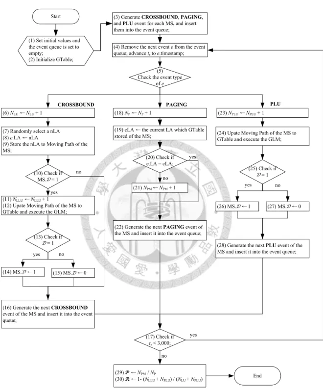
3.3.2 Bio-inspired Mobility Model

Figure 3.3 illustrates the flowchart of bio-inspired mobility simulation model. Step 1 sets up the input parameters (including N, K, λ

_c , λ _p , Z _thres ,and T _{P LU}

). In addition, the counters (e.g., N

LU , N LLU , N p , N P M , and N P LU

are set to zero, and the event queue is set to empty. Step 2 sets a initial GTable which has the functionality of GLM. Step 3 initializes N

_c

clusters and randomly distributes them into M network. Step 4 initializes

N MSs and randomly distributes them into N _c

clusters. Step 5 randomly selects a MS to be the head of cluster for each cluster. Step 6 generates CROSSBOUND, PAGING, and

22

CHAPTER 3. PERFORMANCE EVALUATION

(3) Generate CROSSBOUND, PAGING, and PLU event for each MS, and insert them into the event queue;

(4) Remove the next event e from the event queue; advance t

s

to e.timestamp;

CROSSBOUND PAGING PLU

Start

(5) Check the event type

of e

(6) N

LU

← N

LU

+ 1 (18) N

P

← N

P

+ 1 (23) N

PLU

← N

PLU

+ 1

(28) Generate the next PLU event of the MS and insert it into the event queue;

(25) Check if

= 1

(26) MS. ← 1 (27) MS. ← 0 (24) Upate Moving Path of the MS to GTable and execute the GLM;

yes no

(11) N

LLU

← N

LLU

+ 1

(12) Upate Moving Path of the MS to GTable and execute the GLM;

(7) Randomly select a nLA (8) e.LA ← nLA

(9) Store the nLA to Moving Path of the MS;

(13) Check if

= 1

(14) MS. ← 1 (15) MS. ← 0

yes no

(10) Check if MS. = 1

yes

(16) Generate the next CROSSBOUND event of the MS and insert it into the event queue;

(22) Generate the next PAGING event of the MS and insert it into the event queue;

(20) Check if e.LA = cLA;

(21) N

PM

← N

PM

+ 1 no

yes no

(17) Check if t

_s

< 3,000;

(29) च ← N

PM

/ N

P

End

(30) ज ← 1- (N

^LLU

+ N

PLU

) / (N

LU

+ N

PLU

) no

yes (1) Set initial values and

the event queue is set to empty;

(2) Initialize GTable;

(19) cLA ← the current LA which GTable stored of the MS;

Figure 3.2: Flowchart of random walk mobility simulation model.

PLUevents for each MS and inserts them into the event queue.The timestamp of each event is set to zero. Step 7 removes the next event e from the event queue, and set the value of t

_s

to e.timestamp. Step 8 checks the type of event e.

If event e is a CROSSBOUND event at Step 8, Step 9 increases N

LU

by one. Step 10 checks whether the MS is a head of cluster. If so, Step 11 randomly selects a nLA.

Otherwise, Step 12 selects a nLA which is near to head’s residing LA. Step 13 sets e.LA to the selected nLA. Step 14 stores the nLA to the moving path of the MS. Step 15 checks if the state

D of the MS is equals to 1. If so, Step 16 increases N LLU

by one. Step 17 updates the moving path of the MS to GTable and executes the GLM. The progress of GLM has shown in Fig. 2.1. Step 18 checks the return value

D of GLM is equals to 1. If

so, Step 19 the sets MS.

D to 1. Otherwise, Step 20 sets MS.D to 0. Step 21 generates the

next CROSSBOUND event of the MS and inserts it to the event queue. This simulation goes to Step 22.

If event e is a PAGING event at Step 8, Step 23 increases N

_p

by one. Step 24 sets cLA to the current LA which the GTable stored of the MS. Step 25 checks whether the cLA equals to nLA. If not (e.g., paging miss), Step 26 increases N

_{P M}

by one. Step 27 generate the next PAGING event of the MS and inserts it to the event queue. This simulation goes back to Step 22.

If event e is a PLU event at Step 8, Step 28 increases N

P LU

by one. Step 29 updates the moving path of the MS to GTable and executes the GLM. Step 30 checks whether the return value

D of GLM is equals to 1. If so, Step 31 sets MS.D to 1. Otherwise, Step 32

sets the MS.

D to 0. Step 33 generates the next PLU event of the MS and inserts it to the

24

CHAPTER 3. PERFORMANCE EVALUATION

event queue. This simulation goes back to Step 22.

If the timestamp t

_s

is less than 3,000 at Step 22, the simulation goes back to the Step 7. Otherwise, the simulation will be terminated and calculate the output measures

P and R at Steps 34 and 35.

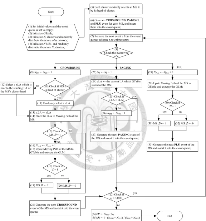
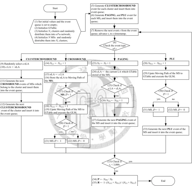
3.3.3 Transportation Mobility Model

Figure 3.2 illustrates the flowchart of bio-inspired mobility simulation model. Step 1 sets up the input parameters (including N, K, λ

c , λ _p , Z _thres ,and T _{P LU}

). In addition, the coun- ters (e.g., N

_LU , N _LLU , N _p , N _{P M} , and N _{P LU}

are set to zero, and the event queue is set to empty. Step 2 sets a initial GTable which has the functionality of GLM. Step 3 initializes

N _c

clusters and randomly distributes them into M network. Step 4 initializes N MSs and randomly distributes them into N

_c

clusters. Step 5 generates CLUSTERCROSS- BOUNDevents for each cluster and inserts them into the event queue. Step 6 generates CROSSBOUND, PAGING, and PLU events for each MS and inserts them into the event queue.The timestamp of each event is set to zero. Step 7 removes the next event e from the event queue, and set the value of t

_s

to e.timestamp. Step 8 checks the type of event e.

If event e is a CLUSTERCROSSBOUND event at Step 8, Step 9 randomly selects a nLA. Step 10 sets the e.LA to nLA. Step 11 generates the next CROSSBOUND events of the MSs which belong to this cluster and inserts them into event queue. The timestamp of the CROSSBOUND events is set to t

_s

. Step 12 generates the next CLUSTERCROSS- BOUNDevent of the cluster and inserts it into the event queue. This simulation goes to Step 13.

(10) Check if MS is a head of cluster

(11) Randomly select a nLA (12) Select a nLA which is

near to the residing LA of the MS’s cluster head.

(5) Each cluster randomly selects an MS to be its head of cluster.

(6) Generate CROSSBOUND, PAGING, and PLU event for each MS, and insert them into the event queue;

(7) Remove the next event e from the event queue; advance t

s

to e.timestamp;

CROSSBOUND PAGING PLU

Start

(8) Check the event type

of e

(9) N

LU

← N

LU

+ 1 (23) N

P

← N

P

+ 1 (28) N

PLU

← N

PLU

+ 1

(33) Generate the next PLU event of the MS and insert it into the event queue;

(30) Check if

= 1

(31) MS. ← 1 (32) MS. ← 0 (29) Upate Moving Path of the MS to GTable and execute the GLM;

yes no

(16) N

LLU

← N

LLU

+ 1

(17) Upate Moving Path of the MS to GTable and execute the GLM;

(13) e.LA ← nLA

(14) Store the nLA to Moving Path of the MS;

(18) Check if

= 1

(19) MS. ← 1 (20) MS. ← 0

yes no

(15) Check if MS. = 1

yes

(21) Generate the next CROSSBOUND event of the MS and insert it into the event queue;

(27) Generate the next PAGING event of the MS and insert it into the event queue;

(25) Check if e.LA = cLA;

(26) N

PM

← N

PM

+ 1 no

yes

no

(22) Check if t

_s

< 3,000;

(34) च ← N

^PM

/ N

P

End

(35) ज ← 1- (N

LLU

+ N

PLU

) / (N

LU

+ N

PLU

) no

yes (1) Set initial values and the event

queue is set to empty;

(2) Initialize GTable;

(3) Initialize N

c

clusters and randomly distribute them into ω*ω network;

(4) Initialize N MSs and randomly distriubte them into N

c

clusters;

(24) cLA ← the current LA which GTable stored of the MS;

no

yes

Figure 3.3: Flowchart of bio-inspired mobility simulation model.

26

CHAPTER 3. PERFORMANCE EVALUATION

If event e is a CROSSBOUND event at Step 8, Step 14 increase the N

_LU

by one. Step 15 sets nLA to e.LA. Step 16 stores teh nLA to the moving path of the MS. Step 17 checks if the MS.

D is equals to 1. If so, Step 18 increases the N LLU

by one. Step 19 updates the moving path of the MS to GTable and execute the GLM. The progress of GLM has shown in Fig. 2.1. Step 20 checks the return value

D of GLM. If the D equals to 1, Step 21 sets

the MS.

D to 1. Otherwise, step 22 sets the MS.D to 0. This simulation goes back to Step

13.

If event e is a PAGING event at Step 8, Step 23 increases N

p

by one. Step 24 sets cLA to the current LA which the GTable stored of the MS. Step 25 checks whether the cLA equals to nLA. If not (e.g., paging miss), Step 26 increases N

_{P M}

by one. Step 27 generate the next PAGING event of the MS and inserts it to the event queue. This simulation goes back to Step 13.

If event e is a PLU event at Step 8, Step 28 increases N

_{P LU}

by one. Step 29 updates the moving path of the MS to GTable and executes the GLM. Step 30 checks whether the return value

D of GLM is equals to 1. If so, Step 31 sets MS.D to 1. Otherwise, Step 32

sets the MS.

D to 0. Step 33 generates the next PLU event of the MS and inserts it to the

event queue. This simulation goes back to Step 13.

If the timestamp t

s

is less than 3,000 at Step 13, the simulation goes back to the Step 7. Otherwise, the simulation will be terminated and calculate the output measures

P and

R at Steps 34 and 35.

(11) Generate the next

CROSSBOUND events of MSs which belong to the cluster and insert them into the event queue;

CLUSTERCROSSBOUND

(12) Generate the next CLUSTERCROSSBOUND

event of the cluster and insert it into the event queue;

(9) Randomly select a nLA (10) e.LA ← nLA

(5) Generate CLUSTERCROSSBOUND event for each cluster and insert them into event queue;

(6) Generate PAGING, and PLU event for each MS, and insert them into the event queue;

(7) Remove the next event e from the event queue; advance t

s

to e.timestamp;

CROSSBOUND PAGING PLU

Start

(8) Check the event type

of e

(14) N

LU

← N

LU

+ 1 (23) N

P

← N

P

+ 1 (28) N

PLU

← N

PLU

+ 1

(33) Generate the next PLU event of the MS and insert it into the event queue;

(30) Check if

= 1

(31) MS. ← 1 (32) MS. ← 0 (29) Upate Moving Path of the MS to GTable and execute the GLM;

yes no

(18) N

LLU

← N

LLU

+ 1

(19) Upate Moving Path of the MS to GTable and execute the GLM;

(15) nLA ← e.LA

(16) Store the nLA to Moving Path of the MS;

(20) Check if

= 1

(21) MS. ← 1 (22) MS. ← 0

yes no

(17) Check if MS. = 1

yes

(27) Generate the next PAGING event of the MS and insert it into the event queue;

(25) Check if e.LA = cLA;

(26) N

PM

← N

PM

+ 1 no

yes

no

(13) Check if t

_s

< 3,000;

(34) च ← N

^PM

/ N

P

End

(35) ज ← 1- (N

LLU

+ N

PLU

) / (N

LU

+ N

PLU

) no

yes (1) Set initial values and the event

queue is set to empty;

(2) Initialize GTable;

(3) Initialize N

c

clusters and randomly distribute them into ω*ω network;

(4) Initialize N MSs and randomly distriubte them into N

c

clusters;

(24) cLA ← the current LA which GTable stored of the MS;

Figure 3.4: Flowchart of transportation mobility simulation model.

28

CHAPTER 3. PERFORMANCE EVALUATION

3.4 Simulation Results

In this Chapter, we investigate the performance of GLM by studying the effects of the parameters K, T

_{P LU}

and E[t

_r

] on

R and P. The details are given as follows.

3.4.1 Effects of K

In Figure 3.5, we investigate the effects of K (i.e., the length of the MS’ moving path maintained in the LDB) on

R and P, where we set Z thres

= 10, ϵ = 2 minutes, E[t

_r

] = 10 minutes, 1/λ

_p

= 100 minutes, and T

_{P LU}

= 60 minutes.

As shown in Figure 3.5(a), as K increases, it is less likely for the GLM mechanism to form groups for MSs, so less registration signaling overhead can be reduced. We observe that the

R performance decreases as K increases. On the other hand, in Figure 3.5(b), as K increases, the MSs with correlated mobility are more likely to be grouped by the GLM

mechanism. Thus, better

P performance is observe when K increases. It is also worth

to noticing that as K > 5, the GLM mechanism can not reduce the registration signaling (i.e., the

R performance is zero) for the random walk and bio-inspired mobility models.

In Figure 3.5, we also investigate the

R and P performance for the three mobility

models. The GLM mechanism has very good

R and P performance for the transportation

mobility model due to the high correlation among MSs. In Figure 3.5(a), as K > 5, we observe that

R for the bio-inspired mobility is higher than R for the random walk (i.e.,

more registration signaling can be saved in the bio-inspired mobility). On the other hand, in Figure 3.5(b), as K > 5,

P for the bio-inspired mobility is only higher than P for the

random walk slightly.

To summarize, when the temporal and spatial correlation among MSs becomes higher (i.e., the MSs have higher chance to have correlated mobility behaviors), the GLM mech- anism can reduce larger registration signaling overhead.

3.4.2 Effects of Periodic Location Update Timer T P LU

In Figure 3.6, we investigate the effects of T

_{P LU}

on

R and P, where we set Z thres

= 10,

ϵ = 2 minutes, K = 2, E[t _r

] = 10 minutes, and 1/λ

_p

= 100 minutes.

As mentioned in Chapter 2.1, the registration is triggered by LA change or T

P LU

expiration. In the GLM mechanism, the registrations due to the expiration of T

_{P LU}

can not be reduced. It turns out that as T

_{P LU}

increases, the number of the total registrations executed by an MS decreases, which magnifies the ratio for the reduced registrations due to LA change. Thus, we observe that the

R performance increases as T P LU

increases.

On the other hand, as mentioned in Chapter 2.3, the expiration of the T

P LU

timer can help GLM correct the wrong LA record in the LDB (that results in page miss). Therefore, in Figure 3.6(b), as T

_{P LU}

increases (i.e., it takes longer time for an MS to correct the wrong LA record), the

P performance increases (i.e., higher page miss probability).

To summarize, only when the MSs have correlated mobility (see the transportation mobility model in Figure 3.6) do we prefer to use a larger T

_{P LU}

timer. When the MSs do not have strong correlation between them (see the random walk or bio-inspired mobility models in Figure 3.6), to avoid high page miss probability, a small T

_{P LU}

is suggested.

30

CHAPTER 3. PERFORMANCE EVALUATION

3.4.3 Effects of LA Residence Time E[t r ]

In Figure 3.7, we investigate the effects of E[t

r

] (i.e., the mean LA residence time) on

R and P, where we set Z thres

= 10, ϵ = 2 minutes, K = 2, 1/λ

_p

= 100 minutes, and

T _{P LU}

= 60 minutes.

As shown in Figure 3.7(a), as E[t

r

] increases (i.e., an MS stays in an LA longer), the MS has less LA boundary crossings during T , so fewer registrations due to LA change can be reduced. Therefore, we observe that the

R performance decreases as E[t r

] increases.

On the other hand, in Figure 3.7(a), as E[t

_r

] increases, the

P performance decreases

because it is less likely that the LA record is not correct in the LDB.

3.4.4 Effects of Inter-Page Arrival Time 1/λ _p

In Figure 3.8, we investigate the effects of 1/λ

p

(i.e., the mean inter-page arrival time) on

R and P, where we set Z thres

= 10, ϵ = 2 minutes, K = 2, E[t

_r

] = 10 minutes, and

T _{P LU}

= 60 minutes.

In Figure 3.8(a) and Figure 3.8(b), we observe that both

R and P performance are

insensitive to the mean inter-page arrival time for the three kinds of mobility models.

1 2 3 4 5 6 7 8 9 10 K

0 10 20 30 40 50 60 70 80 90

R (%)

...

•

•

•

• • • • • • •

...

/ / / / / / / / / /

...

...

◦

◦

◦

◦ ◦ ◦ ◦ ◦ ◦ ◦

• Random walk

◦ Bio-inspired mobility

/ Transportation mobility

(a) Signaling reduction ratio

1 2 3 4 5 6 7 8 9 10 K

0 10 20 30 40 50 60 70 80

P (%)

...

...

...

•

•

•

• • • • • • •

...

...

/

/ / / / / / / / /

...

...

...

◦

◦

◦

◦ ◦ ◦ ◦ ◦ ◦ ◦

• Random walk

◦ Bio-inspired mobility

/ Transportation mobility

(b) Page miss ratio

Figure 3.5: Effects of K on

R and P for three mobility models, where Z thres

= 10,

ϵ = 2 minutes, E[t r

] = 10 minutes, 1/λ

p

= 100 minutes, T

P LU

= 60 minutes.

30 40 50 60

T _{P LU} (unit: minute) 0

10 20 30 40 50 60 70 80 90

R (%)

...

•

•

•

•

...

/

/

/ /

...

◦

◦

◦

◦

• Random walk

◦ Bio-inspired mobility

/ Transportation mobility

(a) Signaling reduction ratio

30 40 50 60

T _{P LU} (unit: minute) 0

10 20 30 40

P (%)

...

•

•

•

•

...

/ / / /

...

◦

◦

◦

◦

• Random walk

◦ Bio-inspired mobility

/ Transportation mobility

(b) Page miss ratio

Figure 3.6: Effects of T

_{P LU}

on

R and P for three mobility models, where Z thres

= 10,

ϵ = 2 minutes, K = 2, E[t _r

] = 10 minutes, 1/λ

_p

= 100 minutes.

32

CHAPTER 3. PERFORMANCE EVALUATION

10 20 30 40 50 60 E [t r ] (unit: minute) 0

10 20 30 40 50 60 70 80 90

R

(%)

...

...

•

•

• • • •

...

...

/ /

/ /

/

...

/

...

◦

◦

◦

◦ ◦ ◦

• Random walk

◦ Bio-inspired mobility

/ Transportation mobility

(a) Signaling reduction ratio

10 20 30 40 50 60 E [t r ] (unit: minute) 0

10 20 30 40

P (%)

...

...

•

•

• • • •

...

/ / / / / /

...

...

◦

◦

◦

◦ ◦ ◦

• Random walk

◦ Bio-inspired mobility

/ Transportation mobility

(b) Page miss ratio

Figure 3.7: Effects of E[t

_r

] on

R and P for three mobility models, where Z thres

= 10,

ϵ = 2 minutes, K = 2, 1/λ _p

= 100 minutes, T

_{P LU}

= 60 minutes.

25 50 100 200

1/λ p (unit: minute) 0

10 20 30 40 50 60 70 80 90

R

(%) •

...

• • •

...

/ / / /

...

◦ ◦ ◦ ◦

• Random walk

◦ Bio-inspired mobility

/ Transportation mobility

(a) Signaling reduction ratio

25 50 100 200

1/λ p (unit: minute) 0

10 20 30 40

P (%)

...

• • • •

...

/ / / /

...

◦ ◦ ◦ ◦

• Random walk

◦ Bio-inspired mobility

/ Transportation mobility

(b) Page miss ratio

Figure 3.8: Effects of 1/λ

_p

on

R and P for three mobility models, where Z thres

= 10,

ϵ = 2 minutes, K = 2, E[t r

] = 10 minutes, T

P LU

= 60 minutes.

Chapter 4

Conclusion

In this paper, for large-scale M2M environment, we studied the signaling congestion prob- lem caused by simultaneous registrations from the MSs with correlated mobility. To re- duce the registration signaling overhead, we proposed the Group Location Management (GLM) mechanism. Based on the temporal and spatial correlations among MSs at the LDB, GLM divides MSs into different groups for “per-group” location management. In each group, the registration aggregation is done by selecting an MS to be the group leader and to perform the registration on behalf of the other members in the group. In GLM, the group management is performed by the LDB in the CN without involving the MSs.

There is no extra energy consumption and protocol modification for the MSs. However, the GLM mechanism may cause higher page miss probability, resulting in higher risk of undeliverable incoming session. To study the signaling reduction and page miss ratios, we conducted simulation experiments and considered three kinds of mobility models for M2M communications, including random walk, bio-inspired mobility and transportation

33

34

CHAPTER 4. CONCLUSION

mobility. Our study shows that the GLM mechanism can significantly reduce the regis- tration signaling overhead for MSs with correlated mobility.