Process Variability-Aware Transient Fault Modeling and Analysis

Process Variability-Aware Transient Fault Modeling and Analysis

Natasa Miskov-Zivanov, Kai-Chiang Wu, Diana Marculescu

Carnegie Mellon University {nmiskov,kcwu,dianam}@ece.cmu.edu

* This research was supported in part by NSF Award CNS0720653 and by Carnegie Mellon University's Cylab.

Abstract – Due to reduction in device feature size and supply voltage, the sensitivity of digital systems to transient faults is increasing dramatically. As technology scales further, the increase in transistor integration capacity also leads to the increase in process and environmental variations. Despite these difficulties, it is expected that systems remain reliable while delivering the required performance.

Reliability and variability are emerging as new design challenges, thus pointing to the importance of modeling and analysis of transient faults and variation sources for the purpose of guiding the design process. This work presents a symbolic approach to modeling the effect of transient faults in digital circuits in the presence of variability due to process manufacturing. The results show that using a nominal case and not including variability effects, can underestimate the SER by 5% for the 50% yield point and by 10% for the 90% yield point.

1.

The scaling of device feature sizes, operating voltages and design margins raises a great concern about the susceptibility of circuits to transient faults [3], [4], [7], [12], which can be caused by different physical phenomena, such as energetic particle hits originating from cosmic rays, capacitive coupling, electromagnetic interference, or power transients. Transient faults induced by radiation, also called Single-Event Transients (SETs), are claimed to be a major challenge for future scaling [4] and have thus been examined by many researchers in recent years. An error that results from an SET (glitch or pulse) is most often referred to as soft error or a single-event upset (SEU). The effect of soft errors is measured by the soft error rate (SER) in FITs (failure-in-time), which is defined as one failure in 10⁹ hours.

With the reduction of device dimensions and operating voltage, the impact of radiation in logic circuits is increasing and fast reaching the soft error rates in memories [17]. Hence, the importance of realistic and accurate projection of the SET-induced SER in logic (combinational and sequential) circuits is crucial in identifying the features needed for future reliable high-performance microprocessors.

As technology scales further, variations become prominent as well. Technology nodes beyond 90nm experience increasingly high levels of device parameter variations, which are changing the design flows from deterministic to probabilistic [3]. In general, there are three different sources of variation: environmental (supply voltage and operating temperature variation) and manufacturing (process variation). Process variations are expected to worsen in future technology generations due to difficulties with using standard lithography.

The performance of the chip is heavily dependent on the manufacturing process variations. When considering transient faults and their impact on circuit reliability, it is important to take into account the fact that the delay of a particular gate is no longer fixed across dies or within the same die, but instead should be characterized by a probability distribution. Furthermore, the propagation of a transient fault is a function of gate delay. In other words, variations in gate delays, resulting from process variations, can affect the size of the glitch propagated through the circuit and the circuit error rate [15].

To allow for the efficient design of a system that can tolerate faults, a first natural step includes understanding the source of induced errors, but most importantly, their modeling and analysis for the purpose of guiding the design process. The main goal of this work is to allow for accurate modeling and efficient estimation of the susceptibility of logic circuits to transient faults in the presence of variations of the process parameters. More specifically, we model the impact of variations in oxide thickness, Tox, number of dopants, Nch. gate length, Lg, and gate width, Wg, while also considering the spatial correlations that can exist between L_g or W_g for different gates. The rest of parameter variations are assumed to be independent.

The remainder of this paper is organized as follows. In Section 2, we describe previous work on transient fault and variation effect modeling and analysis and briefly outline the contributions of our work. Section 3 provides a motivating example for modeling variation effects in case of transient faults and the assumptions of the variation impact model. The proposed analytical model for glitch propagation when process variation impact is included is described in Section 4. An overview of our framework with the details about its implementation and the overall output error computation approach are presented in Section 5. Finally, in Section 6 we show the experimental results obtained using the proposed framework and with Section 7 we conclude our work.

2.

Among all transient faults, radiation-induced faults have received most of the attention in recent years, since they are considered as one of the major barriers for future technology scaling [4]. Intensive research has been done so far in the area of modeling, analysis, and protection for radiation-induced transient faults [7], [10]-[12], [16], [17]. Since our focus is on modeling of transient faults in the presence of process variations and the analysis of their effect on logic circuits, we give a brief overview of the work related to those aspects of transient faults in the sequel.

2.1. Transient fault modeling and analysis

A number of methods have been proposed recently to evaluate the susceptibility of logic circuits to soft errors, among them several symbolic models [10],[11]. An example of such symbolic modeling approach is the one that uses Binary Decision Diagrams (BDDs) and Algebraic Decision Diagrams (ADDs) to model the propagation of transient faults in logic circuits [10]. This model has been shown to be both efficient and accurate, and thus we incorporate its main ideas into our work.

2.2. Impact of process variations

Design variations or uncertainty in static timing analysis is typically handled in two ways. Traditional static timing methodology is corner based, e.g., best case, worst case, and nominal. Unfortunately, such a methodology may require an exponential number of timing runs as the number of independent and significant sources of variation increases. Furthermore, the analysis may be both pessimistic and risky at the same time [18].

Methods for statistical timing analysis were developed in recent years as a solution to these problems [6], [18], [19]. The central idea in statistical timing analysis is to capture the variability by modeling delays as distributions and performing timing analysis statistically by using these distributions. These timing analysis models most often assumed that process variations have a Gaussian probability distribution and that delay can be modeled using linear regression, thus resulting in a Gaussian probability distribution for delay as well.

2.3. Paper contribution

With respect to modeling transients faults, the main contribution of this work, when compared to previous work, is in allowing for accurate and efficient modeling and analysis of the impact of transient faults in logic (combinational and sequential) circuits when process variation effects are accounted for. To the best of our knowledge, there has only been one work that analyzed the impact of variations on SER [15], and there are several important differences between the approach described in [15] and our approach. In [15], custom designed circuits were simulated using HSPICE. The benchmark circuits considered by the authors were analyzed by running separate simulations for each discrete parameter value. Furthermore, the method in [15] assumes radiation-induced transient faults only. The contributions of our proposed framework, when compared to previous work, are included below:

• Our approach accurately models gate delay and glitch propagation by including simultaneous variation of several process parameters.

• Transient fault propagation is modeled using a non-simulative, symbolic approach that is orders of magnitude faster than HSPICE simulation.

• Gate delay and output glitch duration and amplitude are modeled explicitly as functions of process parameters.

• Our framework can be applied to any type of transient faults, not just radiation-induced faults.

As already stated in Sections 1 and 2.1, among all transient faults, radiation induced faults are predicted to be one of the main concerns in future chips [4]. Therefore, some of the aspects of our transient-fault modeling framework will be described in the sequel by focusing on single-event (radiation-induced) transients.

However, since specific parameters related to radiation induced transients (e.g., particle hit rate, ratio of effective hits) are not directly incorporated into the framework, but instead are included as inputs after all probabilities are computed, the proposed model is not restricted to radiation induced transient faults.

3.

When considering transient faults and their impact on circuit reliability, it is important to take into account the fact that the size of the propagated transient fault is a function of gate delay, which, in turn, is a function of process parameter variations. Thus, this section shows the results obtained from HSPICE simulations that further motivate the modeling and analysis of process variation- aware transient fault propagation. We also describe the assumptions necessary to create an efficient model and the pre-characterization method for our proposed model.

3.1. Motivating example

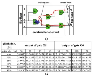
To provide a better understanding of the impact of process variations and, consequently, gate delay variations on the propagation of glitches through the circuit, we conducted several HSPICE simulations on benchmark circuit C17. We show in Figure

1 benchmark circuit C17, a glitch occurrence at the gate G₂ and two paths to gates G5 and G6. Assuming glitch occurrence at gate G2, we find the difference in the output glitch duration at the outputs of gates G5 and G6, for nominal case (nom.) and the case when process-driven parameter variations are included (yield points 10%, 20%, 50%, 75% and 90%). As it can be seen from Figure 1, there is a variation in output glitch duration, resulting from variations in process parameters and consequently gate delay. As it can be seen, while the nominal case output SET duration is not very far from the median case (50% y.p.), it can underestimate the output SET duration by more than 10% when compared to the 90% y.p., thus underscoring the importance of considering process variations in transient fault analysis. For larger circuits with larger number of gates and different gate types or for smaller technology nodes, more variations are expected to be seen in output glitch duration, and thus in final error rate as well.

3.2. Assumptions

There are several issues one needs to consider when modeling variation impact on glitch propagation through logic circuit. These issues lead to important assumptions about the model, as described next.

Variation sources distributions. Previous statistical timing analysis approaches have assumed Gaussian variation sources with good results. Thus, we approximate gate delay by a linear function of process parameters, each assumed to follow a Gaussian distribution.

Also, in our model, we consider correlations between parameters characterizing different gates.

Gate delay distribution. The simplest model for the gate delay under variability effects would be a Gaussian probability distribution. Reconvergent glitches may have correlated duration and amplitude distributions due to propagation through gates with correlated parameters. To take these correlations into account, it is necessary to represent gate delay as a function of the varying process parameters. We consider that all gate delays can be represented as a linear combination of the variations in oxide thickness, Tox, number of dopants, Nch. gate length, Lg, and gate width, Wg.¹

Initial glitch duration and amplitude distribution. In previous work, initial glitch duration and amplitude, dinit and ainit have been assumed constant. However, including process variability

1 In the sequel, bold fonts designate random variables, while italics describe constant values.

a)

b)

Figure 1. Variation impact on transient fault propagation: a) circuit C17 and b) output glitch duration for nominal (nom.) case and with variations (10%, 20%, 50%, 75% and 90% yield point).

information significantly changes the problem. Since the glitch duration and amplitude are not independent, we assume that dinit

and ainit also follow a joint Gaussian distribution.

4.

The discussion in Section 3.2 highlighted several possible approaches to modeling variability-aware glitch propagation. This section provides the analytical treatment of transient fault propagation under Gaussian propagation delay distribution assumption, tprop: N(μ,σ²).

4.1. Transient fault propagation model

A linear model for the random variables representing the output glitch duration (dout) and amplitude (aout), as functions of propagation delay (tprop) and input glitch duration (din) and amplitude (ain) can be expressed as:

dout= c_d^t⋅ t_prop+ c_d^d⋅ d_in+ c_d^a⋅ a_in+ c_d (1) a_out= c_a^t⋅ t_prop+ c_a^d⋅ d_in+ c_a^a⋅ a_in+ c_a (2) or, in matrix representation:

B HX

Y= + (3)

where X=

t_prop d_in ain

⎡

⎣

⎢ ⎢

⎢

⎤

⎦

⎥ ⎥

⎥ , _Y= ^dout

a_out

⎡

⎣ ⎢ ⎤

⎦ ⎥ ,_H= ^cd t c_d^d c_d^a c_a^t c_a^d c_a^a

⎡

⎣ ⎢ ⎤

⎦ ⎥ , _B=^cd c_a

⎡

⎣ ⎢ ⎤

⎦⎥.

Assuming that X is a Gaussian random vector with mean vector MX

and covariance matrix Σ_X and using the properties of a characteristic function of random variable, we can compute the mean MY and covariance matrix ΣY of Y as [9]:

MY= HM_X+ B (4)

Σ_Y= HΣ_XH^T (5)

4.2. Process parameter variation-aware model

We have assumed in previous discussion that the gate delay is a random variable with Gaussian distribution. However, as already mentioned in Section 3.2, to accurately model transient fault propagation in the presence of variations, it is necessary to account for gate delay correlations. Therefore, we define gate delay as a linear function of variations in process parameters:

t_prop= t_prop0+ c_t^LΔL_g+ c_t^WΔW_g+ c_t^TΔT_ox+ c_t^NΔN_ch (6)

This also allows for expressing transient fault duration and amplitude in terms of process parameter variations:

d= d₀+ c_d^LΔL_g+ c_d^WΔW_g+ c_d^TΔT_ox+ c_d^NΔN_ch (7) a= a₀+ c_a^LΔL_g+ c_a^WΔW_g+ c_a^TΔT_ox+ c_a^NΔN_ch (8) leading to the following expression for computing d_out and a_out:

Y= HX+ B = H(AP + C) + B (9)

where A=

c_t^L c_t^W c_t^T c_t^N cdL cdL cdL cdL

c_a^L c_a^L c_a^L c_a^L

⎡

⎣

⎢ ⎢

⎢

⎤

⎦

⎥⎥

⎥ ,

P= ΔL_g ΔW_g ΔT_ox ΔN_ch

⎡

⎣

⎢ ⎢

⎢ ⎢

⎤

⎦

⎥ ⎥

⎥ ⎥ , _C= ^din,0

a_in,0

⎡

⎣ ⎢ ⎤

⎦ ⎥ .

Since we assume that Lg or Wg are correlated, a possible approach to model intra-die spatial correlations is to use the approach presented in [1]. The main idea is to divide the circuit into a number of regions using a multi-level quad-tree partition. For each level n, the die area is partitioned into 2²ⁿ× 2²ⁿ rectangles. The 0^th level contains one rectangle only that covers the entire chip. An independent random variable _L^{i, j}_g (_Wg^{i, j}) is assigned to each region (i, j) to model a portion of the total intra-die variations. The overall variation of parameter Lg (Wg) of a gate Gk is expressed as the sum of the individual components _L

g,n

i, j (_Wg,n^{i, j}) over all levels of the

regions that overlap with the location of the gate Gk. This approach allows for modeling spatial correlations in terms of independent random variables and for applying the approach described next for handling reconvergent glitches.

4.3. Reconvergent glitches

In the case of reconvergent glitches, that is, glitches originating as a single glitch but propagating to the inputs of the same gate on different paths, additional aspects of the modeling need to be considered. To find the output glitch(es) for the gate where reconvergent glitches arrive, it is necessary to merge these glitches according to their arrival time, size and logic values. The safest assumption for the variation-aware analysis is the worst-case one. In other words, in such situations, we analyze the chain of glitches as if they were merged into one large glitch.

As in the case of statistical timing analysis [18], two functions of Gaussian random variables need to be computed: sum and max.

When only one glitch at a time arrives at the gate, we only need to add the gate delay to the arrival time of the glitch. When two (or more) glitches arrive at the gate inputs, in order to merge them, we need to find the minimum of their arrival times, and maximum of the sum of their arrival times and durations. As described in previous work [6], [18], the computation of the sum function is straightforward, while finding the max among two or more Gaussian random variables is more complex. We apply the approach that uses the concept of tightness probability to find the minimum or maximum of two Gaussian random variables [18].

As shown in [18], given any two random variables a and b, the tightness probability T_a of a is the probability that a is larger than (or dominates) b. The tightness probability of b, Tb, is (1-Ta). Thus, using the tightness probability T, we can find the maximum of two random variables a and b as follows. First, we assume that, in general, variables a and b can be approximated linearly using a first-order Taylor expansion:

a= a₀+ aiΔp_i

i=1

∑

∑

where a0 and b0 are the mean (or nominal) values for variables a and b, respectively, Δpi, i=1,…,n represent the variation of n variation sources from their nominal values, and ai and bi, i=1,…,n give the sensitivities of variables a and b to each of the sources of variation. The first-order Taylor expansion is an acceptable approximation with little loss of accuracy when Δp_i is relatively small. This is generally true for typical process parameter variations values [5]. By using the hierarchical approach for modeling intra- die spatial correlations (Section 4.2), we can overcome the issue that arises due to parameter correlations and the independence of parameters pi assumed by the model described here.

The covariance matrix of variables a and b can be written as:

Cov(a,b)= ai2 i=1

∑

∑

a_ib_i

i=1

∑

∑

⎡

⎣

⎢ ⎢

⎢ ⎢

⎤

⎦

⎥ ⎥

⎥ ⎥

= σ_a² ρσ_aσ_b ρσ_aσ_b σ_b²

⎡

⎣ ⎢ ⎤

⎦ ⎥ (10)

where σa and σbare the standard deviations for variables a and b and ρ is their correlation coefficient.

Next, to find max(a,b), one can rely on the probability that a is larger than b [18]:

Ta= 1 σ_aφ ^{x− a0}

σ_a

⎛

⎝ ⎜ ⎞

⎠ ⎟ Φ x− b₀

σ_b

⎛

⎝ ⎜ ⎞

⎠ ⎟ −ρ ^{x− a0} σ_a

⎛

⎝ ⎜ ⎞

⎠ ⎟ 1−ρ²

⎛

⎝

⎜ ⎜

⎜ ⎜

⎞

⎠

⎟ ⎟

⎟ ⎟ dx

−∞

∞

∫

where φ and Φ are the standard normal probability density and cumulative distribution functions, respectively, and θ is defined as:

θ≡

(

)

The mean and variance of c = max(a,b) can now be analytically computed [18]:

μ_{max(a,b )}= c₀= a₀Ta+ b₀(1− T_a)+θφ ^{a0− b0} θ

⎛

⎝ ⎜ ⎞

⎠ ⎟ (13)

Var_max(a,B)=σ_C²=

(

)

(

)

+(a₀+ b₀)θφ ^{a0− b0} θ

⎛

⎝ ⎜ ⎞

⎠ ⎟ −μmax(a,b )2

(14)

We note that the max operation on two Gaussian random variables is not strictly Gaussian. However, as previously stated [5], for many applications this approximation is quite satisfactory. The coefficients c_i that correspond to parameters p_i in the expression for the variable c resulting from max(a,b) operation can be found as:

ci= Cov(c,p_i) (15)

and the correlation between c and pi can be computed as [5]:

ρc,p_i= σ_a⋅ρ_a,p

i⋅ Φ a₀− b₀

θ

⎛

⎝ ⎜ ⎞

⎠ ⎟ +σ_b⋅ρ_b,p

i⋅ Φ b₀− a₀

θ

⎛

⎝ ⎜ ⎞

⎠ ⎟

σ_c (16)

where ρ_a,p

i( ρ_b,p

i) are the correlation coefficients between variable a(b) and pi.

5.

In this section, we describe how the proposed analytical model from Section 4 was incorporated into an existing probabilistic symbolic framework [11], and how they can be used to evaluate the susceptibility of a logic circuit to transient faults.

The main aspects of the transient fault generation and propagation modeling methodology are shown in the block diagram in Figure 2. We first use HSPICE for pre-characterizing the impact of process parameter variations on gate delay and glitch size, as will be described in Section 5.1. Section 5.2 describes the preliminaries of transient fault analysis and the symbolic modeling approach on which our framework relies. In the final step of our approach, we describe the error probability computation.

5.1. Model pre-characterization

In order to obtain the parameters necessary for modeling glitch propagation through the circuit, we conducted the following experiments. For each gate type (inverter, NAND, NOR, XOR and XNOR), HSPICE simulations were run on a chain of gates of that type. A voltage source was connected to the input of the first gate in the chain to generate transient fault. Two sets of data were obtained, one for gate delay and one for the size of propagated glitch:

1. Delay variations. Gate delay was varied by changing the gate length, gate width, oxide thickness and number of dopants in the channel. All parameters are assumed to follow a Gaussian distribution, samples are generated randomly from parameter distributions and simulations are run for 1,000 parameter set samples. The standard deviation, σ, of different parameters is chosen as follows [5],[13]: 15% for gate length, Lg, 10% for gate

width, Wg, 5% for oxide thickness, Tox, and 5% for number of dopants, Nch. Response surface modeling (RSM) methodology [13]

is used to find a linear approximation for gate propagation delay as a function of this set of parameters, as in (6).

2. Glitch variations. Input glitch duration was varied in the interval [30,150]ps. Input amplitude is always assumed to be full swing (1V). Parameters with the aforementioned distribution and standard deviation are sampled 1,000 times. Due to gate delay variations, the glitch with a given initial size (i.e., duration and amplitude) produces different output glitch duration and amplitude values for the 1,000 samples after passing through the first gate.

Thus, these different duration and amplitude values are used to measure the impact of input duration and amplitude variations on the output glitch size at the second gate. The same measurements are obtained for other gates in the chain as well. The results obtained show the error of linear RSM method for output glitch duration. The approximation error in duration is most of the time very small with an average of a little over 4%, being on average less than 1% and 4% for NAND, NOR, and XNOR, with larger errors for the INV (inverter), and XOR gate (8% and 10%, respectively).

The results obtained by Monte Carlo HSPICE simulations are used in Matlab to compute the linear response surface models for gate delay and glitch duration and amplitude. Finally, the coefficients for approximation functions obtained from RSM are used by our symbolic modeling framework, together with the information about the circuit and the transient fault source parameters, as it can be seen from Figure 2.

5.2. Transient fault modeling

When a transient fault propagates through the circuits, there are three important masking factors that affect its propagation [10]:

logical masking (due to the other inputs with a controlling value), electrical masking (attenuation of the duration and amplitude of smaller glitches) and latching-window masking (due to setup and hold time conditions).

A practical implementation for SET modeling was described in [10], where a topologically sorted list of gates for a given circuit is generated first, and then, in one pass through the circuit, all possible glitches that can occur in the circuit are created and propagated to the primary outputs. The main idea of the approach proposed in [10]

is that the impact of the three masking factors can be modeled using BDDs and ADDs. When duration and amplitude ADDs representing a glitch originating at a given gate Gi are created, they are further propagated to the fanout neighbors of gate Gi, and there they are modified according to logical masking, the delay of those gates, and the attenuation model.

The important advantage of the proposed model is that it concurrently computes the propagation and the impact of single- event transients originating at different internal gates of the circuit and thus allows for efficient computation of circuit error susceptibility.

When propagating transient fault, we use the coefficients of d and a from the transient fault description in (1) and (2), and the gate delay coefficients (6) and apply equation (9) to find the output glitch duration and amplitude in terms of process parameter variations. In case of reconvergent glitches, as shown in the pseudocode in Figure 3, we first apply glitch merging, if necessary, as described in Section 4.3. After merging, we propagate the resulting glitch. Final glitch duration and amplitude ADDs are computed for all possible gate-output combinations, where gate represents the gate where glitch originated and output is the output at which the glitch arrived, as described in [10]. These final ADDs can be used to find the average probability of error at a given output for a given input vector probability distribution, as well as the Figure 2. Block diagram of the proposed approach.

impact of individual gates on outputs of the circuit, or on error susceptibility of the overall circuit [10].

5.3. Error probability computation

In this work, we model a transient fault’s duration and amplitude as a linear function of a set of random variables, as described in Section 4. We further find the probability of output Fj failing due to the propagation of the glitch from a given gate Gi, for a given initial glitch duration and amplitude and a given input vector probability distribution as [10]:

prob(F_jfails | G_ifails∩ (d_init,a_init))= d_k− (t_setup+ t_hold)

Tclk− d_init ⋅ k

∑ prob(d= d_k)

(17)

In other words, we find the sum over all possible glitch durations, dk, that occur at a given output and result from glitches originating at gate Gi. Tclk is the clock period, tsetup and thold are the setup and hold time of the latch, respectively, and dinit is the initial duration of the glitch that has duration d_k at the output. The initial glitch duration, dinit, is assumed to have a jointly normal distribution with initial amplitude, ainit, and the final glitch duration, dk, is a Gaussian random variable, dk. Since dinit is a Gaussian random variable, the probability computation in (17) includes a random variable in both parts of the fraction. This can be simplified by approximating the fraction with its Taylor expansion:

) ) (

(

) (

) 1 (

) (

) (

2 , ,

, ,

mean init init mean init clk

hold setup mean

mean mean init clk mean init clk

hold setup mean init

clk hold setup

d d T

t t d

d d T d

T

t t d T

t t

− − + + −

− −

− + +

≈ −

− +

−

d d d

d

(18)

We can now compute the Mean Error Susceptibility (MES), as suggested in [10], of a given output Fj, for given initial glitch duration and amplitude, dinit and ainit, as the average probability of output Fj failing due to all possible glitches that can occur in the circuit, given different input probability distributions:

MES(F_j^dinit,ainit)=

prob(Fjfails | Gifails∩ (d_init,ainit))

i=1 nG

∑

k=1 nf

∑

nG⋅ n_f (19)

where nG is the cardinality of the set of gates in the circuit {Gi} and nf is the cardinality of the set of probability distributions {fk}, associated to the input vector stream. Finally, we can find the overall probability of output Fj failing due to glitches at internal nodes as:

prob(Fj)= 1

n_l⋅ n_m MES(Fjdl,am)

m=1 n_m

∑

l=1 n_l

∑

Assuming, without loss of generality, that the surface of all allowed pairs for initial glitch duration and amplitude is partitioned into a grid, as shown in [10], it can be assumed that MES is the same within each sub-surface. Therefore, we average MES across all

allowed duration and amplitude values to find the probability of output Fj failing.

It can be concluded from equations (19) and (20) that all operations applied on random variables dk include only an addition or a multiplication by a constant, and thus, we can estimate the mean and provide bounds for the probability of error at circuit outputs, by applying the rules from probability theory [14].

Finally, having computed all the probabilities Fj, (that is, the mean and variance of P(Fj)) as in equation (20) for all outputs, we can use specific fault occurrence rate parameters to compute the final error rate. For example, in case of soft errors, resulting from radiation-induced transient faults, the soft error rate (SER) can be found as:

SER_Fj= prob(F_j)⋅ R_eff⋅ R_PH⋅ A_circuit (21)

where RPH is the particle hit rate per unit of area, Reff is the fraction of particle hits that result in charge generation, and Acircuit is the total silicon area of the circuit. Note that, since SER represents the number of failures that would occur every thousand hours per million devices, it can be translated into another reliability measure, Mean Time Between Failures (MTBF), which represents the overall time in all considered devices per number of failures. In Figure 3, we show the pseudocode of our main algorithm for computing circuit error susceptibility to transient faults.

6.

In this section, we first compare the results obtained using HSPICE simulator with the results obtained using our framework on a small example circuit C17. Then, we show the results of our symbolic modeling methodology for seven benchmark circuits, given different initial glitch durations and different sets of input probabilities. The technology used is 70nm, Berkeley Predictive Technology Model [20]. The clock cycle period (Tclk) used is 250ps, and setup (tsetup) and hold (thold) times for the latches are assumed to be 10ps each. Vdd is assumed to be 1V. The benchmark circuits are chosen from ISCAS’85 and mcnc’91 suite. The framework is implemented in C++ and run on a 3GHz Pentium 4 workstation running Linux.

In Table 1 the comparison between our proposed approach and HSPICE simulations is shown for circuit C17. HSPICE simulations are run for each circuit input combinations, considering each gate as a glitch source, and for four different initial glitch durations (30ps,

Figure 3. The main algorithm.

Table 1.

Relative error and speedup in estimating output glitch duration when compared to 1,000 Monte Carlo HSPICE simulation runs, for parameter variations as defined in Section 3.1, assuming different yield points (10%, 25%, 50% 75%, 90%) for circuit C17 and four different initial glitch durations (30ps, 70ps, 110ps and 150ps).

70ps, 110ps and 150ps), using 1,000 Monte Carlo approach runs for estimating the impact of parameter variations on glitch duration at the outputs of the circuit. As it can be seen from the figure, the error varies from 1% to 11% (5% on average), being largest for the shortest glitch durations. This error stems from the linear approximations of gate delay and glitch duration and amplitude, and from the worst-case assumption used in some cases of reconvergent glitch merging. However, the speedup, compared to HSPICE simulations with the Monte Carlo method is more than six orders of magnitude, up to 8×10⁶.

In Table 2, we show the SER for several benchmark circuits computed using equations (17-21) averaged across four different initial glitch durations (30ps, 70ps, 110ps and 150ps) and ten different random input vector probability distributions. The RPH

used is 56.5 m^-2s^-1, R_eff is 2.2·10^-5, and the total silicon area found for each benchmark circuit is proportional to the number of gates.

The SER is reported for the nominal case when all process parameters have fixed values, and for the 10%, 25%, 50%, 75%, and 90% yield point when variations of parameters are taken into account. It can be seen from the figure that using the nominal case, could underestimate the SER up to 5%, when compared to 50%

yield point and by 10% compared to 90% yield point. This translates into an overestimation of MTBF by 10% for 90% yield point (e.g., in today’s systems with hundreds of processors with millions of gates, instead of estimated 100 days for nominal case, the MTBF becomes 90 days in the presence of process variations).

The SER standard deviation σ varies for different circuits, due to different number of gates, the circuit topology and different gate types, having different variations in gate delay due to process variations.

7.

This work proposes a methodology for modeling transient fault propagation in the presence of process parameter variations. The main idea behind the proposed work is to allow for the efficient and accurate variability-aware analysis of the susceptibility of individual outputs to errors stemming from single transient faults.

We have demonstrated the efficiency of our method by applying it on a subset of ISCAS’85 and mcnc’91 benchmarks of various complexities and proved its accuracy by comparison with Monte Carlo simulations. Future work, will target using the framework to show the impact of technology scaling (65nm, 45nm) on SER in the presence of variations. Another important aspect of variation modeling is to model gate delay as a higher (e.g., second) order function of process parameter variations, as well as model some

parameter variations using distributions other than Gaussian (e.g., uniform distribution).

8.

[1] A. Agarwal, D. Blaauw, and V. Zolotov, “Statistical timing analysis for intra-die process variations with spatial correlations,” in IEEE International Conference on Computer Aided Design (ICCAD), pp. 900–907, 2003.

[2] K. Agarwal and S. Nassif, “Characterizing Process Variation in Nanometer CMOS,” in Proc. of Design Automation Conference (DAC), pp.

396-399, June 2007.

[3] S. Borkar, “Tackling variability and Reliability Challenges,” in IEEE Design and Test of Computers, Vol. 23, No. 6, pp. 520, June 2006.

[4] S. Borkar, “Thousand Core Chips – A Technology Perspective,” in Proc.

of Design Automation Conference (DAC), pp. 746-749, June 2007.

[5] H. Chang and S. S. Sapatnekar, “Statistical Timing Analysis Under Spatial Correlations,” in IEEE Transactions on Computer-Aided Design of Integrated Circuits and Systems (TCAD), Vol. 24, No. 9, pp. 1467-1482, September 2005.

[6] A. Devgan and C. Kashyap, “Block-based Static Timing Analysis with Uncertainty,” in Proc. of the IEEE/ACM International Conference on Computer-Aided Design (ICCAD), pp. 607-614, November 2003.

[7] P. E. Dodd, “Physics-Based Simulation of Single-Event Effects,” in IEEE Transactions on Device and Materials Reliability, Vol. 5, No. 3, pp.

343-357, September 2005.

[8] P. Friedberg, W. Cheung, G. Cheng, Q. Y. Tang and C. J. Spanos,

“Modeling Spatial Gate Length Variation in the 0.2μm to 1.15mm Separation Range,” in Proc. of Design for Manufacturability through Design-Process Integration, Vol. 6521, pp. , 2007.

[9] R. M. Gray and L. D. Davisson, An Introduction to Statistical Signal Processing, Cambridge University Press, pp. 200-205, 2004.

[10] N. Miskov-Zivanov, D. Marculescu, “MARS-C: Modeling and Reduction of Soft Errors in Combinational Circuits,” in Proc. of Design Automation Conference (DAC), pp. 767-772, July 2006.

[11] N. Miskov-Zivanov, D. Marculescu, “Soft Error Rate Analysis for Sequential Circuits,” in Proc. of Design, Automation and Test in Europe (DATE), pp. 1436-1441, April 2007.

[12] S. Mitra, M. Zhang, T. Mak, N. Seifert, V. Zia and K. S. Kim, “Logic soft errors: a major barrier to robust platform design,” in Proc. of International Test Conference (ITS), pp., November 2005.

[13] S. R. Nassif, “Modeling and Analysis of Manufacturing Variations,” in Proc. of the IEEE Custom Integrated Circuits Conference, pp. 223-228, May 2001.

[14] A. Papoulis, Probability, Random Variables, and Stochastic Processes, McGraw-Hill, Inc., pp. 635-640, 1991.

[15] K. Ramakrishnan, R. Rajaraman, S. Suresh, N. Vijaykrishnan, Y. Xie and M. J. Irwin, “Variation Impact on SER of Combinational Circuits,”, in Proc. of International Symposium on Quality Electronics Design (ISQED), pp. 911-916, March 2007.

[16] G. P. Saggese, N. J. Wang, Z. T. Kalbarczyk, S. J. Patel and R. K. Iyer,

“An Experimental Study of Soft Errors in Microprocessors,” in IEEE Micro, Vol. 25, No. 6, pp. 30-39, November 2005.

[17] P. Shivakumar, M. Kistler, S. W. Keckler, D. Burger, and L. Alvisi,

“Modeling the Effect of Technology Trends on the Soft Error Rate of Combinational Logic,” in Proc. of International Conference on Dependable Systems and Networks, pp. 389-398, 2002.

[18] C. Visweswariah, K. Ravindran, K. Kalafala, S. G. Walker, S. Narayan, D. K. Beece, J. Piaget, N. Venkateswaran and J. G. Hemmett, “First-Order Incremental Block-Based Statistical Timing Analysis,” in IEEE Transactions on Computer-Aided Design of Integrated Circuits and Systems (TCAD), Vol.

25, No. 10, pp. 2170-2180, October 2006.

[19] Y. Zhan, A. J. Strojwas, X. Li, L. T. Pillegi, D. Newmark and M.

Sharma, “Correlation-Aware Statistical Timing Analysis with Non-Gaussian Delay Distributions,” in Proc. of Design Automation Conference (DAC), pp.

77-82, June 2005.

[20] Berkeley Predictive Technology Model (BPTM): http://www- device.eecs.berkeley.edu/~ptm.

Table 2.

SER computed using equations (17-21) for several benchmark circuits, without process parameter variations (nominal) and with process parameter variations for different yield points (10%, 25%, 50%, 75%, 90% y.p.).