The effect of an external magnetic field on the structure of liquid water using molecular dynamics simulation
Kai-Tai Changa兲and Cheng-I. Wengb兲
Department of Mechanical Engineering, National Cheng Kung University, Tainan, 70 Taiwan, Republic of China
共Received 16 March 2006; accepted 14 July 2006; published online 30 August 2006兲
Through a series of molecular dynamics simulations based on the flexible three-centered water model, this study analyzes the structural changes induced in liquid water by the application of a magnetic field with a strength ranging from 1 to 10 T. It is found that the number of hydrogen bonds increases slightly as the strength of the magnetic field is increased. This implies that the size of a water cluster can be controlled by the application of an external magnetic field. The structure of the water is analyzed by calculating the radial distribution function of the water molecules. The results reveal that the structure of the water is more stable and the ability of the water molecules to form hydrogen bonds is enhanced when a magnetic field is applied. In addition, the behavior of the water molecules changes under the influence of a magnetic field; for example, the self-diffusion coefficient of the water molecules decreases. © 2006 American Institute of Physics.
关DOI:10.1063/1.2335971兴
I. INTRODUCTION
The changes which occur in the structure of liquid water under the effect of an external magnetic field are important in various applications, e.g., water treatment, biological pro- cesses, and biotechnology. Since 1980, the effects of apply- ing a magnetic field to liquid water have been intensively studied. It has been shown that the water vaporization rate, an essential process for all biological processes, is signifi- cantly affected by the application of a static magnetic field in both air and oxygen environments.1 Studies2,3 have found that various aspects of the liquid water structure, including the size of the water cluster, change when exposed to a mag- netic field. The use of a magnetic field to generate large water clusters is of considerable interest in a number of prac- tical applications. The influence of an external magnetic field on the internal energy and heat capacity of pure water has been investigated using Monte Carlo simulations.4The effect of a constant magnetic field on the electrical conductivity of water has also been studied.5 It has been reported that the dissolution rate into water of some materials, e.g., oxygen and copper sulfate, is significantly accelerated by the pres- ence of a magnetic field.6,7Applying an increasing magnetic field to water can also reduce critical supercooling and prompt equilibrium solidification when the strength of the magnetic field is higher than 0.5 T.8The self-diffusion coef- ficient of water can also be altered under a magnetic field.
Applying a magnetic field to water can reduce the corrosion rate of steel.9Hosoda et al. measured the refractive index of water at atmospheric pressure under magnetic fields of up to 10 T and found an increase of approximately 0.1% as a re- sult of a more stable hydrogen bonding.10 Magnetic fields
can also weaken the van der Waals bonding between water molecules.11 The effect of the magnetic field in enhancing the hydrogen bonding was confirmed by Inaba et al.12 The authors proposed that both the increased melting point of H2O and D2O under a magnetic field of 6 T and the reduced entropy in liquid water under the application of a magnetic field were the result of a strengthening of the hydrogen bonds. Several papers have investigated the viscosity of pure water under a magnetic field of 10 T.13–15Ishii et al.15indi- cated that the relative change of viscosity of pure water un- der a transverse magnetic field of 10 T is less than 10−4.
It is difficult to investigate the changes which occur in the structure of liquid water when exposed to magnetic fields using direct experimental approaches. Therefore, numerical methods are generally employed to obtain detailed insights into the structural changes. Molecular dynamics共MD兲 simu- lations provide a powerful means of investigating the en- hanced hydrogen-bonding mechanism from an atomic view- point. Although some recent studies have used computational simulations to examine the effect of an electrical field on the structure of liquid water,16,17 molecular dynamics simula- tions of water under the influence of an external magnetic field have yet to be reported.
II. METHOD
In the present study, each simulation case considers 4096 water molecules within a cubic simulation box with sides of length 48 Å. Periodic boundary conditions are imposed in each dimension of the simulation box. The density of the water molecules is assumed to be 0.997 g / cm3 throughout, and the scaling method18 is used to scale the temperature of the water molecules to an equilibrium temperature of 300 K during the course of the simulations. All of the calculations are performed in the canonical NVT ensemble. The multiple time step method19,20is used to reduce the computation time, and the Verlet algorithm19,21 is employed to calculate the
a兲Electronic mail: [email protected]
b兲Author to whom correspondence should be addressed: also at to Guang University, Jaoshi Shiang, Ilam, Taiwan, Republic of China; electronic mail: [email protected]
0021-8979/2006/100共4兲/043917/6/$23.00 100, 043917-1 © 2006 American Institute of Physics
trajectories of the atoms. A smaller time step of 0.1 fs is used when simulating the rapid motions associated with the bond- ing and bending of the water molecules, while a larger time step of 1 fs is adopted to simulate the other motions. The simulations consider various atomic interactions, namely, those between the water molecules themselves, and the O–H bonding and H–O–H bending intramolecular interactions which take place within the individual water molecules. The inter- and intramolecular interactions of the H2O molecules are modeled using the flexible three-centered 共F3C兲 water model.22
A good model must reproduce the structure of liquid water identified by experimental x-ray and neutron diffrac- tion methods. The results of the F3C water model are in good agreement with the experimental results.22 This model em- ploys a short-range truncation which significantly improves the efficiency of the computational process. The F3C water model is an interatomic potential model in which the confor- mational energy 共U兲 of a molecular system comprises bonded and nonbonded terms, i.e.,
U = Ubonded+ Unonbonded,
where Ubondedrepresents the bonded interactions which arise from bond stretching and bending, i.e.,
Ubonded= Ubond+ Ubend
=兺Kb共bi− b0兲2+兺K共i−0兲2,
where bi,i, b0, and0are the ith O–H bond length, the ith H–O–H bond angle, the equilibrium length of the O–H bond length in a water molecule, and the equilibrium angle of the H–O–H bond angle in a water molecule, respectively.
The nonbonded interaction共Unonbonded兲 is expressed as Unonbonded= UvdW+ UCoulomb,
where UvdWand UCoulombare the van der Waals potential and the Coulomb potential, respectively. The complete form of the van der Waals potential is given by
UvdW共rij兲 =兺关ASC共r0/rij兲12− 2共r0/rij兲6− SvdW共rij兲兴,
where the parameter ASCis determined by the cutoff distance specified in the F3C water model.22 ASC reduces the repul- sive van der Waals energy to compensate for the loss of attractive interactions at smaller cutoff distances. In the present simulations, the cutoff distance is specified as 10 Å and the value of ASC is set to 1. The general form of the truncation shift function Sf共r兲 is given by
Sf共r兲 =再关f共rc兲 + 共r − rc兲共df共rc兲/dr兲兴, r ⬍ rc,
0, r⬎ rc 冎,
where f共rc兲 and rc are the potential function and the cutoff distance, respectively. The complete form of SvdW共rij兲 is
SvdW共rij兲 = 关ASC共r0/rc兲12− 2共r0/rc兲6兴 − 12共r − rc兲
⫻关ASC共r0/rc兲12−共r0/rc兲6兴/rc.
The Coulomb potential UCoulombhas the following form:
UCoulomb共rij兲 =兺冋qriqijj
− SCoulomb共rij兲册,
where the potential function SCoulomb共rij兲 is expressed as
SCoulomb共rij兲 = 关qiqj/rc兴 − 共r − rc兲关qiqj/rc2兴,
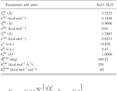
where qiand qjrepresent the partial charges of the hydrogen or oxygen atoms of two different water molecules within the cutoff distance. The parameters used in the F3C water model are given in Table I.22
This study employs the algorithm proposed in Ref. 23, in which the Lorentz forces acting on the charged particles are considered, to simulate the movement of the charged par- ticles in the homogeneous external magnetic field. A charged particle performs Larmor oscillations of Larmor frequency when the magnetic field is applied. The algorithm23describes a charged particle exposed to a static homogeneous external magnetic field which moves spirally with Larmor frequency.
In a strong magnetic field, the algorithm can be derived using a Taylor expansion of the second-order velocity Verlet algo- rithm or from a velocity transformation. Since the time step in the present simulations is sufficiently small, this study adopts the simpler form of the algorithm presented in Ref.
23, in which the strength of the magnetic field is dependent on the value of the time step. The magnetic field is assumed to act in the z direction in the simulation boxes, and the velocities of the oxygen and hydrogen atoms change in both the x and the y directions. The present simulations are based on the following:
rx共t + ⌬t兲 = rx共t兲 + ⌬tvx共t兲 +1
2共⌬t兲2关ax
C共t兲 + ⍀vy共t兲兴,
ry共t + ⌬t兲 = ry共t兲 + ⌬tvy共t兲 +1
2共⌬t兲2关ay
C共t兲 − ⍀vx共t兲兴,
rz共t + ⌬t兲 = rz共t兲 + ⌬tvz共t兲 +1
2共⌬t兲2azC共t兲,
TABLE I. Parameters of F3C water model.
Parameters and units H2O – H2O
r0OO共Å兲 3.5532
OO共kcal mol−1兲 0.1848
r0HH共Å兲 0.9000
HH共kcal mol−1兲 0.01
r0OH共Å兲 1.7883
OH共kcal mol−1兲 0.0423
qO共e.u.兲 −0.820
qH共e.u.兲 0.41
b0OH共Å兲 1.0000
0HOH共deg兲 109.47
KbOH共kcal mol−1Å−2兲 250
KHOH共kcal mol−1rad−2兲 60
vx共t + ⌬t兲 = vx共t兲 +1 2⌬t关ax
C共t兲 + ax
C共t + ⌬t兲 + 2⍀vy共t兲兴
+ 1
4共⌬t兲2⍀关ay C共t兲 + ay
C共t + ⌬t兲 − 2⍀vx共t兲兴,
vy共t + ⌬t兲 = vy共t兲 +1 2⌬t关ay
C共t兲 + ay
C共t + ⌬t兲 + 2⍀vx共t兲兴
−1
4共⌬t兲2⍀关ax C共t兲 + ax
C共t + ⌬t兲 + 2⍀vy共t兲兴,
vz共t + ⌬t兲 = vz共t兲 +1 2⌬t关az
C共t兲 + az
C共t + ⌬t兲兴,
where aCrepresents the accelerations which are independent of the velocities of the atoms and the Larmor frequency and
⍀=qB/m is determined by the magnetic field B.
In the present simulations, the strength of the magnetic field ranges from 1 to 10 T. Initially, the computational pro- cedure assumes a zero magnetic field effect and is run for 40 ps to obtain an equilibrium temperature of 300 K. The magnetic field is then applied from 40 to 140 ps simulation time.
III. RESULTS AND DISCUSSION
Electric fields break or distort the hydrogen-bond angle by causing a reorientation of the water molecules, and hence weaken or destroy the hydrogen-bond network.24This effect is the reverse of that which occurs under a magnetic field;
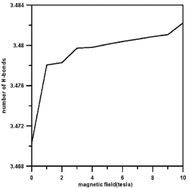
i.e., the hydrogen bonding is enhanced. The influence of the magnetic field on hydrogen bonding is shown in Fig. 1. As described previously, the structure of the water molecules is more ordered and stable under an applied magnetic field. In
determining the average number of H bonds, the present study adopts the geometric criterion25 that a hydrogen bond will be formed if the distance between the oxygen and hy- drogen atoms of a pair of water molecules is less than the first minimum of the F3C O–H radial distribution共2.4 Å兲.22 The simulation results presented in Fig. 1 indicate that the number of hydrogen bonds increases when a magnetic field is applied. Specifically, as the strength of the magnetic field increases from 1 to 10 T, the number of hydrogen bonds in- creases by approximately 0.34%. This slight increase in the number of hydrogen bonds indicates that the magnetic field enhances the water networking ability. Water clusters 共even with random arrangements兲 have equal hydrogen bonding in all directions. The higher number of hydrogen bonds implies that the size of the water cluster increases under a magnetic field, and hence the structure of the water molecules becomes more compact. The present results showing an increased number of hydrogen bonds are consistent with the findings presented by Hosoda et al.10who suggested that the enhance- ment of the hydrogen-bond strength under a high magnetic field is caused by the increased electron delocalization of the hydrogen-bonded molecules. Furthermore, the effect of the magnetic field in increasing the number of hydrogen bonds is consistent with a weakening van der Waals bonding force between the water molecules under a magnetic field11and the suppression of thermal motions as a result of the tighter hy- drogen bonding induced by the Lorentz forces.12Addition- ally, the increased number of hydrogen bonds implies that there are more water molecules forming hydrogen bonds.
However, the structure of the liquid water is still unclear.
The radial distribution functions, gO–H, gO–O and gH–H, are commonly used to examine the structure of liquid water.
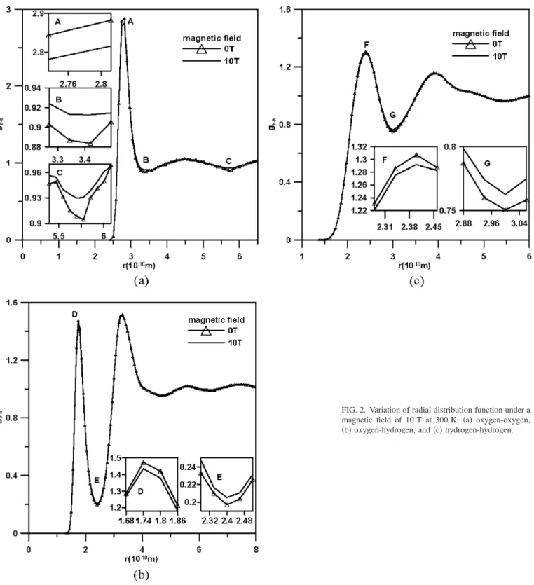
The structural differences of pure liquid water with and with- out the application of an external magnetic field of 10 T are shown in Fig. 2. Figure 2共a兲 presents the radial distribution function共gO–O兲, i.e., the distribution of the interoxygen dis- tances in any direction from a central water molecule, at 300 K under a magnetic field of 10 T. The first peak 共A兲 occurs at 2.8 Å, which corresponds to the oxygen-oxygen distance between the two hydrogen-bonding water mol- ecules. The second peak indicates the tetrahedral structure of the near neighbors and corresponds to the distance between two oxygen atoms belonging to two water molecules which are both hydrogen bonded to a third water molecule. When the strength of the magnetic field is increased to 10 T, the insets in Fig. 2共a兲 show that the height of the first peak 共A兲 decreases slightly, while the heights of the first and second valleys共i.e., B and C兲 increase. However, the positions of the first peak 共A兲 and the first valley 共B兲, i.e., 2.8 and 3.2 Å, respectively, are unchanged, indicating that the average tet- rahedral hydrogen-bonding length and the distance between two oxygen atoms belonging to two next-nearest neighbors are not influenced by the increased magnetic field. The in- creased heights of the first and second valleys under the ex- ternal magnetic field indicate that more water molecules ex- ist between the water shells. This enhanced connectivity between the water shells is also evident in Fig. 2共b兲, which illustrates the O–H radial distribution function 共RDF兲 at 300 K under a magnetic field of 10 T. Under this magnitude
FIG. 1. Variation of number of hydrogen bonds under magnetic fields with magnitudes ranging from 0 to 10 T at 300 K.
of magnetic field, the first peak 共D兲 at approximately 1.8 Å decreases, while the first valley共E兲 at 2.4 Å increases. The slight increase in the height of the first valley共E兲 indicates that more water molecules are located between the water shells. This implies that the magnetic field reforms the struc- ture of the liquid water and forces more water molecules between the water shells, hence enhancing the connectivity between them and improving the stability of the water-water network. Consequently, a small increase in the number of hydrogen bonds is apparent under a magnetic field of 10 T.
According to the results presented in Figs. 2共a兲 and 2共b兲, the water molecules tend to form more stable connections with
other water molecules in all directions. Figure 2共c兲 illustrates the H–H RDF at 300 K under a magnetic field of 10 T. It can be seen that the value of the first peak共F兲 decreases and the value of the first valley共G兲 increases under the effect of the magnetic field. In summary, the results presented in Fig. 2 demonstrate that magnetic fields enhance the bonding be- tween water molecules and stabilize the structure of liquid water.
This study also examines the self-diffusion coefficients of water molecules under a magnetic field. Studying the transport properties of liquid water is an important topic, both in fundamental science and in its applications. The mo-
FIG. 2. Variation of radial distribution function under a magnetic field of 10 T at 300 K:共a兲 oxygen-oxygen, 共b兲 oxygen-hydrogen, and 共c兲 hydrogen-hydrogen.
bility of water molecules is indicated by the value of the self-diffusion coefficient, which depends on the temperature,22 pressure, structure, and so on. Recently, sev- eral studies have investigated the self-diffusion coefficient of water molecules in different environments, including water molecules confined in a carbon nanotube,26between parallel plates,27and in sodium chloride solutions.28The value of the self-diffusion coefficients can be obtained from the Einstein relation based on the mean-square displacement function.
The results of Figs. 1 and 2 have shown that a static mag- netic field enhances the stability of water molecules, and hence influences their mobility. Calculating the self-diffusion coefficient of the water molecules provides a clearer under- standing of this change in mobility. Figure 3 presents the profiles of the self-diffusion coefficient under various mag- netic strengths. It is clear that the self-diffusion coefficient reduces as the strength of the magnetic field increases. The decreasing self-diffusion coefficient indicates that the mobil- ity of the water molecules decreases when a magnetic field is applied. If the mobility of the water molecules changes, the physical properties of the water molecules, e.g., the viscosity, thermal conductivity, and melting point, also change. Even in a high magnetic field共10 T兲, the value of the self-diffusion coefficient of liquid water is approximately 1.9
⫻10−9m2 s−1, whereas that of liquid water at 273 K without an applied magnetic field is 1.6⫻10−9m2 s−1. Although the reduction of the self-diffusion coefficient caused by the mag- netic field is not large, it nevertheless indicates a change in the properties of the liquid water.
From the results presented in Figs. 1 and 3 which show an increasing number of hydrogen bonds and a decreasing self-diffusion coefficient as the magnetic field strength is in- creased, it can be surmised that a static magnetic field re- stricts the movement of water molecules and changes the
viscosity of liquid water. These conclusions are consistent with the assumptions reported by Ishii et al.15
IV. CONCLUSION
This study has examined the effect of a static magnetic field on liquid water at an equilibrium temperature of 300 K.
It has been shown that an external magnetic field influences the number of hydrogen bonds, the structure of liquid water, and the self-diffusion coefficient of water molecules. In this study, the strength of the external magnetic field was in- creased from 0 to 10 T. The corresponding number of hy- drogen bonds was found to increase by approximately 0.34%, indicating the formation of larger water molecule clusters. In other words, it is apparent that an applied electric field and an external magnetic field exert opposite effects on the number of hydrogen bonds. Specifically, an electric field breaks the hydrogen-bond network, while a magnetic field enhances the hydrogen-bonding ability. The magnetic field induces a tighter bonding between the water molecules and improves the stability of liquid water. Under the effect of the magnetic field, the structure of the liquid water changes and more water molecules are forced between the water shells.
These molecules connect the shells and hence create a more stable water-water network. The transport properties of the water molecules, as indicated by the self-diffusion coeffi- cient, are of considerable interest in many applications. The current simulation results have shown that the self-diffusion coefficient reduces when a magnetic field is applied. In other words, the magnetic field constrains the movement of the water molecules, and hence changes both the thermal con- duction and the viscosity in the liquid state.
1J. Nakagawa, N. Hirota, K. Kitazawa, and M. Shoda, J. Appl. Phys. 86, 2923共1999兲.
2S. H. Lee, M. Takeda, and K. Nishigaki, Jpn. J. Appl. Phys., Part 1 42, 1828共2003兲.
3M. Iwasaka and S. Ueno, J. Appl. Phys. 83, 6459共1998兲.
4K. X. Zhou, G. W. Lu, Q. C. Zhou, and J. H. Song, J. Appl. Phys. 88, 1802共2000兲.
5S. N. Hakobyan and S. N. Ayrapetyan, Biofizika 50, 265共2005兲.
6N. Hirota, Y. Ikezoe, H. Uetake, J. Nakagawa, and K. Kitazawa, Mater.
Trans., JIM 41, 976共2000兲.
7A. Sugiyama, S. Morisaki, and R. Aogaki, Mater. Trans., JIM 41, 1019 共2000兲.
8V. D. Aleksandrov, A. A. Barannikov, and N. V. Dobritsa, Inorg. Mater.
36, 895共2000兲.
9G. Bikul’chyus, A. Ruchinskene, and V. Deninis, Prot. Met. 39, 443 共2003兲.
10H. Hosoda, H. Mori, N. Sogoshi, A. Nagasawa, and S. Nakabayashi, J.
Phys. Chem. A 108, 1461共2004兲.
11R. V. Krems, Phys. Rev. Lett. 93, 013201共2004兲.
12H. Inaba, T. Saitou, K. Tozaki, and H. Hayashi, J. Appl. Phys. 96, 6127 共2004兲.
13J. Lielmezs and H. Aleman, Thermochim. Acta 20, 219共1977兲.
14E. Viswat, L. K. F. Hermans, and J. J. M. Beenakker, Phys. Fluids 25, 1794共1982兲.
15K. Ishii, S. Yamamoto, M. Yamamoto, and H. Nakayama, Chem. Lett.
2005, 874.
16S. B. Zhu, J. B. Zhu, and G. W. Robinson, Phys. Rev. A 44, 2602共1991兲.
17M. Kiselev and K. Heinzinger, J. Chem. Phys. 105, 650共1996兲.
18J. M. Haile, Molecular Dynamics Simulation共Wiley, New York, 1992兲.
19M. P. Allen and D. J. Tildesley, Computer Simulation of Liquid共Claren- don, Oxford, 1991兲.
20M. Tuckerman and B. J. Berne, J. Chem. Phys. 97, 1990共1992兲.
21D. Frenkel and B. Smit, Understand Molecular Simulation 共Academic, FIG. 3. Variation of self-diffusion coefficient as magnetic field increases
from 0 to 10 T at 300 K.
San Diego, 1996兲.
22M. Levitt, M. Hirshberg, R. Sharon, K. E. Laidig, and V. Daggett, J. Phys.
Chem. B 101, 5051共1997兲.
23Q. Spreiter and M. Walter, J. Comput. Phys. 152, 102共1999兲.
24M. Kiselev and K. Heinzinger, J. Chem. Phys. 105, 650共1996兲.
25I. Benjamin, J. Chem. Phys. 97, 1432共1992兲.
26Y. Liu and Q. Wang, Phys. Rev. B 72, 085420共2005兲.
27S. P. Ju, J. G. Chang, J. S. Lin, and Y. S. Lin, J. Chem. Phys. 122, 154707 共2005兲.
28S. Koneshan and J. C. Rasaiah, J. Chem. Phys. 113, 8125共2000兲.