建立在伽瑪散度下穩健模型的調整參數之選取

國立臺灣大學理學院應用數學科學研究所 碩士論文

Institute of Applied Mathematical Sciences College of Science

National Taiwan University Master Thesis

建立在伽瑪散度下穩健模型的調整參數之選取 Robust Model Fitting - Selection of Tuning Parameters in

the Aspect of Gamma Clustering

蕭奕 Yi Hsiao

指導教授：杜憶萍博士 Advisor: I-Ping Tu, Ph.D.

中華民國 107 年 6 月 June, 2018

誌謝

感謝指導教授杜憶萍老師，讓我在大學的時候接觸統計這個領域，

並因此對統計產生興趣，走上研究的道路。雖然路途上遭遇許多困難，

但每次和老師討論時，能學習到用各種方式去看待不同問題，並找出 問題的關鍵點，再加上不時的鼓勵，讓我一步一步幸運且順利地完成 論文。

感謝大學及研究所的師長們，讓我在求學生涯中打下扎實的數學基 礎。

感謝陪我唸書、一起討論課業準備考試的同學們，以及協助我完成 論文和準備口試的學長姐，有你們陪伴學習更加有趣。

最後感謝我的父母，對我的決定總是給予支持，讓我更專注於課 業。儘管不常回家，但總會讓我知道家永遠是最好的避風港。

摘要

Windham 在 1995 年的論文 Robustifying Model Fitting 提出權重分布 方法，解決在存有異常數據情況下可有效的估計均值，這個權重分布 使用了一個參數，這個參數會影響到均值的估計表現。Windham 同時 提出此參數的選取方法，但我們發現在一些數值模擬例子中，這個參 數選取方法表現並不佳。我們提出另一個選取方法，在數值模擬上有 較佳的表現。除了一般的均值估計，我們也成功地把此方法應用在群 聚分析。

關鍵字： 穩健估計、影響函數、伽瑪散度、群聚分析

Abstract

In 1995, Windham came out with an idea of weighted distribution in his thesis, Robustifying Model Fitting, and he used the idea to find a mean esti- mator when there are outliers in the original data. There is a tuning parameter in this estimator, and selecting the parameter will affect the mean estimate in the same data. In the same thesis, he also suggested a criterion of selecting the tuning parameter, but we found out that this criterion wasn’t doing well in some simulations. Considering the problem, we propose another criterion which can derive a better mean estimator. Besides, we can also apply this method to clustering problem.

Keywords: robust estimate, influence function, gamma-divergence, cluster- ing

Contents

口試委員會審定書 iii

誌謝 v

摘要 vii

Abstract ix

1 Introduction 1

1.1 What is Robust? . . . 1

1.2 How to get Robust? . . . 3

1.2.1 M-estimator . . . 4

1.2.2 Weighted data . . . 5

1.3 Why need to do this question? . . . 6

2 Literature Review 9 2.1 Normal Robust Model . . . 9

2.2 General Description . . . 10

2.3 Selection Criterion . . . 12

2.4 γ-estimate and Weighted Robustified estimate . . . 14

2.4.1 Some Notes about γ-clust . . . 14

2.4.2 Weighted Distribution . . . 15

3 Our Selection Criterion 17

3.2 g_θ is bivariate normal, θ = µ . . . 19

3.3 g_θ is univariate normal, θ = (µ, σ²)^T . . . 20

3.4 gθ is qGaussian, θ = µ . . . 21

3.4.1 Some Notes about qGaussian . . . 21

3.4.2 Weighted Distribution . . . 23

3.4.3 Applied to gamma-clust . . . 24

4 Numerical Examples 27 4.1 One Dimension Case . . . 27

4.1.1 One component with outliers . . . 27

4.1.2 Five components . . . 31

4.2 Two Dimension-One Component with Outliers . . . 31

4.3 Variance Unknown . . . 32

4.4 qGaussian Model . . . 33

Bibliography 37

List of Figures

1.1 median, mean, robustified mean . . . 2

1.2 Score function of estimator, assuming the location parameter is 0. . . 5

4.1 . . . 27

4.2 . . . 29

4.3 . . . 29

4.4 . . . 30

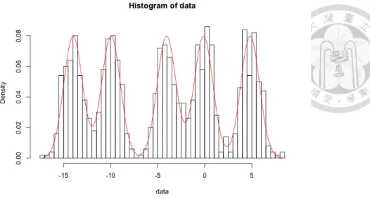
4.5 Red curve is the estimated density. . . 32

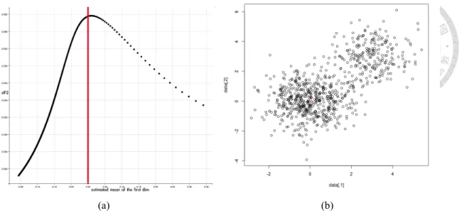
4.6 Result of 2-dim data. (a) mean of the first dimension and sIF2. (b) scatter plot and the estimated mean (red triangle). . . 33

4.7 Variance unknown simulation. (a) estimated mean and sIF2. (b) estimated variance and sIF2. . . 34

List of Tables

2.1 Estimates for ˆµ and ˆσ² . . . 10

4.1 Result of First Example . . . 28

4.2 Comparing data in first example . . . 28

4.3 Result of Second Example . . . 30

4.4 Comparing data in second example . . . 31

4.5 Result of 1-dim clustering . . . 32

4.6 Result of qGaussain model . . . 33

4.7 Comparing ˆµ and ˆµtrim . . . 34

Chapter 1 Introduction

1.1 What is Robust?

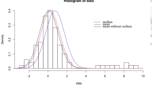
Maximum likelihood estimate (MLE) or method of moments are most common way to estimate parameter. Under some regularity conditions, maximum likelihood estimator is consistent. That is, the probability of the estimator converging to the true parameter is 1, as the number of samples goes to infinity. However, finite sample or outliers may hinder the consistent property of the estimate. We can think this through the fundamental spirit of maximizing the likelihood. The likelihood function is defined as the product of the density of the observed data (assume i.i.d.) including outliers. Considering this, it is unreasonable to maximize the likelihood for those outlier terms. And if there are more outliers or the outliers are further far away from the true data, the influence on the estimator become larger. For example, considering a normal distribution model, the maximum likelihood estimator for mean is the sample mean. This estimator can become arbitrary large if we add distant data points in the sample (Figure 1.1). Thus, we say that sample mean is not robust. Another common mean estimator, median, needs over half of the data points to have effect on the estimator, hence is robust. We may want to know how many portions of data can influence the estimator, or how much a data point influence the estimator, thus following are some measurements often used for quantify robustness.

Figure 1.1: median, mean, robustified mean

Measurement of Robustness

• Influence function (Hampel, 1968) is defined as

IF (x; T, F ) = lim

ε→0

T{(1 − ε)F + εδ^x} − T (F )

ε ,

where F is the distribution function, T (F ) is the parameter estimator, and δx(u) is a heaviside step function, which is 0 when u < x, and is 1 otherwise.

This definition means that we perturbate the distribution at a point x, and have in- terest in the variation rate of the estimator.

• Gross-error sensitivity is defined as

γ^∗(T, F ) = sup

x |IF (x; T, F )|,

γ^∗(T, F ) is the supreme of the absolute value of influence function, which measures the worst influence a data point can make on the estomator.

• Breakdown point is defined as

ε^∗ = inf{ε : sup

x |T (F ) − T (F^ε)| = ∞}, where F_ε = (1− ε)F + εδx.

Let’s give an example. Suppose F is the distribution, then sample mean can be expressed as T (F ) =!

udF . Hence the influence function of T (F ) is

IF (x; T, F ) = lim

ε→0

T{(1 − ε)F + εδ^x} − T (F ) ε

= lim

ε→0

! ud((1− ε)F + εδx)−! udF ε

= lim

ε→0

ε!

udδx− ε! udF

ε = x− T (F )

The gross-error sensitivity is

γ^∗(T, F ) = sup

x ∥IF (x; T, F )∥ = sup

x ∥x − T (F )∥ = ∞, which is the worst case in the view of robustness.

And the breakdown point of sample mean is

ε^∗ = inf{ε : sup

x |T (F ) − T (Fε)| = ∞} = inf{ε : sup

x |ε(x − T (F ))| = ∞} = 0, which is also the worst case.

Now, we figure out that sample mean is not robust, so next section is some ideas to get robust.

1.2 How to get Robust?

One way to get robust is to improve maximum likelihood estimator, since it is maximum likelihood type, we called it M-estimator.

1.2.1 M-estimator

• MLE: min"

− log f(xi; θ), where f is the density function.

Generalized MLE: min"

p(xi; θ), where p can be any function.

• If p(x; θ) is differentiable with respect to θ, then the M-estimator is to solve

E_F[ψ(x; θ)] = 0,

where ψ(x; θ) = ^∂p(x;θ)_∂θ is the score function.

• The influence function of the M-estimator

Let T (F ) be the M-estimator with E_F[ψ(x; T (F ))] = 0, for all distributions F . Hence,

EFε[ψ(x; T (Fε))] = 0

To derive influence function, take derivative with respect to ε,

∂

∂εEFε[ψ(x; T (Fε))] = 0

⇒ _∂ε^∂ !

ψ(u; T (Fε))d((1− ε)F (u) + εδx) = 0

If the integration and differentiation can be interchanged, then

⇒! _∂

∂ε{ψ(u; T (F^ε))d((1− ε)F (u) + εδ^x)} = 0

⇒! #_∂

∂ε{ψ(u; T (F^ε))}d((1 − ε)F (u) + εδ^x) + ψ(u; T (Fε))d(_∂ε^∂{(1 − ε)F (u) + εδ^x})$

= 0

⇒! # _∂

∂θ[ψ(u; θ)]θ=T (Fε)dFε(u)·_∂ε^∂[T (Fε)] + ψ(u; T (Fε))d(δx− F (u))$

= 0

⇒! # _∂

∂θ[ψ(u; θ)]θ=T (F )dF (u)· _∂ε^∂[T (Fε)]ε=0+ ψ(u; T (F ))d(δx− F (u))$

= 0 Note that _∂ε^∂[T (Fε)]ε=0 = IF (x; T, F ) and

! ψ(u; T (F ))d(δx− F (u)) = ψ(x; T (F )), we have IF (x; T, F ) = ψ(x;T (F ))

−! _∂

∂θ[ψ(u,θ)]θ=T (F )dF (u)

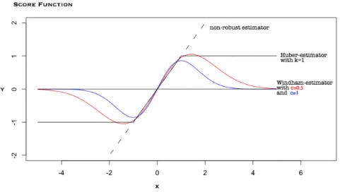
Figure 1.2 shows various score functions of location estimators θ, and θ = 0.

Huber estimator (1964) is an M-estimator with score function ψk(x; θ) = max(−k, min(k, x−

θ)), the black line is for k = 1. And Windham estimator (1995) is also an M-estimator with ψ_c(x; θ) = √

c + 1 exp(−^c(x− θ)²)(x− θ), the red curve is for c = 0.5 and blue

curve is for c = 1.

For different function p(x; θ) or ψ(x; θ), the estimator derived has different robustness.

This property can be implicated by Figure 1.2, traditional score function of MLE ψ(x; θ) = x− θ, the dashed line, counts every point x and going to arbitrary large when x goes to infinity, while other robustified estimators don’t.

Figure 1.2: Score function of estimator, assuming the location parameter is 0.

1.2.2 Weighted data

Another way to get robust is to weight the data such that the point more likely to happen has higher weight, and less likely to happen has lower weight. So, thinking a weight with such property, one can immediately came up with density function, and Windham gave an extra exponent c to the power of the density function. For example, data {x1, x2, ..., xn} are from normal distribution F with mean 0 and unknown variance θ, then its weight function is

w(xi; θ) = Kφ^c(xi; θ),

where φ is the normal density function with mean 0 in the model, c is a fixed exponent term, K is a constant so that the sum of weight is 1.

Hence, the weighted sample variance is

v =

%n i

w(xi; θ)x²_i

And the weighted population variance is

v^∗ =

&

x²w^∗(x; θ)φ(x; θ)dx,

where

w^∗(x; θ) = K^∗φ^c(x; θ), (1.1) K^∗ = [!

φ^c(x; θ)dF ]⁻¹ = E_F[φ^c(x; θ)]⁻¹ is a constant. In this model dF = φ(x; θ)dx, hence!

w^∗(x; θ)dF = !

w^∗(x; θ)φ(x; θ)dx = 1. Notice that w^∗(x; θ)φ(x; θ), called the weighted density function, and is same as the normal density with mean 0 and variance v^∗ = θ/(c + 1). If the model is correct, v^∗ and v should be close. Thus, using these relations, we can derive the robust estimate of parameter θ.

Also, there is a exponent term c, which can adjust weight and hence called tuning param- eter. Windham (1995)[3] studied in how to select this parameter and called this method Robust Model Fitting. In this thesis, we propose another method of selection and do re- search with it.

1.3 Why need to do this question?

Past robust model, such as Huber estimate (1964)[2], Windham (1995)[3] estimate, and Akifumi Notsu, Shinto Eguchi (2016)[1] Gamma-clust robust estimate, there are tuning parameters. Tuning parameters will affect the robustness of the model (Figure 1.2). In Windham’s model, parameter c determines the weight of each point. Selection of c is im- portant when doing clustering analysis, since larger the c becomes, more robust the model will be, and number of clusts will closer to the number of data points; on the contrary, smaller the c becomes, less robust the model will be, and number of clusts will go to 1.

In general, there is a reasonable interval to choose the parameter, and usually is selected

subjectively. By using influence function and Fisher information, we give a objective selection criterion, and more details can be seen in chapter 3.

Chapter 2

Literature Review

2.1 Normal Robust Model

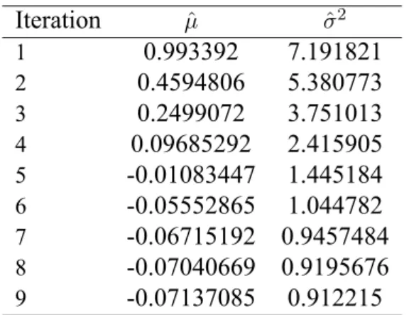
We use a simple example to elaborate Windham’s iterative algorithm estimates. Assume there are 400 samples {x1, x2, ..., x400}, and among of them, there are 340 samples are from N(µ, σ²), µ = 0, σ² = 1 and the rest are outliers around µ^∗ = 7. We want to estimate µ and variance σ².

• First step : Find initials.

Use sample mean and sample variance (MLE in normal distribution) as initials.

ˆ

µ = ¯x = 0.99, ˆσ² = ₄₀₀¹ "

(xi− ¯x)² = 7.19

• Second step : Weight data.

wi = w(xi, ˆµ, ˆσ²) = Kφ^c(xi; ˆµ, ˆσ²), c is chosen to be 0.37, φ is normal density function, and K is a constant such that"400

i=1wiis 1.

Similarly, we use MLE on the weighted data, and get, ˆ

m ="

w_ix_i = 0.45, ˆs² ="

w_i(x_i− ˆm)² = 3.93

• Third step : Find the non-weighted parameters such that we can get ˆm and ˆs² in second step after weighting.

That is, if the model is correct, which is satisfied normal distribution with den-

Iteration µˆ σˆ²

1 0.993392 7.191821

2 0.4594806 5.380773

3 0.2499072 3.751013

4 0.09685292 2.415905

5 -0.01083447 1.445184

6 -0.05552865 1.044782

7 -0.06715192 0.9457484 8 -0.07040669 0.9195676

9 -0.07137085 0.912215

Table 2.1: Estimates for ˆµ and ˆσ².

is φ(x; µ, σ²/(c + 1)). Thus, we can revise the new parameters to ˆµ+ = ˆm = 0.45, ˆσ₊² = 1.37ˆs² = 5.38.

• Fourth step : Repeat step 1 to 3, until the estimates converge. In other words, replace ˆ

µ and ˆσ²by new estimates ˆµ+and ˆσ₊² until they converge (Table 2.1).

2.2 General Description

We now use mathematical way to describe the example above. In the beginning, we ob- serve that there are n one dimension data, {x1, x2, ..., xn} from the distribution F , and its empirical distribution is ˆF . T ( ˆF ) is a parameter estimator, and T ( ˆF ) = (¯x,_n¹ "

(xi− ¯x)²) is the maximum likelihood case. And note that T (F ) satisfies E_F[ψ(x; T (F ))] = 0, where ψ is the score function of T (F ). Moreover, Windham defined weighted distribution as dFc,t(x) = w^∗(x; t)dF (x), where w^∗(x; t) = K^∗g^c(x; t), g is the density in the model, K^∗ = {E^F[g^c(x; t)]}⁻¹, and here we assume g is normal. If we plug ˆF into F , then d ˆFc,t(x) = ˆw^∗(x; t)d ˆF (x), where ˆw^∗(x; t) = ˆK^∗g^c(x; t), and ˆK^∗ ={E^ˆ[g^c(x; t)]}⁻¹.

Hence, the second step is,

T ( ˆFc,t) = ( ˆm, ˆs²) = (

&

xd ˆFc,t,

&

(x− ˆm)²d ˆFc,t)

= (

&

ˆ

w^∗(x; t)xd ˆF ,

&

ˆ

w^∗(x− ˆm)²d ˆF )

= (1 n

% g^c(x_i; t)

1 n

"

g^c(x_j; t)xi, 1 n

% g^c(x_i; t)

1 n

"

g^c(x_j; t)(xi − ˆm)²)

= (%

wixi,%

wi(xi− ˆm)²),

where w_i = w(xi; t) = ^"gc_g^(xc(x^i;t)j;t).

Next, we want to know the difference of the estimates between the weighted model and non-weighted one. Hence, assume that the normal density of F is g(x; µ, σ²), We have,

&

w^∗(x; µ, σ²)xdF =

! g^c+1(x; µ, σ²)xdx

! g^c+1(x; µ, σ²)dx = µ

&

w^∗(x; µ, σ²)(x− ˆm)²dF =

&

w^∗(x; µ, σ²)(x− µ)²dF

=

! g^c+1(x; µ, σ²)(x− µ)²dx

! g^c+1(x; µ, σ²)dx

= σ² (c + 1)

From the formula above, we know that mean is unchanged and the variance is multiplied by _(c+1)¹ in the weighted model. Therefore, a function τ is defined to transform the esti- mator between weighted and non-weighted distribution,

( ˆm, ˆs²) = τ (ˆµ+, ˆσ²₊) = (ˆµ+, ˆσ²₊/(1 + c))

(ˆµ+, ˆσ²₊) = τ⁻¹( ˆm, ˆs²) = ( ˆm, (1 + c)ˆs²) For N ≥ 0, t⁽⁰⁾ = T ( ˆF ),

t^{(N +1)} = τ⁻¹{T ( ˆF )}

is an iterative procedure. And the Windham robustified estimate (WRE) T_c( ˆF ) is hence defined as T_c( ˆF ) = ˆθ, where ˆθ is the estimate from the last iteration.

2.3 Selection Criterion

Tcis a solution of EF[w^∗(x; θ)ψ(x; τ (θ))] = 0, hence is an M-estimator, the corresponding score function is

ψc(x; θ) = w^∗(x; θ)ψ(x, τ (θ)) (2.1) Let h(t) = τ⁻¹{T (F^c,t)}, if the process converges, we will have h(θ) = θ. Hence,

EFc,t[ψ[x; τ{h(t)}]] = 0

Take derivative with respect to t, and derive the convergence rate h^′(t).

∂

∂tEFc,t[ψ[x; τ{h(t)}]] = 0

⇒ ∂

∂tEF[w^∗(x; t)ψ[x; τ{h(t)}]] = 0

⇒ E^F[ '∂

∂tw^∗(x; t) (

ψ[x; τ{h(t)}] + w^∗(x; t) '∂

∂tψ[x; τ{h(t)}]

( ] = 0

⇒ EF[cw^∗(x; t)(∂

∂tlog g(x; t))ψ(x; τ(h(t)))] + E_F[w^∗(x; t)∂ψ(x; τ (h(t)))

∂τ (h(t))

∂τ (h(t))

∂h(t)

∂h(t)

∂t ] = 0 where _∂t^∂w^∗(x; t) = cw^∗(x; t)(_∂t^∂ log g(x; t))

When it is about to converge, i.e. h(t) = t,

h^′(t) =−c{EFc,t[∂ψ(x; τ (t))

∂τ (t) ]∂τ (t)

∂t }⁻¹EFc,t[ψ(x; τ (t))∂

∂t(log g(x; t))]

=−cEF[_∂t^∂(log g(x; t))ψc(x; t)]

EF[w^∗(x; t)∂ψ(x;τ (t))

∂τ (t)

∂τ (t)

∂t ]

= −cE^F[_∂t^∂(log g(x; t))ψc(x; t)]

EF[ψ^′_c(x; t)]− EF[cw^∗(x; t)_∂t^∂(log g(x; t))ψ(x; τ (t))]

= −cE^F[_∂t^∂(log g(x; t))ψc(x; t)]EF[ψ^′_c(x; t)]⁻¹ I− cEF[_∂t^∂(log g(x; t))ψc(x; t)]EF[ψ_c^′(x; t)]⁻¹

= cB(t){I + cB(t)}⁻¹,

Since

ψ_c^′(x; t) = ∂

∂t(ψc(x; t)) = cw^∗(x; t)(∂

∂tlog g)ψ(x; τ(t)) + w^∗(x; t)∂ψ(x; τ (t))

∂τ (t) τ^′, (2.2) where B(t) = −EF[_∂t^∂(log g(x; t))ψc(x; t)]EF[ψ_c^′(x; t)]⁻¹, which is related to influence function. In fact,

B{T^c(F )} = E^F[−E^F[ψ^′_c(x; t)|^t=Tc(F )]⁻¹ψc(x; Tc(F ))· ∂

∂t(log g(x; t))|^t=Tc(F )]

= EF[IF (x; Tc, F )s(x; Tc(F ))],

where IF (x; T_c, F ) =−EF[ψ^′_c(x; t)|t=Tc(F )]⁻¹ψ_c(x; T_c(F )) is the influence function and s(x; T_c(F )) = _∂t^∂(log g(x; t))|t=Tc(F )is the score function.

According to Cauchy–Schwarz inequality,

{EF[s²(x; Tc(F ))]EF[IF²(x; Tc, F )]}⁻¹ ≤ B⁻²{Tc(F )}

And Windham noted that the left hand side is just the asymptotic relative efficiency, which is the reciprocal of the Fisher information times the asymptotic variance. Hence, he used B⁻²as a criterion for choosing c, which is

ρ(c) = B⁻²{Tc(F )}

By h^′(t) = cB(t){I + cB(t)}⁻¹,

ρ(c) = (c/h^′(t)− c)²

Thus, the tuning parameter c is chosen by

ˆ

c = arg max

c ρ(c)

In simulation, the convergence rate h^′(t) can be estimated by_|t^|t(N^{(N )}−1)^−t−t^{(N(N−1)−2)|}|, and this is the method Windham used.

2.4 γ-estimate and Weighted Robustified estimate

2.4.1 Some Notes about γ-clust

• γ-divergence

Like K-L divergence, is a measure of the difference between two probability distri- butions.

• γ-cross entropy

Suppose {x1, x₂, ..., x_n} are from the distribution with density f. And there is a density gθ we assumed that it is the model density with θ unknown. The γ-cross entropy dγ(f, gθ) is defined as

dγ(f, gθ) = −1 γ log{

&

g(x; θ)^γf (x)dx} + 1 1 + γ log

&

g(x; θ)^1+γdx

dγ(f, gθ) can be empirically estimated by

dγ( ˆf , gθ) =−1 γ log{1

n

%n i=1

g(xi; θ)^γ} + 1 1 + γ log

&

g(x; θ)^1+γdx,

where ˆf is the empirical pdf.

The small value of γ-cross entropy means two distributions are close, so the robust estimator ˆθ_γcan be defined by minimizing d_γ( ˆf , g_θ), i.e.

θˆγ = arg min

θ dγ( ˆf , gθ)

We substitute g_θ to g(x; µ, Σ), where g is a p-variate normal density function.

dγ( ˆf , g(x; µ, Σ)) =−1 γ log{1

n

%n

g(xi; µ, Σ)^γ} + 1 1 + γ log

&

g(x; µ, Σ)^1+γdx

⇒ e^{−dγ( ˆ}f ,g(x;µ,Σ)) ={1 n

%n

g(xi; µ, Σ)^γ}^1/γ{

&

g(x; µ, Σ)^1+γdx}^−1+γ1

Note that

&

g(x; µ, Σ)^1+γdx =

&

{(2π)^−p2(detΣ)⁻¹² exp (−1

2(x− µ)^TΣ⁻¹(x− µ))}^1+γdx

= (2π)^−pγ2 (1 + γ)⁻¹²(detΣ)^−γ2

⇒ e^{−dγ( ˆ}f ,g(x;µ,Σ))γ = 1 n

%g(xi; µ, Σ)^γ{

&

g(x; µ, Σ)^1+γdx}^−1+γγ

= 1 n

%g(xi; µ, Σ)^γ{(2π)^−pγ2 (1 + γ)⁻¹²(detΣ)^−γ2}^−1+γγ

∝%

g(xi; µ, Σ)^γ(detΣ)^2(1+γ)γ2

Thus, we derive a function of γ which is likelihood function in γ-divergence sense.

• γ-utility function

L_γ(µ, Σ) = (detΣ)^2(1+γ)γ2

%n i=1

g(x_i; µ, Σ)^γ

Hence, the robust estimator is to maximize L_γ(µ, Σ)

2.4.2 Weighted Distribution

To maximize γ-utility function, we take derivatives with respect to µ and set it be 0. Here, g(x; µ, σ²) is univariate normal density.

∂ ∂ %

⇒ ∂"

g^γ(xi; µ, σ²)

∂µ = 0

⇒ γ%

g^γ−1(xi; µ, σ²)∂g(xi; µ, σ²)

∂µ = 0

⇒%

g^γ(xi; µ, σ²)(xi− µ) = 0

⇒ ˆµ =

"

g^γ(xi; µ, σ²)xi

"

g^γ(xi; µ, σ²)

Similarly, take derivatives w.r.t. σ²,

∂

∂σ²Lγ(µ, σ²) = ∂

∂σ²

%g^γ(xi; µ, σ²)(σ²)^2(1+γ)γ2 = 0

⇒ γ²

2(1 + γ)(σ²)^{2(1+γ)γ2 −1}%

g^γ(xi; µ, σ²) + (σ²)^2(1+γ)γ2 %

γg^γ−1(xi; µ, σ²)∂g(x_i; µ, σ²)

∂σ² = 0

⇒ γ

2(1 + γ)

%g^γ(xi; µ, σ²) + σ²%

g^γ−1(xi; µ, σ²)∂g(xi; µ, σ²)

∂σ² = 0

and since

∂g(x; µ, σ²)

∂σ² = ∂

∂σ²(2πσ²)⁻¹²e^{−(x2σ2−µ)2}

= (2π)⁻¹²(−1

2)(σ²)⁻³²e^{−(x2σ2−µ)2} + (2π)⁻¹²(σ²)⁻¹²(x− µ)²

2(σ²)² e^{−(x2σ2−µ)2}

=−1

2(σ²)⁻¹g(x; µ, σ²) + g(x; µ, σ²)(x− µ)² 2(σ²)² We have,

γ 2(1 + γ)

%g^γ(x_i; µ, σ²) +%

g^γ(x_i; µ, σ²)(−1

2 +(xi− µ)² 2σ² ) = 0

⇒ 1

1 + γ

%g^γ(xi; µ, σ²) = %

g^γ(xi; µ, σ²)(x_i− µ)² σ²

⇒ ˆσ² = (1 + γ)

"

g^γ"(xi; µ, σ²)(xi− µ)² g^γ(xi; µ, σ²)

We figure out that the estimator we derived from the aspect of γ-divergence is exactly a Windham robustified estimate.

Chapter 3

Our Selection Criterion

In this chapter, we propose another criterion to choose c. From chapter two, we knew that the criterion B⁻² is related to convergence rate of the estimates and hence can be easily calculated. However, if we look into it carefully, the true criterion is {E^F(s²)EF(IF²)}⁻¹ rather than its upper bound B⁻². Therefore, our selection criterion of the tuning parameter c is,

ˆ

c = arg max

c {EF(s²(x; Tc))EF(IF²(x; Tc, F ))}⁻¹

The following are some reasons that we prefer using {EF(s²EF(IF²))}⁻¹(denoted sIF2) as criterion:

• The true criterion is {E^F(s²)EF(IF²)}⁻¹rather than its upper bound B⁻².

• In the same model, the selection of c is stable, since we calculated the criterion directly.

• The MSE of the estimator is smaller.

• If c is large, then ρ(c) = (c/h^′(t)− c)² becomes large. That is, ρ tends to choose larger c.

• Although the convergence rate is easy to compute, it’s unstable.

In each section we discuss and calculate the criterion sIF2 under various model distri-

3.1 g

is univariate normal, θ = µ

The distribution density function g_θ(x) = g(x; µ) in this model is univariate normal with unknown mean µ and variance 1.

From eq. (1.1) w^∗(x; µ) = K^∗g^c(x; τ (µ)) and from eq. (2.1) ψ_c(x; µ) = w^∗(x; µ)ψ(x; τ (µ)), where τ(µ) = µ and ψ(x; µ) = x − µ

First, the score function is

s(x; µ) = ∂

∂µ{log g(x; µ)}

= ∂

∂µ{log 1

√2π − (x− µ)²

2 } = x − µ The Fisher information is

EFˆ(s²(x; µ)) = 1 n

%(x_i− µ)²

Second, since T_c(F ) is an M-estimator, its influence function can be written as

IF (x; Tc, F ) =−EF[ψ^′_c(x; µ)|µ=Tc(F )]⁻¹ψc(x; Tc(F ))

=−EF[cw^∗(x; Tc(F ))(x− Tc(F ))²− w^∗(x; Tc(F ))]⁻¹w^∗(x; Tc(F ))(x− Tc(F ))

= w^∗(x; Tc(F ))(x− T^c(F )) 1− cEF[w^∗(x; T_c(F ))(x− Tc(F ))²]

⇒ IF²(x; Tc, F ) = w^∗2(x; Tc(F ))(x− T^c(F ))² (1− cEF[w^∗(x; Tc(F ))(x− Tc(F ))²])² From eq. (2.2), ψ_c^′(x; µ) = cw^∗(x; µ)(x− µ)²− w^∗(x; µ) Therefore, the asymptotic variance is

EF(IF²(x; Tc, F )) = EF[w^∗2(x; Tc(F ))(x− T^c(F ))²] (1− cEF[w^∗(x; Tc(F ))(x− Tc(F ))²])²

EFˆ(IF²(x; Tc, ˆF )) = n"

w²(xi; Tc( ˆF ))(xi− T^c( ˆF ))² (1− c"

w(x; T ( ˆF ))(x − T ( ˆF ))²)²

And the asymptotic relative efficiency is

{EF^ˆ(s²(x; Tc( ˆF )))EFˆ(IF²(x; Tc, ˆF ))}⁻¹

={1−%

w(xi; Tc( ˆF ))(xi−Tc( ˆF ))}²/{%

(xi−Tc( ˆF ))²%

w²(x; Tc( ˆF ))(xi−Tc( ˆF ))²} Hence, we derived the criterion sIF2 in the model of distribution g_θ(x) is univariate normal with unknown mean µ and variance 1.

3.2 g

is bivariate normal, θ = µ

The distribution density function gθ(x) = g(x, µ) in this model is bivariate normal with unknown mean µ and variance I², where I²is a 2 by 2 identity matrix.

The Fisher information matrix is

EFˆ(s²(x; µ)) = EFˆ[(x− µ)(x − µ)^T] = ¹_n"n

i=1(xi− µ)(xi− µ)^T Robust Model Fitting part :

EF[ψ_c^′(x; µ)] = EF[cw^∗(x; µ)(x− µ)(x − µ)^T + w^∗(x; µ)(−I2)] (from eq. (2.2))

= cE_F[w^∗(x; µ)(x− µ)(x − µ)^T]− I2

EFˆ[ψ_c^′(x; µ)] = c"

w(x_i, µ)(x_i− µ)(xi− µ)^T − I2

And the influence function is

IF (x; Tc, F ) =−E^F[ψ^′_c(x; µ)|^µ=Tc(F )]⁻¹ψc(x; Tc(F )) Hence,

IF²(x; Tc, F ) =−EF[ψ^′_c(x; µ)|µ=Tc(F )]⁻¹ψc(x; µ)(−EF[ψ_c^′(x; µ)|µ=Tc(F )]⁻¹ψc(x; Tc(F )))^T

= EF[ψ_c^′(x; µ)|µ=Tc(F )]⁻¹ψc(x; Tc(F )ψc(x; Tc(F ))^TEF[ψ^′_c(x; µ)|µ=Tc(F )]⁻¹ Note that

E_F[ψ_c(x; T_c(F )ψ_c(x; T_c(F ))^T] = E_F[w^∗(x− Tc(F ))(w^∗(x− Tc(F )))^T] EFˆ[ψc(x; Tc( ˆF )ψc(x; Tc( ˆF ))^T] = "

w_i²(xi− T^c( ˆF ))(xi− T^c( ˆF ))^T, where wi is the weight for the i-th data. We have

EFˆ[IF²(x; Tc, ˆF )]

(c"

wi(xi− Tc( ˆF ))(xi− Tc( ˆF ))^T − I2)⁻¹

Finally, we derive the formula of {EF^ˆ[s²]EFˆ[IF²]}⁻¹ and we choose the reciprocal of the product of the largest eigenvalue of EFˆ[s²(x; Tc( ˆF ))] and EFˆ[IF²(x; Tc, ˆF )] as our criterion.

3.3 g

is univariate normal, θ = (µ, σ

)

The distribution density function g_θ(x) = g(x, (µ, σ²)^T) in this model is univariate nor- mal with unknown mean µ and variance σ².

The Fisher information matrix is

EF[s²(x; θ)]ij = EF[s(x; θ)(s(x; θ)^T)]ij = EF[(_∂θ^∂_ilog g(x; θ))(_∂θ^∂

j log g(x; θ))]

Here, θ = (µ, σ²)^T Hence,

EF(s(x; θ)(s(x; θ))^T) = EF

⎡

⎢⎣

(x−µ)² σ⁴

(x−µ)

σ² (−_2σ¹² +^(x_2σ^−µ)4 ²)

(x−µ)

σ² (−_2σ¹² +^(x_2σ^−µ)4²) (−_2σ¹² +^(x_2σ^−µ)4²)²

⎤

⎥⎦

ψ(x; θ) =

⎡

⎢⎣ x− µ (x− µ)²− σ²

⎤

⎥⎦

Robust Model Fitting part :

w^∗(x; θ) = ^√_c+1¹ exp(−_2σ^c2(x− µ)²)

ψc(x; θ) = w^∗(x; θ)ψ(x; τc(θ)) = w^∗(x; θ)

⎡

⎢⎣ x− µ (x− µ)²− _c+1^σ2

⎤

⎥⎦

EF[ψ_c^′(x; θ)]

= E_F

⎡

⎢⎣

∂

∂µw^∗(x; θ)(x− µ) _∂σ^∂2w^∗(x; θ)(x− µ)

∂

∂µw^∗(x; θ)[(x− µ)²− _c+1^σ2 ] _∂σ^∂2w^∗(x; θ)[(x− µ)²− _c+1^σ2 ]

⎤

⎥⎦

= EF

⎡

⎢⎣A B C D

⎤

⎥⎦

We know

∂

∂µw^∗(x; θ) = cw^∗(x; θ)x− µ σ² and

∂

∂σ²w^∗(x; θ) = cw^∗(x; θ)(x− µ)² 2σ⁴ Thus,

A = _∂µ^∂ w^∗(x; θ)(x− µ) = cw^∗(x; θ)^(x−µ)_σ2 ² − w^∗(x; θ) B = _∂σ^∂2w^∗(x; θ)(x− µ) = cw^∗(x; θ)^(x−µ)_2σ4³

C = _∂µ^∂ w^∗(x; θ)[(x− µ)²− _c+1^σ2 ] = cw^∗(x; θ)(^(x−µ)_σ2 ³ − ^x_c+1^−µ)− 2w^∗(x; θ)(x− µ) D = _∂σ^∂2w^∗(x; θ)[(x− µ)² −_c+1^σ2 ] = cw^∗(x; θ)(^(x−µ)_2σ4⁴ − _2σ^(x−µ)2_(c+1)² )− ^w∗_c+1^(x;θ) Hence, from the formula before

IF²(x; Tc, F ) =−E^F[ψ^′_c(x; θ)|θ=Tc(F )]⁻¹ψc(x; Tc(F ))(−E^F[ψ^′_c(x; θ)|θ=Tc(F )]⁻¹ψc(x; Tc(F )))^T

= EF[ψ_c^′(x; θ)|^θ=Tc(F )]⁻¹ψc(x; Tc(F ))ψc(x; Tc(F ))^TEF[ψ_c^′(x; θ)|^θ=Tc(F )]⁻¹

Thus, we derive the formula of {EF[s²]EF[IF²]}⁻¹and choose the reciprocal of the prod- uct of the largest eigenvalue of E_F[s²(x; Tc(F ))] and EF[IF²(x; Tc, F )] as our criterion.

3.4 g

is qGaussian, θ = µ

3.4.1 Some Notes about qGaussian

• β-power model pdf (qGaussian):

fβ(x; µ, Σ) = cβ(det2πΣ)⁻¹²{1 − β

2 + (p + 2)β(x− µ)^TΣ⁻¹(x− µ)}^1/β+

,where β > −2/(p + 2), x ∈ R^p

As β → 0, fβ converges to normal density.

f0(x; µ, Σ) := limβ→0fβ(x; µ, Σ)

= limβ→0cβ∥2πΣ∥⁻¹²{1 − _2/β+(p+2)¹ (x− µ)^TΣ⁻¹(x− µ)}^1/β+

= c0∥2πΣ∥⁻¹² exp(−¹₂(x− µ)^TΣ⁻¹(x− µ)), which is N (µ, Σ)

• γ-cross entropy

In section 2.4.1, we have given the form of empirical γ-cross entropy dγ( ˆf , gθ)

dγ( ˆf , gθ) = −1 γ log{1

n

%n i=1

g(xi; θ)^γ} + 1 1 + γlog

&

g(x; θ)^1+γdx

,where ˆf is the empirical pdf.

Hence, we substitute g_θ to f_β,

dγ( ˆf , fβ(x; µ, Σ))

=−1 γ log{1

n

%n

fβ(xi; µ, Σ)^γ} + 1 1 + γ log

&

fβ(x; µ, Σ)^1+γdx

⇒ e^{−dγ( ˆf ,fβ)}={1 n

%n

f_β^γ(x; µ, Σ)}^1/γ{

&

fβ(x; µ, Σ)^1+γdx}^−1+γ1

note that

&

f_β(x; µ, Σ)^1+γdx

=

&

c^1+γ_β (det2πΣ)^−1+γ2 {1 − β

2 + p + 2β(x− µ)^TΣ⁻¹(x− µ)}

1+γ β

+ dx

=

& c^1+γ_β cβ/(1+γ)

(det2πΣ)^−γ/2k^p/2c_β/(1+γ)(det2πkΣ)^−1/2 {1 − β/(1 + γ)

2 + (p + 2)β/(1 + γ)(x− µ)^T(kΣ)⁻¹(x− µ)}

1+γ β

+ dx

= c^1+γ_β

c_β/(1+γ)(det2πΣ)^−γ/2k^p/2

&

fβ/(1+γ)(x; µ, kΣ)dx

= c^1+γ_β cβ/(1+γ)

(det2πΣ)^−γ/2k^p/2,

where k = 2+(p+2)β/(1+γ)^β/(1+γ) β 2+(p+2)β

= 2(1+γ)/β+(p+2)^2/β+(p+2)

⇒ e^{−dγ( ˆf ,fβ)γ} ={1 n

%n

f_β^γ(x; µ, Σ)}{

&

fβ(x; µ, Σ)^1+γdx}^−1+γγ

= 1 n

%n

f_β^γ{ c^1+γ_β cβ/(1+γ)

(detΣ)^−γ/2( k

2π^γ)^p/2}^−1+γγ

∝%

f_β^γ(xi; µ, Σ)(detΣ)^2(1+γ)γ2

= Lβ,γ(µ, Σ)

Hence, the robust estimator is to maximize L_β,γ(µ, Σ)

• γ-utility function (similar to likelihood function)

Lβ,γ(µ, Σ) = (detΣ)^2(1+γ)γ2

%n i=1

fβ(xi; µ, Σ)^γ

3.4.2 Weighted Distribution

To maximize this, take derivatives with respect to µ, and consider x ∈ R^p, where p = 1.

∂

∂µ '

(σ²)^2(1+γ)γ2 %

f_β^γ(xi; µ, σ²)(xi; µ, σ²) (

= (σ²)^2(1+γ)γ2 γ%

f_β^γ−1(xi; µ, σ²) ∂

∂µfβ(xi; µ, σ²)

= (σ²)^2(1+γ)γ2 γ%

f_β^γ−1(xi; µ, σ²)(cβ

√ 1 2πσ²

1

β{1 − β 2 + 3β

(xi− µ)² σ² }

1 β−1 +

β 2 + 3β

2

σ²(xi− µ))

= (σ²)^2(1+γ)γ2 γ%

f_β^γ−1(xi; µ, σ²)(cβ

√ 1

2πσ²{1 − β 2 + 3β

(xi− µ)² σ² }

1 β

+)^1−βc^β_β( 1

√2πσ²)^β 2 2 + 3β

xi− µ σ²

= (σ²)^2(1+γ)γ2 γ%

f_β^γ−β(xi; µ, σ²)(xi− µ) 2c^β_β

(2 + 3β)σ²( 1

√2πσ²)^β

Let the result equal to 0, we have

"

f_β^γ−β(xi; µ, σ²)xi

Hence, we can define a weighted distribution

dF_β,γ,t(x) = w_β,γ^∗ (x; t)dF (x) with w_β,γ^∗ (x; t) = f_β^γ−β(x; t)/E_F[f_β^γ−β(x; t)]

Then we calculate the weighted variance

&

f_β^γ−β(x; µ, σ²)(x− µ)²dF

=

&

(cβ

√ 1

2πσ²{1 − β 2 + (2 + p)β

(x− µ)²

(σ)² }^1/β+ )^γ−β+1dx

=

&

(cβ

√ 1

2πσ²)^γ−β+1{1 − β 2 + (2 + p)β

(x− µ)²

(σ)² }^(γ+^−β+1)/βdx

=

&

Constant{1 − β 2 + (2 + p)β

(x− µ)²

(σ)² }^{(γ−β+1)/β}+ dx

( β

2 + (2 + p)β = 1

2/β + (2 + p) → 1

2(γ− β + 1)/β + (2 + p) = β 2γ + 2 + pβ)

= 2 + (2 + p)β 2γ + 2 + pβσ²

⇒ ˆσ = 2γ + 2 + pβ 2 + (2 + p)β

"

f_β^γ−β(x; µ, σ²)(x− µ)²

"

f_β^γ−β(x; µ, σ²) }

This result is same as in Local Fixed-Point Algortithm (Akifumi Notsu, Shinto Eguchi, 2016)[1].

3.4.3 Applied to gamma-clust

We applied the result to gamma-clust, and assume that the distribution density function gθ(x) = fβ(x; µ) in this model is univariate qGaussian with unknown mean µ and variance 1.

First, the score function is,

s(x; µ) = ∂

∂µ{log f^β(x; µ)}

= ∂

∂µ{log cβ

√2π + 1

β log{1 − β

2 + 3β(x− µ)²}+}

= 1 β

2β

2+3β(x− µ) {1 −_2+3β^β (x− µ)²)}+

= 2

2 + 3β

(x− µ) {1 −_2+3β^β (x− µ)²}+

Hence the Fisher information is,

EFˆ(s²(x; µ)) = 1 n( 2

2 + 3β)²%

i

(xi − µ)² {1 − _2+3β^β (xi− µ)²}²+

And the influence function is,

IF (x; Tc, F ) =−EF[ψ^′_c(x; µ)|µ=Tc(F )]⁻¹ψc(x; Tc(F ))

=−E^F[((w^∗(x; µ))^′ψ(x; µ) + w^∗(x; µ)ψ^′(x; µ))|^µ=Tc(F )]⁻¹w^∗(x; Tc(F ))ψ(x; Tc(F ))

=−EF[(cw^∗(x; µ)( ∂

∂µlog f_β)(x− µ) − w^∗(x; µ))|µ=Tc(F )]⁻¹w^∗(x; T_c(F ))(x− Tc(F ))

= w^∗(x; Tc(F ))(x− Tc(F )) 1− _2+3β^2c EF[w^∗(x; Tc(F )) ^{(x−Tc(F ))2}

{1−_2+3β^β (x−Tc(F ))²}+] Similar to Section 3.1, the empirical asymptotic relative efficiency is,

{EF^ˆ(s²(x; T_c( ˆF )))EFˆ(IF²(x; T_c, ˆF ))}⁻¹

={( 2

2 + 3β)²% (xi− Tc( ˆF ))² {1 − _2+3β^β (xi− T^c( ˆF ))²}²+

(

"

w²(xi; Tc( ˆF ))(xi− Tc( ˆF ))² (1− _2+3β^{2c 1}_n"

w(xi; Tc( ˆF )) ^{(xi−Tc( ˆF ))2}

{1−_2+3β^β (xi−Tc( ˆF ))²}+)²)}⁻¹ Thus, we derived the criterion sIF2 in the model of distribution g_θ(x) is univariate qGaus-

sian with unknown mean µ and variance 1.

Chapter 4

Numerical Examples

4.1 One Dimension Case

4.1.1 One component with outliers

In this subsection, we compare two criteria by presenting two examples.

For first example, assume there are 280 samples from N (0, 1) which is the main distri- bution we are going to estimate and 120 samples from N (7, 1) which is seemed to be outliers, and we already know that the variance of the main distribution is 1. The follow- ing is the result: The y-axis of Figure 4.1(a) means the value of {E_F^ˆ(s²)EFˆ(IF²)}⁻¹, and

(a) sIF2 criterion (b) rho criterion