具有三個正的Lyapunov指數新四階Chen系統之超渾沌、渾沌控制與同步研究

(1)

行政院國家科學委員會專題研究計畫成果報告

具有三個正的 Lyapunov 指數新四階 Chen 系統之超渾沌、

渾沌控制與同步研究研究成果報告(精簡版)

計畫類別：個別型

計畫編號： NSC 98-2218-E-011-010-

執行期間： 98 年 09 月 01 日至 99 年 07 月 31 日執行單位：國立臺灣科技大學自動化及控制研究所

計畫主持人：楊振雄

計畫參與人員：碩士班研究生-兼任助理人員：呂紹安博士班研究生-兼任助理人員：武光輝

處理方式：本計畫涉及專利或其他智慧財產權，2 年後可公開查詢

中華民國 99 年 09 月 29 日

(2)

行政院國家科學委員會補助專題研究計畫 ■成果報告

□期中進度報告

具有三個正的 Lyapunov 指數新四階 Chen 系統之超渾沌、渾沌控制與同步研究

計畫類別：■個別型計畫 □整合型計畫計畫編號：NSC 98－2218－E－011－010－

執行期間： 98 年 9 月 1 日至 99 年 7 月 31 日執行機構及系所：國立臺灣科技大學/自動化及控制研究所

計畫主持人：楊振雄共同主持人：

計畫參與人員：呂紹安、武光輝

成果報告類型(依經費核定清單規定繳交)：■精簡報告 □完整報告

本計畫除繳交成果報告外，另須繳交以下出國心得報告：

□赴國外出差或研習心得報告

□赴大陸地區出差或研習心得報告

□出席國際學術會議心得報告

□國際合作研究計畫國外研究報告

處理方式：除列管計畫及下列情形者外，得立即公開查詢

□涉及專利或其他智慧財產權，□一年■二年後可公開查詢中華民國年月日

附件一

(3)

國科會補助專題研究計畫成果報告自評表

請就研究內容與原計畫相符程度、達成預期目標情況、研究成果之學術或應用價值（簡要敘述成果所代表之意義、價值、影響或進一步發展之可能性）、是否適合在學術期刊發表或申請專利、主要發現或其他有關價值等，作一綜合評估。

1. 請就研究內容與原計畫相符程度、達成預期目標情況作一綜合評估

□ 達成目標

■ 未達成目標（請說明，以 100 字為限）

□ 實驗失敗

□ 因故實驗中斷

■ 其他原因

說明：因計畫為 24 個月的時間,但核定為 11 個月, 故執行約 1/3~1/2 計畫

2. 研究成果在學術期刊發表或申請專利等情形：

論文：□已發表 □未發表之文稿 ■ 撰寫中 □無專利：□已獲得 □申請中 ■ 無

技轉：□已技轉 □洽談中 ■ 無其他：（以 100 字為限）

3. 請依學術成就、技術創新、社會影響等方面，評估研究成果之學術或應用價值（簡要敘述成果所代表之意義、價值、影響或進一步發展之可能性）（以 500 字為限）

本計畫發現 4 階的 Chen 系統有 3 個正李雅普夫指數,渾沌控制與渾沌同步均達到預期結果

附件二

(4)

Keywords: Hyperchaos control, Adaptive control, Chaos Synchronization 關鍵字：超渾沌控制，適應性控制，渾沌同步

Abstract

This project examined chaos and control of hyperchaos for the three positive Lyapunov exponents of the new four dimensions Chen system. By applying numerical results, phase portrait, Lyapunov exponent and power spectrum were manifested and chaotic, hyperchaotic and three positive Lyapunov exponents of chaotic motions were thereby observed. Finally, adaptive control algorithm was used to effectively control chaos and chaos synchronization.

1. Introduction

Nonlinear systems are capable of exhibiting a variety of behaviors, ranging from fixed points via limit cycles and tori to the more complex chaotic and hyperchaotic attractors. It is well known that continuous time systems of integer order must at least be of the third order for chaos to appear. Such systems are characterized by one positive Lyapunov exponent (PLE) in the Lyapunov spectrum [2-11]. A chaotic signal is characterized by a single positive Lyapunov exponent which indicates that the dynamics of the underlying chaotic attractor expands only in one direction. Whenever a chaotic attractor is characterized by more than one positive Lyapunov exponent, it is termed hyperchaos. In this case, the dynamics of the chaotic attractor expands in more than one direction, giving rise to a “thick” chaotic attractor.

A hyperchaotic system is characterized by the presence of two or more PLEs in its Lyapunov spectrum, indicating that it is unstable in more than one direction. Besides theoretical interest in the dynamics of such nonlinear systems, there has been practical interest in chaos and hyperchaos as means for secure communication. Hyperchaos was first reported from computer simulations of hypothetical ordinary differential equations [17-21]. The first observation of hyperchaos from a real physical system, a fourth order electrical circuit, was later reported [12-16]. Since then, very few hyperchaos generators have been reported [22-24]. For this system four Lyapunov exponents are not zero. Although by traditional theory [27], for four-dimensional continuous-time systems, there must be a zero Lyapunov exponent, however, on the history of science, as said by T.S. Kuhn [28] in his book “The Structure of Scientific Revolution”, the unexpected discovery or anomality (counterinstance) is not simply factual in its import and the scientist’s world is qualitatively transformed as well as quantitatively enriched by fundamental novelties of either fact or theory.

“Conversion as a feature of revolutions in science” is the conclusion of the book “Revolution in Science”

written by Cohen [29]. Therefore, a pattern in the evolution of science is: current paradigm → normal science → anomality (counterinstance) → crisis → emergence of scientific theories → new paradigm.

Recently, Ott and Yorke [25] showed that the existence of Lyapunov exponents is a subtle question for systems that are not conservative. They described a simple continuous-time flow in which Lyapunov exponents failed to exist at nearly every point in the phase space. In additions, Ge and Yang [26] first observed the simulation results of 3 PLES in Quantum Cellular Neural Network autonomous system with four state variables.

(5)

Chaos control problem has been extensively investigated since it was first examined by Ott et al. [1].

Many linear and nonlinear control methods have been employed to control chaos [33-42]. Simple linear feedback control method has also been proposed [34], where time delay feedback control method was used to control chaotic system in [35-36]. Other methods such as sliding mode control [37-40], backstepping control [41], and adaptive control [42-46] have also been used to control chaotic systems. However, in the same system, traditional adaptive chaos control is limited. This paper proposes an adaptive control method capable of enlarging chaos control function for any given chaotic or simple regular motion system.

2. Three Positive Lyapunov Exponents of New Four Dimensions Chen System and its Equilibrium

The three positive Lyapunov exponents of the new four dimensions Chen system is given by

1 2 1

2 1 1 3 2 4

3 1 2 3

4 1 3 4

( )

x a x x

x dx x x cx x x x x bx

x x x rx

= −

⎧⎪ = − + −

⎪⎨ = −

⎪⎪ = +

⎩

&

(1)

By introducing a feedback controller x4 to the second equation of the Chen system

1 2 1

2 1 1 3 2

3 1 2 3

( )

x a x x x dx x x cx x x x bx

= −

⎧⎪ = − +

⎨⎪ = −

⎩

&

(2)

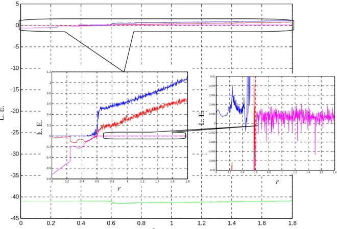
The Lyapunov exponents of the solutions of the nonlinear dynamical system, Eq. (1), are plotted in Fig. 1.

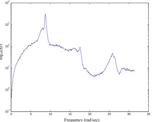
The three-dimensional projections of four dimensional phase portrait of the three positive Lyapunov exponents of new four dimensions the Chen system, Eq. (1), are plotted in Fig. 2. If the states are not periodic, their spectrum must be in terms of oscillations with a continuum of frequencies. Such a representation of the spectrum is called Fourier integral. The power spectrum analysis of the nonlinear dynamical system, Eq. (1), is shown in Fig. 3. The noise-like spectrum is characteristic of the chaotic dynamical system.

The divergence of flow Eq. (1) is defined by

1 2 3 4

29 0

a c b r r

x x x x

∂Π ∂Π ∂Π ∂Π

∇ ⋅Π = + + + = − + − + = − <

∂ ∂ ∂ ∂ , for 0≤ ≤

r

1.8, (3) where Π = & & & &

(

x x x x1, , ,2 3 4

)

. Therefore the three positive Lyapunov exponents of the new four dimensions Chen system is a forced dissipative system, which implies that the solution of the system, Eq. (1), is bounded as

t

→ ∞ .

Let

2 1

1 1 3 2 4

1 2 3

1 3 4

( ) 0

0 0

0 a x x

dx x x cx x x x bx

x x rx

− =

⎧⎪ − + − =

⎪⎨ − =

⎪⎪ + =

⎩

(4)

Solving the above equations, the three positive Lyapunov exponents of the new four dimensions Chen system yield five equilibrium points:

(6)

1

2 2

3 2

4

(0, 0, 0, 0)

( 1)( ) ( 1)( ) ( ) ( ) ( 1)( )

( , , , )

1 1 1 ( 1)

( 1)( ) ( 1)( ) ( ) ( ) ( 1)( )

( , , , )

1 1 1 ( 1)

( 1)( ) ( 1)( ) ( )

( , ,

1 1

EP

br r c d br r c d r c d c d br r c d

EP r r r r

br r c d br r c d r c d

EP r r r

− + − + + − + − +

− − − −

− + − + + + − +

− −

− − − −

− − + − − + +

− − ²

5 2

( ) ( 1)( )

, )

1 ( 1)

( 1)( ) ( 1)( ) ( ) ( ) ( 1)( )

( , , , )

1 1 1 ( 1)

c d br r c d r

EP r r r r

+ − − +

− − −

− − + − − + + + − − +

− −

− − − −

(5)

Substituting the constants a=35, b=6, c=12, d=7 and r=1.2 we obtain EP1(0, 0, 0, 0), EP2(26.15, 26.15, 114,

−2484.57), EP3(−26.15, −26.15, 114, 2484.57) , EP4(26.15i, 26.15i, 114, −2484.57i) and EP5(−26.15i,

−26.15i, 114, 2484.57i).

For EP1, the three positive Lyapunov exponents of the new four dimensions Chen system is linearized and the Jacobian matrix is defined as

1

.

0 0 35 35 0 0

0 1 7 12 0 1

0 0 0 0 0 6 0

0 0 0 0 0 0 1.2

a a

d c

J b

r

− −

⎡ ⎤ ⎡ ⎤

⎢ ⎥ ⎢ ⎥

= =

⎢ − ⎥ ⎢ − ⎥

⎢ ⎥ ⎢ ⎥

⎣ ⎦ ⎣ ⎦

(6)

The eigenvalues that correspond to EP1 are obtained as follows:

λ1＝−39.74, λ2＝16.74, λ3＝−6, λ4＝1.2

where λ1 and λ3 are two negative real numbers, and λ2 and λ4 are two positive real numbers. Therefore, the

EP

1 is a saddle point and unstable.

Next, linearizing the system about the non-zero equilibrium points EP2, EP3, EP4 and EP5 yields the following characteristic operation. Where the arbitrary point (x1, x2, x3, x4) has a Jacobian matrix equal to:

3 1

2

2 1

3 1 .

0 0

1 0 0

a a

d x c x

J x x b

x x r

⎡ − ⎤

⎢ − − ⎥

⎢ ⎥

=⎢ − ⎥

⎢ ⎥

⎣ ⎦

(7)

The eigenvalues that correspond to EP2 and EP3 are obtained as follows:

λ1＝1.2, λ2,3＝−5.9±62.52i, λ4＝−17.2

where λ1 is a positive real number, λ4 is a negative real number, and λ2 and λ3 are two imaginary roots with negative real parts. Therefore, EP2 and EP3 are saddle-foci points and unstable.

The eigenvalues that correspond to EP4 and EP5 are obtained as follows:

λ1＝9.18, λ2,3＝−19.48±52.74i, λ4＝19.78

where λ1 and λ4 are positive real numbers, and λ2 and λ3 are two imaginary roots with negative real parts.

Therefore, EP4 and EP5 are saddle-foci points and unstable.

The above brief analysis show that the five equilibrium points of the three positive Lyapunov exponents of the new four dimensions Chen system are all unstable.

(7)

3. Chaos Control Scheme by Adaptive Control

Consider the original chaotic or nonchaotic system

( , )ˆ ( )

x

&=

f x A

+

u t

(8) where

x

=

[ x x

1, , ,2 L

x

_n

]

^T∈

R

ⁿ denotes a state vector, Â is a vector of estimated parameters in f, f is a function vector, and

u t

( )=

[ u t u t

1( ), ( ), , ( )2 L

u t

_n

]

^T∈

R

ⁿ is a control input vector.

The goal system which can be either chaotic or nonchaotic, is

y g y B

& = ( , )ˆ (9) where

y

=

[ y y

1, , ,2 L

y

_n

]

^T∈

R

ⁿdenotes a state vector, ˆB is an estimated parameter vector, and g is a function vector. Our goal is to design an adaptive control method and a controller u(t) so that the state vector of the chaotic system (8) asymptotically approaches the state vector of the goal system (9).

The chaos control was achieved in that the limit of the error vector

e t

( )=

[ e e

1, ,2 L,

e

_n

]

^T approached zero:

lim 0

t

e

→∞ = (10) where

e y x

= − . (11) From Eq. (11),

e y x

& & & (12) = − ˆ

( , )ˆ ( , ) ( )

e g y B

&= −

f x A

−

u t

. (13) A Lyapnuov function ( , , )

V e A B

% % was chosen as a positive definite function:

1 1 1

( , , )

2 2 2

T T T

V e A B

% % =

e e

+

A A

% %+

B B

% % (14) where

A A A

% = − ˆ,

B B B

%= − ˆ, and ˆA , ˆB were the given parameters and A, B were the goal parameters.

The derivative along any solution of Eq. (13) and parameter dynamics was ˆ

( , , ) ^T[ ( , )ˆ ( , ) ( )]

V e A B

& ^% % =

e g y B

−

f x A

−

u t

+

AA BB

^{% %}^&+ % %^& (15) where u(t), A^&% and B&% were chosen so that V& =e C e A C A B C B^T ₁ + %^T ₂ %+ %^T ₃% , C1, C2 and C3 are diagonal negative definite matrices, and V& is a negative definite function of e, A% and B^%. In the current scheme of adaptive control of chaotic motion [30-32], traditional Lyapunov stability theorem and Babalat lemma were used to prove that as time approaches infinity, the error vector approached zero. However, the question remains as to why the estimated or also approaches uncertain or goal parameters.

4. Numerical Results of Chaos control

(8)

The goal system was a double harmonic system:

1 2 2 1 1

3 4 4 2 3

, ˆ ,

y y y y

ω ω

= = −

⎧⎨ = = −

⎩

& &

& & (16) where

ω

ˆ₁ and

ω

ˆ₂ were given constant parameters of the system with initial conditions y1(0)＝−0.7, y2(0)

＝0.3, y3(0)＝−0.4 and y4(0)＝0.8.

In order to lead (x1, x2, x3, x4) into (y1, y2, y3, y4), we added u1, u2, u3 and u4 to each equation in Eq. (1), respectively.

1 2 1 1 2 1 1 3 2 4 2

3 1 2 3 3 4 1 3 4 4

ˆ( ) , ˆ ˆ ,

ˆ , ˆ ,

x a x x u x dx x x cx x u

x x x bx u x x x rx u

⎧ = − + = − + − +

⎪⎨

= − + = + +

⎪⎩

& &

& & (17) where

a b c d

ˆ, , ,ˆ ˆ ˆ and

r were given constant parameters of the system with initial conditions x

ˆ 1(0)=0.5,

x

2(0)=−0.6, x3(0)=0.1 and x4(0)=−0.4. When the given parameters were

a

ˆ 35,=

b

ˆ= 6, ˆ 12, ˆ 7 and ˆ 0.97

c

=

d

=

r

= , the three positive Lyapunov exponents of the new four dimensions Chen system, are as shown in Fig. 1 and Fig. 2.

Subtracting Eq. (17) from the four equations in Eq. (16), we obtained the error dynamics in which the given parameters were

ω ω

^ˆ₁= ^ˆ₂ =0, aˆ=35, b^ˆ=6, cˆ=12, d^ˆ=7 and rˆ=1.2.

lim _i lim( _i _i) 0, 1, 2, 3, 4

t

e

t

y x i

→∞ = →∞ − = = (18)

1 2 2 1 1

2 1 1 1 1 3 2 4 2

3 4 1 2 3 3

4 2 3 1 3 4 4

ˆ( )

ˆ ˆ ˆ

ˆ ˆ

e y a x x u

e y dx x x cx x u

e y x x bx u

e y x x rx u

ω

= − − −

= − − + − + −

= − + −

= − − − −

&

(19)

where e1=y1−x1, e2= y2−x2, e3= y3−x3 and e4= y4−x4.

Choosing a Lyapunov function in the form of a positive definite function:

2 2 2 2 2 2 2 2 2 2 2

1 2 3 4 1 2 1 2 3 4 1 2

( , , , , , , , , , , ) 1( )

V e e e e a b c d r

% % % % %

ω ω

% % = 2

e

+ + + +

e e e a

% +

b

% +

c

% +

d

% +

r

% +

ω

% +

ω

%

(20)

where a a a%= − ˆ , b b b%= − ^ˆ , c c c%= −ˆ , d% = −d d^ˆ ,

r r r

%= −ˆ ,

ω ω ω

_%₁= ₁− ˆ₁ and

ω

_%₂ =

ω ω

₂ − ˆ₂ . The

1 2

ˆ ˆ ˆ ˆ

ˆ, , , , ,ˆ ˆ and

a b c d r

ω ω

were the given parameters, a=b=c=d=r=0, and ω1=ω2=1 were the goal parameters.

The time derivative along any solution of Eq. (19) and parameter dynamics was

1 2 2 1 1 2 1 1 1 1 3 2 4 2 3 4 1 2 3 3

4 2 3 1 3 4 4 1 1 2 2

ˆ ˆ

ˆ

ˆ ˆ

[ ( ) ] [ ] [ ]

ˆ ˆ

ˆ ˆ ˆ ˆ ˆ ˆ ˆ

[ ] ( ) ( ) ( ) ( ) ( ) ( ) ( )

V e y a x x u e y dx x x cx x u e y x x bx u

e y x x rx u a a b b c c d d r r

ω

ω ω ω ω ω

= − − − + − − + − + − + − + −

+ − − − − + − + − + − + − + − + − + −

&

& & & &

& % & % & % %

% % % (21)

(9)

Choosing

1 2 2 1 1 1

2 1 1 1 1 3 2 4 2 2

3 4 1 2 3 3 3

4 2 3 1 3 4 4 4

( )

u y a x x k e

u y dx x x cx x k e

u y x x bx k e

u y x x rx k e

ω

= − − +

= − − + − + +

= − + +

= − − − +

(22)

2 1 1 5 3 3 6

2 2 7 1 2 8

4 4 9

1 1 1 2 10 1 2 2 2 4 11 2

ˆ ( ) , ˆ ,

ˆ , ˆ ,

ˆ ,

ˆ , ˆ .

a a x x e k a b b e x k b

c c x e k c d d x e k d

r r x e k d

y e k y e k

ω ω ω ω ω ω

= − = − − − = − = −

= − = − − = − = − −

= − = − −

= − = − = − = −

&

& % %

&% %

&

& % %

&% %

& %

&%

& &

% % % %

(23)

Eq.(21) was the parameter dynamics. Substituting Eq. (22) and Eq. (23) into Eq. (21), we obtained

2 2 2 2 2 2 2 2 2 2 2

1 1 2 2 3 3 4 4 5 6 7 8 9 10 1 11 2

( ) 0

V& = − k e +k e +k e +k e +k a% +k b% +k c% +k d% +k r% +k

ω

% +k

ω

% <

which was a negative definite function of e1, e2, e3, e4, a b c d r%, , , , ,% % % %

ω

%₁ and

ω

%₂. The k1, k2, k3, k4, k5, k6, k7,

k

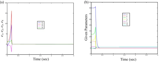
8, k9, k10 and k11 are positive feedback gains. Therefore, the Lyapunov asymptotical stability theorem was satisfied. The gains chose k1=197, k2=185, k3=149, k4=159, k5=30, k6=98, k7=145, k8=184, k9=127, k10=290 and k11=230. The obtained common origin of error dynamics (22) and parameter dynamics (23) were asymptotically stable. This means that the chaos control for different systems, from the three positive Lyapunov exponents of the new four dimensions Chen system to a double harmonic system, can be achieved.

The simulation results are shown in Fig. 4 and Fig. 5.

5. Chaotic Projective Hybrid Synchronization with Time Delay

We take the three positive Lyapunov exponents of new four dimensions Chen system given by (1) as the driving system, and the slave system with an adaptive control scheme which given by

1 2 1 1

2 1 1 3 2 4 2

3 1 2 3 3

4 1 3 4 4

( )

y a y y u

y dy y y cy y u y y y by u

y y y ry u

= − +

⎧⎪ = − + − +

⎪⎨ = − +

⎪⎪ = + +

⎩

&

(24)

where ui (i=1, …, 4) are the nonlinear controllers with initial conditions x1(0)＝0.5, x2(0)＝−0.6, x3(0)＝0.1,

x

4(0)＝−0.4, y1(0)＝−0.7, y2(0)＝0.3, y3(0)＝−0.4, and y4(0)＝0.8.

The system (1) and (24) is said to be in chaotic projective hybrid synchronization with time delay, if there exists a chaotic function z(t), such that

lim ( ) ( ) ( ) 0

t y t z t x t

τ

→∞ ± − = . (25) where ei(t) = yi(t)–zi(t)xi(t–τ), (

i

=1, 3), ei(t) = yi(t)+zi(t)xi(t–τ), (

i

=2, 4) and τ is delay time.

The chaotic projective function is a two-cell Quantum-CNN, the following differential equations are obtained [45]:

(10)

2

1 1 1 2

2 1 1 3 1 1 2 2

1 2

3 2 3 4

3

4 2 3 1 2 2 4

3

2 1 sin

( ) 2 cos

1

2 1 sin

( ) 2 cos

1

z z z

z z z z z

z

z z z

z z z z z

z α

ω α

α

ω α

⎧ = − −

⎪⎪ = − − +

⎪ −

⎪⎨

= − −

⎪⎪

⎪ = − − +

⎪ −

⎩

&

(26)

where z1, z3 are polarizations, z2, z4 are quantum phase displacements, α1 and α2 are proportional to the inter-dot energy inside each cell and ω1 and ω2 are parameters that weigh effects on the cell of the difference of the polarization of neighboring cells, like the cloning templates in traditional CNNs. Let α1＝19, α2＝13,

ω

1＝9, ω2＝7, z1(0)=−0.9, z2(0)=0.8, z3(0)=0.5, and z4(0)=−0.2.

Theorem. For the given chaotic function z(t), the chaotic projective hybrid synchronization between master system with time delay (1) and slave system

(24)

can be occurred using the following adaptive control method:

( )

2

1 1 1 2 1 1 1

1

2 1 3 1 3 1 1 2 2 2 2 1 3 2 2

1 2

3 1 2 2 3 4 3 3 1 2 3 3

4 1 3 2 1 3 2 3 2 4 4

3

2 1 sin ( )

( ) 2 cos ( ) ( ) ( )

1

2 1 sin ( ) ( ) ( )

( ) 2 cos ( )

1

u z z x t k e

u y y z z z z x t z x t x t k e

z

u y y z z x t z x t x t k e

u y y z z z z x t

z

α τ

ω α τ τ τ

α τ τ τ

ω α τ

= − − − +

⎛ ⎞

⎜ ⎟

= − − + − + − − +

⎜ − ⎟

⎝ ⎠

= − − − − + − − +

⎛ ⎞

⎜ ⎟

= − − − + − −

⎜ − ⎟

⎝ ⎠ ^{4 1} ³ ^{4 4}

2

( ) ( )

; 1, , 4

i i i

z x t x t k e

k g e i

τ τ

⎧⎪

⎪⎪

⎪⎪⎨

⎪⎪

⎪ − − +

⎪⎪

⎪ = − =

⎪⎩& L

(27)

where gi > 0 and τ=0.5 sec.

Proof. Define the chaotic projective hybrid synchronization with time delay error signal as e(t) = y(t)±z(t)x(t–τ), and yielding the following error dynamical system from Eq. (1) to Eq. (24)

( ) ^[ ^]

[ ]

( )

2

1 2 1 1 1 1 2 1 1 2 1

1

2 1 1 3 2 4 2 1 3 1 1 2 2 2

1

2 1 1 3 2 4

2

3 1 2 3 3 2 3 4 3 3

( ) 2 1 sin ( ) ( ) ( )

( ) 2 cos ( )

1

( ) ( ) ( ) ( ) ( )

2 1 sin ( )

e a y y u z z x t z a x t x t

e dy y y cy y u z z z z x t

z

z dx t x t x t cx t x t

e y y by u z z x t z

α τ τ τ

ω α τ

τ τ τ τ τ

α τ

= − + + − − − − − −

⎛ ⎞

⎜ ⎟

= − + − + + − + −

⎜ − ⎟

⎝ ⎠

+ − − − − + − − −

= − + + − − −

&

[ ]

1 2 3

3

4 1 3 4 4 2 1 3 2 2 4 4

3

4 1 3 4

( ) ( ) ( )

( ) 2 cos ( )

1

( ) ( ) ( )

x t x t bx t

e y y ry u z z z z x t

z z x t x t rx t

τ τ τ

ω α τ

τ τ τ

⎧⎪

⎪⎪

⎨⎪ − − − −

⎪⎪ ⎛ ⎞

⎪ = + + +⎜ − + ⎟ −

⎪ ⎜⎝ − ⎟⎠

⎪⎪ + − − + −

⎩

&

(28)

For the error dynamical system (28), we construct the following Lyapunov function:

(11)

( )

²

1 1

2 2

V e e

T

k l

= +

g

+

(29)

where l > 0 to be determined. Calculating the derivative of (29) along the trajectories of the error system (28), we have

( )

( ) ^[ ^]

{ }

[ ] }

2

1 2 1 1 1 1 2 1 1 2 1

1

2 1 1 3 2 4 2 1 3 1 1 2 2 2

1

2 1 1 3 2 4

2

3 1 2 3 3 2 3

1

( ) 2 1 sin ( ) ( )

( ) 2 cos ( )

1

( ) ( ) ( ) ( ) ( )

2 1 si

V e eT k l k g

e a y y u z z x z a x t x t

e dy y y cy y u z z z z x t

z

z dx t x t x t cx t x t

e y y by u z

α τ τ

ω α τ

τ τ τ τ τ

α

= − +

= − + + − − − − − +

⎧ ⎛ ⎞

⎪ − + − + +⎜ − + ⎟ −

⎨ ⎜ − ⎟

⎪ ⎝ ⎠

⎩

+ − − − − + − − −

+ − + + −

&

& &

&

( ) ^[ ^]

{ }

[ ] } ( )

( ) ( )

4 3 3 1 2 3

3

4 1 3 4 4 2 1 3 2 2 4 4

3

4 2

4 1 3 4

1

2 2 4 2

1 2 1 2 1 2 4 3 4

1

n ( ) ( ) ( ) ( )

( ) 2 cos ( )

1

( ) ( ) ( ) _i _i

i

i i

z x t z x t x t bx t

e y y ry u z z z z x t

z

z x t x t rx t k l e

e ae ae e de ce e be re le

τ τ τ τ

ω α τ

τ τ τ

=

− − − − − −

⎧ ⎛ ⎞

⎪ ⎜ ⎟

+ ⎨⎪⎩ + + +⎜⎝ − + − ⎟⎠ −

+ − − + − − +

= − + + − − + −

∑

0 0

2 0 1

2 2

0 0 0

0 1 0

2

T T

a d a

d a c

e lI e e Qe

b r

⎛⎡ − − ⎤ ⎞

⎜⎢ ⎥ ⎟

− −

⎜⎢ ⎥ ⎟

= −

⎜⎢ − ⎥ ⎟

⎜⎢ ⎥ ⎟

⎜⎢ − ⎥ ⎟

⎜⎢⎣ ⎥⎦ ⎟

⎝ ⎠

where I is the identity matrix. The l can be properly chosen to make the symmetry matrix Q is negative definite, and

( )

2 1, , 4

V

&≤ −

e

i

= L

. (30)

It is obvious that

V

& =0 if and only if ei(t) = 0,

(

ⁱ= L^1, ^{, 4}

)

, that is, the set

{ ( )

^, ²ⁿ^: ^0, ⁰ ⁿ

}

E

=

e k

∈

R e

=

k k

= ∈

R

is the largest invariant set contained in

^M

⁼

{ ^V

^& ⁼⁰

}

for system (28).

According to the well known LaSalle’s invariance principle, we have ei(t) = yi(t)–zi(t)xi(t–τ)→0, (

i

=1, 3), ei(t)

= yi(t)+zi(t)xi(t–τ)→0, (

i

=2, 4) and ki→k0i , ( 1, , 4)

i

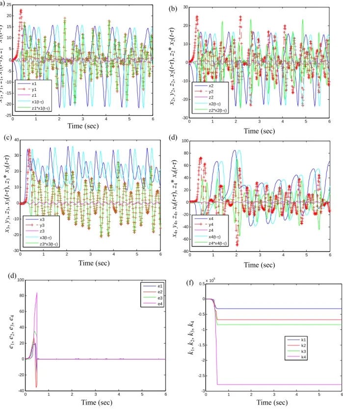
= L as t→∞. This completes the proof.

From the simulation results of Fig. 6, it is shown that chaotic function projective master system and slave system reach the synchronization state after they are controlled by the adaptive control. It is noticed that the synchronization effect is good.

(12)

6. Conclusions

In summary, the three positive Lyapunov exponents of the new four dimensions Chen system were investigated. Specifically, the adaptive control method for controlling chaos in different systems was studied.

It was found that where as traditional chaos control was limited in these systems, the proposed method had expanded chaos control functions. Based on Lyapunov stability theory and LaSalle’s invariance principle, we have designed the adaptive synchronization controllers to synchronize the two three positive Lyapunov exponents of the new four dimensions Chen systems. The theoretical result is verified by simulations to illustrate the effectiveness of the proposed adaptive chaotic function projective hybrid synchronization schemes.

References

[1] E. Ott, C. Grebogi, J.-A. Yorke, ‘‘Controlling chaos’’, Phys Rev Lett, 64, (1990), pp.1196-9.

[2] A.S. Elwakil and A.M. Soliman, ‘‘A family of Wien-type oscillators modified for chaos’’, Int. J. Circuit Theory & Applications, 25, (1997), pp.561-579.

[3] A.S. Elwakil and M.P. Kennedy, ‘‘High frequency Wien-type chaotic oscillator’’, Electronics Letters, 34, (1998), pp.1161-1162.

[4] Z.-M. Ge and C.-H. Yang, “Pragmatical generalized synchronization of chaotic systems with uncertain parameters by adaptive control”, Physica D: Nonlinear Phenomena, 231, (2007), pp.87-94.

[5] Z.-M. Ge and C.-H. Yang, “The generalized synchronization of a Quantum-CNN chaotic oscillator with different order systems”, Chaos, Solitons, and Fractals, 35, (2008), pp.980-990.

[6] Z.-M. Ge and, C.-M. Chang, ‘‘Chaos Synchronization and Parameters Identification of Single Time Scale Brushless DC Motors, Chaos’’, Solitons and Fractals, 20, (2004), pp.883-903.

[7] Z.-M. Ge and C.-H. Yang, “The symplectic synchronization of different chaotic systems”, , Chaos, Solitons, and Fractals, 40, (2009), pp.2532-2543.

[8] Z.-M. Ge and W.-Y. Leu, ‘‘Chaos Synchronization and Parameter Identification for Identical System’’, Chaos, Solitons and Fractals, 21, (2004), pp.1231-1247.

[9] Z.-M. Ge and C.-H. Yang, “Synchronization of complex chaotic systems in series expansion form”, Chaos, Solitons, and Fractals, 34, (2007), pp.1649-58.

[10] Z.-M. Ge and Y.-S. Chen, ‘‘Synchronization of Unidirectional Coupled Chaotic Systems via Partial Stability’’, Chaos, Solitons and Fractals, 21, (2004), pp.101-111.

[11] Z.-M. Ge, C.-H. Yang , H.-H. Chen and S.-C. Lee, ‘‘Non-linear dynamics and chaos control of a physical pendulum with vibrating and rotation support’’, Journal of Sound and Vibration, 242, (2001), pp.247-264.

[12] H. Haken, Physics Letters A, 1983, (94), 71.

[13] S. Hayes, C. Gerbogi, E. Ott, Physical Review Letters, 70, (1993), 3031.

[14] M.P. Kennedy, IEEE Trans. Circuits & Syst.-I, 41, (1994), 771.

[15] E. Lindberg, A. Tamasevicius, A. Cenys, G. Mykolaitis, A. Namajunas, Hyperchaos via X-Diode, Proceedings of the 6th international specialist workshop on nonlinear dynamics of electronic systems, Budapest, (1998), pp.125-128.

[16] T. Matsumoto, L.O. Chua, K. Kobayashi, IEEE Trans. Circuits & Syst.-I, 33, (1986), 1143.

[17] A. Namajunas, A. Tamasevicius, Electronics Letters, 32, (1996), 945.

[18] A. Namajunas, K. Pyragas, A. Tamasevicius, Physics Letters A, 201, (1995), 42.

(13)

[19] R.W. Newcomb, S. Sathyan, IEEE Trans. Circuits & Syst.-I, 30, (1983), 54.

[20] T.S. Parker, L.O. Chua, Practical numerical algorithms for chaotic systems, Springer, New York, 1989.

[21] A. Parlitz, T. Kocarev, H. Preckel, Physical Review E, 53, (1996), 4351.

[22] O.E. Rossler, Physics Letters A, 71, (1979), 155.

[23] T. Saito, IEICE Trans. Fundamentals, E75-A, (1992), 294.

[24] A. Tamasevicius, A. Namajunas, A. Cenys, 32, (1996), 957.

[25] William Ott and James A. Yorke, Physical Review E 78, (2008), 056203.

[26] Z.-M. Ge and C.-H. Yang, Physics Letters A, 373, (2009), 349.

[27] G. Chen and X. Dong, From Chaos to Order, World Scientific, New Jersey, pp. 48, 1998.

[28] T.S. Kuhn, The Structure of Scientific Revolution, third edition, The University of Chicago Press, Chicago and London, pp.7, 1962, 1970, 1996.

[29] I.B. Cohen, Revolution in Science, Six printing, The Belknap Press of Harvard University Press, Cambridge, Massachusetts , pp.467, 1985, 1994 .

[30] J.-H. Park, Chaos, Solitons and Fractals, 26, (2005), 959.

[31] J.-H. Park, Chaos, Solitons and Fractals, 25, (2005), 333.

[32] E. M. Elabbasy, H. N. Agiza and, M. M. El-Desoky, Chaos, Solitons and Fractals, 30, (2006), 1133.

[33] G. Chen and X. Dong, From chaos to order: methodologies, perspectives and applications, Singapore:

World Scientific; 1998.

[34] G. Chen and X. Dong, IEEE Trans Circ Syst I, (1993), 591 . [35] G. Chen and X. Yu, IEEE Trans Circ Syst I; 46, (1999), 767.

[36] X. Guan, C. Chen, Z. Fan and H. Peng, Int J Bifurcat Chaos, (2003), 193.

[37] K. Keiji, H. Michio and K. Hideki, Phys Lett A, 245, (1998), 511.

[38] M. Jang, Int J Bifurcat Chaos, 12, (2002), 1437.

[39] C. Fuh and P. Tung, ,, Phys Lett A, 218, (1996), 240.

[40] X. Yu, Chaos, Solitons and Fractals, 8, (1997), 1577.

[41] Y. Yu and S. Zhang, Chaos, Solitons and Fractals, 15, (2003), 897.

[42] M. Bernardo, Phys Lett A, 214, (1996), 139.

[43] F. Moez, , Chaos, Solitons & Fractals, 15, (2003), 883.

[44] Y.-J. Cao, Phys Lett A, 270, (2000), 171.

[45] L.G. Fortuna, D. Porto, Int. J. Bifur. Chaos, 14, (2004), 1085.

[46] W. Yang and J. Sun, Physics Letters A, 374, (2010), 557

(14)

Fig. 1. Lyapunov exponents of the three positive Lyapunov exponents of new four dimensions Chen system, with a=35, b=6, c=12, d=7.

Fig. 2. The three-dimensional projections of four-dimensional phase portrait of the three positive Lyapunov exponents of new four dimensions Chen system, with a=35, b=6, c=12, d=7 and r=1.2.

-10 -5

0 5

10 15

20

-10 -5 0 5 10 15 20

0 5 10 15 20 25 30 35

x1

x2

x3

(a)

-20 -15 -10 -5 0 5 10 15 20

-10 -5 0 5 10 15 20 -40 -20 0 20 40 60

x1

x2

x4

(b)

-20 -15 -10 -5 0 5 10 15

20

0 10 20 30 40 50 -40 -20 0 20 40 60

x1

x3

x4

(c)

-15 -10 -5

0 5

10 15

20

10 20 30 40 50 60 -40 -20 0 20 40 60

x2

x3

x4

(d)

0 0.2 0.4 0.6 0.8 1 1.2 1.4 1.6 1.8

-45 -40 -35 -30 -25 -20 -15 -10 -5 0 5

r r r

L. E.

0 0.2 0.4 0.6 0.8 1 1.2 1.4 1.6 1.8

-0.8 -0.6 -0.4 -0.2 0 0.2 0.4 0.6 0.8 1 1.2

L. E.

0 0.2 0.4 0.6 0.8 1 1.2 1.4 1.6 1.8

-0.01 -0.008 -0.006 -0.004 -0.002 0 0.002 0.004 0.006 0.008 0.01

L. E.

(15)

Fig. 3. Power spectrum of y for three positive Lyapunov exponents of new four dimensions Chen system, with

a=35, b=6, c=12, d=7 and r=1.2.

Fig. 4. The three-dimensional projections of four-dimensional phase portrait of a double harmonic system.

0 5 10 15 20 25 30 35

10^-1 10⁰ 10¹ 10² 10³ 10⁴

Frequency (rad/sec) log10(Sy)

-0.8 -0.6 -0.4 -0.2 0 0.2

0.4 0.6 0.8

-1 -0.5 0 0.5 1 -1 -0.5 0 0.5 1

y1

y2

y3

(a)

-0.8 -0.6 -0.4 -0.2 0 0.2 0.4 0.6

0.8

-1 -0.5 0 0.5 1 -1 -0.5 0 0.5 1

y1

y2

y4

(b)

-0.8 -0.6 -0.4 -0.2 0 0.2 0.4 0.6

0.8

-1 -0.5 0 0.5 1 -1 -0.5 0 0.5 1

y1

y3

y4

(c)

-0.8

-0.6 -0.4 -0.2 0 0.2 0.4 0.6

0.8

-1 -0.5 0 0.5 1 -1 -0.5 0 0.5 1

y2

y3

y4

(d)

(16)

Fig. 5. Time histories of state errors, a b c d rˆ, , , , ,^ˆ ˆ ^ˆ ˆ ωˆ₁ and ω . ˆ₂ Time (sec)

e1, e2, e3, e4

(a)

0 0.5 1 1.5 2 2.5 3

-5 0 5 10 15 20

e1 e2 e3 e4

0 0.5 1 1.5 2 2.5 3

-5 0 5 10 15 20 25 30 35 40

a b c d r w1 w2

Time (sec)

Given Parameters

1 2

ˆˆ ˆˆ ˆˆ ˆ a bc dr ωω

(b)

(17)

Fig. 6. Time histories of state errors, k1, k2, k3, and k4.

0 1 2 3 4 5 6

-30 -20 -10 0 10 20 30 40

x3 y3 z3 x3(t-τ) z3*x3(t-τ)

Time (sec) x3, y3, z3, x3(t-τ), z3* x3(t-τ)

(c)

0 1 2 3 4 5 6

-80 -60 -40 -20 0 20 40 60 80 100

x4 y4 z4 x4(t-τ) z4*x4(t-τ)

(d)

0 1 2 3 4 5 6

-30 -20 -10 0 10 20 30

x2 y2 z2 x2(t-τ) z2*x2(t-τ)

(b)

0 1 2 3 4 5 6

-25 -20 -15 -10 -5 0 5 10 15 20 25

x1 y1 z1 x1(t-τ) z1*x1(t-τ)

(a)

0 1 2 3 4 5 6

-3 -2.5 -2 -1.5 -1 -0.5 0 0.5x 10⁵

k1 k2 k3 k4

Time (sec) (f)

k1, k2, k3, k4

0 1 2 3 4 5 6

-40 -20 0 20 40 60 80 100

e1 e2 e3 e4

Time (sec) (d)

e1, e2, e3, e4

(18)

無研發成果推廣資料

(19)

98 年度專題研究計畫研究成果彙整表

計畫主持人：楊振雄計畫編號：98-2218-E-011-010-

計畫名稱：具有三個正的 Lyapunov 指數新四階 Chen 系統之超渾沌、渾沌控制與同步研究量化

成果項目 ^{實際已達成}

數（被接受或已發表）

預期總達成數(含實際已

達成數)

本計畫實際貢獻百

分比

單位

備註（質化說明：如數個計畫共同成果、成果列為該期刊之封面故事 ...

等）

期刊論文 0 0 0%

研究報告/技術報告 0 0 0%

研討會論文 0 0 0%

論文著作篇

專書 0 0 0%

申請中件數 0 0 0%

專利已獲得件數 0 0 0% 件

件數 0 0 0% 件

技術移轉

權利金 0 0 0% 千元

碩士生 1 1 100%

博士生 1 1 100%

博士後研究員 0 0 0%

國內

參與計畫人力

（本國籍）

專任助理 0 0 0%

人次

期刊論文 0 2 0%

研究報告/技術報告 0 0 0%

研討會論文 0 0 0%

論文著作篇

專書 0 0 0% 章/本

申請中件數 0 0 0%

專利已獲得件數 0 0 0% 件

件數 0 0 0% 件

技術移轉

權利金 0 0 0% 千元

碩士生 0 0 0%

博士生 0 0 0%

博士後研究員 0 0 0%

國外

參與計畫人力

（外國籍）

專任助理 0 0 0%

人次

(20)

其他成果

(

無法以量化表達之成

果如辦理學術活動、獲得獎項、重要國際合作、研究成果國際影響力及其他協助產業技術發展之具體效益事項等，請以文字敘述填列。)

無

成果項目量化 名稱或內容性質簡述

測驗工具(含質性與量性) 0

課程/模組 0

電腦及網路系統或工具 0

教材 0

舉辦之活動/競賽 0

研討會/工作坊 0

電子報、網站 0

科教處計畫加填項

目計畫成果推廣之參與（閱聽）人數 0

(21)

(22)

國科會補助專題研究計畫成果報告自評表

請就研究內容與原計畫相符程度、達成預期目標情況、研究成果之學術或應用價值（簡要敘述成果所代表之意義、價值、影響或進一步發展之可能性）、是否適合在學術期刊發表或申請專利、主要發現或其他有關價值等，作一綜合評估。

1. 請就研究內容與原計畫相符程度、達成預期目標情況作一綜合評估

□達成目標

■未達成目標（請說明，以 100 字為限）

□實驗失敗

□因故實驗中斷

■其他原因說明：

因計畫為 24 個月的時間,但核定為 11 個月, 故執行約 1/3~1/2 計畫

2. 研究成果在學術期刊發表或申請專利等情形：

論文：□已發表 □未發表之文稿 ■撰寫中 □無專利：□已獲得 □申請中 ■無

技轉：□已技轉 □洽談中 ■無其他：（以 100 字為限）

3. 請依學術成就、技術創新、社會影響等方面，評估研究成果之學術或應用價值（簡要敘述成果所代表之意義、價值、影響或進一步發展之可能性）（以 500 字為限）

本計畫發現 4 階的 Chen 系統有 3 個正李雅普夫指數,渾沌控制與渾沌同步均達到預期結果

具有三個正的Lyapunov指數新四階Chen系統之超渾沌、渾沌控制與同步研究

行政院國家科學委員會專題研究計畫 成果報告

具有三個正的 Lyapunov 指數新四階 Chen 系統之超渾沌、

渾沌控制與同步研究 研究成果報告(精簡版)

中 華 民 國 99 年 09 月 29 日

行政院國家科學委員會補助專題研究計畫 ■成果報告

□期中進度報告

具有三個正的 Lyapunov 指數新四階 Chen 系統之超渾沌、渾沌控制 與同步研究

計畫類別：■個別型計畫 □整合型計畫 計畫編號：NSC 98－2218－E－011－010－

執行期間： 98 年 9 月 1 日至 99 年 7 月 31 日 執行機構及系所：國立臺灣科技大學/自動化及控制研究所

計畫主持人：楊振雄 共同主持人：

計畫參與人員：呂紹安、武光輝

成果報告類型(依經費核定清單規定繳交)：■精簡報告 □完整報告

本計畫除繳交成果報告外，另須繳交以下出國心得報告：

□赴國外出差或研習心得報告

□赴大陸地區出差或研習心得報告

□出席國際學術會議心得報告

□國際合作研究計畫國外研究報告

處理方式：除列管計畫及下列情形者外，得立即公開查詢

□涉及專利或其他智慧財產權，□一年■二年後可公開查詢 中 華 民 國 年 月 日

國科會補助專題研究計畫成果報告自評表

1. 請就研究內容與原計畫相符程度、達成預期目標情況作一綜合評估

□ 達成目標

■ 未達成目標（請說明，以 100 字為限）

□ 實驗失敗

□ 因故實驗中斷

■ 其他原因

說明：因計畫為 24 個月的時間,但核定為 11 個月, 故執行約 1/3~1/2 計畫

2. 研究成果在學術期刊發表或申請專利等情形：

論文：□已發表 □未發表之文稿 ■ 撰寫中 □無 專利：□已獲得 □申請中 ■ 無

技轉：□已技轉 □洽談中 ■ 無 其他：（以 100 字為限）

3. 請依學術成就、技術創新、社會影響等方面，評估研究成果之學術或應用價 值（簡要敘述成果所代表之意義、價值、影響或進一步發展之可能性）（以 500 字為限）

本計畫發現 4 階的 Chen 系統有 3 個正李雅普夫指數,渾沌控制與渾沌同 步均達到預期結果

Abstract

1. Introduction

2. Three Positive Lyapunov Exponents of New Four Dimensions Chen System and its Equilibrium

a c b r r

x x x x

r

(

)

t

Let

a a

d c

J b

r

EP

3. Chaos Control Scheme by Adaptive Control

x

f x A

u t

x

[ x x

x

]

R

u t

[ u t u t

u t

]

R

y g y B

y

[ y y

y

]

R

e t

[ e e

e

]

e

e y x

e y x

e g y B

f x A

u t

V e A B

V e A B

行政院國家科學委員會專題研究計畫成果報告

渾沌控制與同步研究研究成果報告(精簡版)

中華民國 99 年 09 月 29 日

具有三個正的 Lyapunov 指數新四階 Chen 系統之超渾沌、渾沌控制與同步研究

計畫類別：■個別型計畫 □整合型計畫計畫編號：NSC 98－2218－E－011－010－

執行期間： 98 年 9 月 1 日至 99 年 7 月 31 日執行機構及系所：國立臺灣科技大學/自動化及控制研究所

計畫主持人：楊振雄共同主持人：

□涉及專利或其他智慧財產權，□一年■二年後可公開查詢中華民國年月日

論文：□已發表 □未發表之文稿 ■ 撰寫中 □無專利：□已獲得 □申請中 ■ 無

技轉：□已技轉 □洽談中 ■ 無其他：（以 100 字為限）

3. 請依學術成就、技術創新、社會影響等方面，評估研究成果之學術或應用價值（簡要敘述成果所代表之意義、價值、影響或進一步發展之可能性）（以 500 字為限）

本計畫發現 4 階的 Chen 系統有 3 個正李雅普夫指數,渾沌控制與渾沌同步均達到預期結果