應用真實流向概念重建通量法則於靜直接模擬法速解尤拉方程式的研究

國

立

交

通

大

學

機 械 工 程 學 系

博 士 論 文

應用真實流向概念重建通量法則於靜直接模擬法速解尤拉方

程式的研究

Development of Volume-to-Volume True-Direction Flux

Reconstruction Scheme in the Quiet Direct Simulation Method for

Euler Equation

研 究 生：林雅茹

指導教授：吳宗信 博士

應用真實流向概念重建通量法則於靜直接模擬法速解尤拉方

程式的研究

Development of Volume-to-Volume True-Direction Flux

Reconstruction Scheme in the Quiet Direct Simulation Method for

Euler Equation

學生: 林雅茹

Student : Ya-Ju Lin

指導教授: 吳宗信 博士

Advisor : Dr. Jong-Shinn Wu

國 立 交 通 大 學

機 械 工 程 學 系

博

士

論

文

A Thesis

Submitted to Institute of Mechanical Engineering Collage of

National Chiao Tung University

In Partial Fulfillment of the Requirements

for the Degree of

Doctor of Philosophy

in

Mechanical Engineering

July 2013

Hsinchu, Taiwan

西 元

2 0 1 3 年 7 月

應用真實流向概念重建通量法則於靜直接模擬法速解尤

拉方程式的研究

學生: 林雅茹

指導教授: 吳宗信 博士

國立交通大學

機械工程學系博士班

中文摘要

近年來一項以模擬粒子為基礎來解非黏滯尤拉方程式的數值方法稱之為靜態 直接模擬法（Quiet Direct Simulation, QDS）[Albright et al., 2002]。此方法利用高

司 -赫麥（Gauss-Hermite）積分集合式來取代馬克斯威爾與波茲曼（Maxwell-Boltzmann）速度分佈的表示。不僅可以輕易地處理流體中急遽變化的變數分佈 （如大部分的計算流體力學一樣）更可以準確的仿效真實流的運行方式引入真實 方向的守恒場，又因為具有地域性高（不需要大範圍考慮周遭的網格）的特點使 得平行化的計算程式得以輕易達成。由於在每個網格內都擁有相同的離散速度分 佈，因此對於計算時所要求的記憶體需求可減至最低。但所謂有一利必有一弊， 因而衍生出數值擴散性（numerical diffusion）太強等問題，驅使 Smith 等人 [Smith et al., 2009]發展出另一項以近二階 QDS 方法（QDS-2N）來改善相關問題 以達到大幅提升數值的精確度。但是，在改善的過程中仍未真正考慮到流體真實 流向的概念而有所遺憾。為解決此問題，本論文將對此數值方法提出改善方法並 且用理論分析的角度進行探討。 在第一部份方面，就數值方法的觀點來說，本論文一樣是利用以近二階靜態 直接模擬法來求解尤拉方程式，目的是發展一項根據流體的真實流向概念而進行 的重建通量法則，我們稱之為 QDS-N2 法。不同於傳統的有限差分法是把通量計 算存取於網格間的界面，相較之下，QDS 則是根據流體的真實流向來決定該網格

全遵循流體真實流向之計算法。在計算通量之前，我們會在每一個網格中引入數 顆 QDS 粒子，而此粒子根據瞬間加權擁有守恒場的變數值，並包含了質量、動 量與能量等計算值。甚至守恒場的變數值變化情形（可以依據多項式表示）在同 一網格中皆可被允許隨空間變化。雖然在一維流流場中，QDS-N2 法的重建通量 表示式與 QDS-2N 法的重建通量表示式是一模一樣，不過在流場延伸至多維度時 兩種方法卻有所不同。為了呈現兩方法的優異性，在二維流的計算中，我們經由 幾項不同的算例結果來驗證此新的流量重建法的優異性，並且在第二部份理論分 析方面以解析解的方式探討與 QDS-2N 方法的差異。文中我們對於二維的研究比 對項目包含了震波撞擊低壓近似氣泡問題、尤拉四震波的交互作用問題、尤拉四 面波交互作用問題、三馬赫波正面衝擊水平台階和水平渦流擾動問題。並且對於 模擬時所耗費的計算時間與更高階計算之效果做進一步的探討。根據結果顯示， 在相較於 QDS-2N 法的情況之下，本文所提出的多維度重建法則在計算的精確度 上確實有很大的提升。以得到相同數值精確度的標準而言，屏除因考慮流體真實 流向而增加計算量所耗費的時間外，就水平渦流擾動問題的結果來說，相較於 QDS-2N 法，QDS-N2法在計算上所消耗的時間可以大幅減少。此外，誠如先前所 提及 QDS 乃是一個高地域性的數值方法，非常有利於分散式叢集電腦上進行平 行計算。因此，發展三維的 QDS 數值方法也將一併利用平行方式進行。而文中 所有提及平行效率的研究與相關的平行計算，皆在台灣國家實驗研究院所屬國家 高速網路與計算中心內所提供的 ALPS 叢集電腦中完成。就平行效率的研究方面， 我們在計算大尺度的問題時使用高達 256 顆處理器分別完成 0.5、2、12.5 百萬的 計算網格，根據 strong scaling 所得的結果顯示，得到的平行效率可達 75%、 68.5%與 65.5%。另一項 weak scaling 的研究，比對理想值為 1.0 的平行效率，使 用本方法所得到的效率可達 1.2，其中處理器最高達到 128 顆，而平均每一顆處 理器皆包含計算2 萬個計算網格。 在第二部份理論分析方面，我們將所有有關質量、動量與能量的通量分別對 QDS-2N 和 QDS-N2 兩種數值方法進行解析解的分析推導。比較方式是針對兩運 算法在流場中因不同變數值的改變於彼此之間所產生的通量差異。結果顯示二者 通量值於低密度、低溫與高速的流域範圍中較易產生較大差異，而此範圍往往也 是擴散波出現的地方。除此之外，本研究觀察到當兩數值方法在處理水平和垂直 軸（x 軸與 y 軸）的計算問題時彼此所產生的通量值差異甚小，反之在計算斜角

流場時會相差較大。因此，可以根據本研究結果知道在未來處理模擬流場等問題

時，得以輕易地判斷合適於問題的 QDS-N2法或 QDS-2N 方法而有效地取得所預

期的結果，高精確度以利分析或是快速地得到流場趨勢。 對於主要的研究結果與未來研究方向的建議將總結於文末。

Development of Volume-to-Volume True-Direction Flux

Reconstruction Scheme in the Quiet Direct Simulation

Method for Euler Equation

Student: Ya-Ju Lin Advisor: Dr. Jong-Shinn Wu

Department of Mechanical Engineering

National Chiao Tung University

Abstract

A particle-based quiet direct simulation (QDS) method [Albright et al., 2002] was invented to solve the inviscid Euler equation, in which the Maxwell-Boltzmann velocity distribution is enforced through the use of Gauss-Hermite quadrature integration without using any random number. It is a very fast Euler equation solver, which is deterministic with large dynamic range of flow properties like most conventional CFD methods, employs true-direction conservative fluxes for faithfully mimicking real flow motion, is highly localized (a small stencil) for easier parallelization and requires very low memory because the discrete velocities can be re-used in each cell. However, it is numerically very diffusive and has been extended to a nearly second-order numerical scheme by Smith et al. [2009] without really considering true-direction flux reconstruction. Thus, we intend to further address this problem from both numerical and theoretical viewpoints in this thesis.

In the numerical part, a true-direction flux reconstruction of the second-order quiet direct simulation (QDS) as an equivalent Euler equation solver, called QDS-N2_{, is}

(true direction) fluxes are computed, as opposed to fluxes at cell interfaces as employed by traditional finite volume schemes, a volumetric reconstruction is required to reach a totally true-direction scheme. The conserved quantities are permitted to vary (according to a polynomial expression) across all simulated dimensions. Prior to the flux computation, QDS particles are introduced using properties based on weighted moments taken over the polynomial reconstruction of the conserved variables such as mass, momentum and energy. The resulting flux expressions are shown to exactly reproduce the existing second-order extension for a one-dimensional flow, while providing a means for true multi-dimension reconstruction.The new reconstruction is demonstrated in several verification studies. These include several two-dimensional test cases such as shock bubble interaction problem, an Euler-four-shock interaction, Euler-four-contact interaction, Mach 3 facing over a forward step, and the advection of a vortical disturbance. These results are presented, and the increased computational time and the effect of higher-order extension are discussed. The results show that the proposed multi-dimensional reconstruction provides a significant increase in the accuracy of the solution as compared to the previously developed QDS-2N method. We show that, despite the increase in the computational expense, the computational speed of the proposed QDS-N2 method is several times higher than that of the previously proposed QDS-2N method for a fixed degree of numerical accuracy, at least, for the test problem of the advection of vertical disturbances. As mentioned earlier, QDS method is intrinsically a highly localized numerical scheme, which makes it highly suitable for parallel computing on distributed-memory cluster machines using domain decomposition. With parallel implementation, an extension to three-dimensional QDS method is also demonstrated. The results show that the parallel efficiency, based on a strong scaling study, for a large-scale problem using 0.5, 2, and 12.5 million cells can

reach up to 75%, 68.5%, and 65.5% with 256 processors respectively. In addition, the parallel efficiency, based on a weak scaling study, for a shock bubble interaction is 1.2, which the ideal efficiency is 1.0, up to 49 processors for 20,000 cells per processor. Note all the parallel performance tests were performed at the APLS cluster of National Center for High-Performance Computing, Taiwan.

In the theoretical part, we have derived the analytical expressions of all the fluxes related to mass, momentum and energy in the two-dimensional QDS-N2 and QDS-2N methods respectively. Comparisons are made systematically between the corresponding fluxes in the two methods by varying flow properties. Results show that a large discrepancy of fluxes between these two methods occurs in the ranges of low density, low temperature, and high velocity.It is also interesting to learn that this range of gas flow often corresponds to an expansion wave region. Moreover, the fluxes using both methods are similar horizontal and vertical directions (x and y-direction), while large discrepancy is found in the fluxes going to the diagonal direction.With this observation, we can evaluate the accuracy of QDS-2Nmethod as compared to QDS-N2 method in the flow field, which may be important in deciding which method to be used for different flow problems.

The major findings of the research with the recommendations for future study are summarized at the end of the thesis.

誌謝

本篇論文得以完成最要感謝的是指導教授 吳宗信老師的細心指導。感謝吳 老師在論文指導時所花的時間與精力，並且感謝口試委員陳慶耀老師、林昭安老 師、牛仰堯老師、黃俊誠老師與陳明志老師百忙中遠道而來並對於學生的研究成 果與論文撰寫上提供許多寶貴的意見與精闢的見解，使學生獲益良多讓論文得以 更加完整。在求學的過程中，感恩於老師的指導使得學生在學習上成長不少，讓 學生在學術研究上更加精益求精，在研究態度上變得更加嚴謹、敏銳，並且從老 師認真且專業的指導上見識到機械熱流領域是如此的深奧與廣泛。不僅如此，於 生活上，在老師的啟蒙下，學生不僅對於台灣國家環境的認知更加的多元，社會 脈動更加的關懷。由衷的感謝老師對於學生在研究的環境上提供國際化的思維， 並且讓學生在求學的道路上有機會出國至美國、日本參加國際會議體驗國際交流 所帶來的研究熱誠。 回首六年來在交大的求學歷程，特別要感謝李汶樺博士、Dr. Hadley Cave 與 捷燦學長在研究上耐心的指導與無私的協助使學生渡過無數學習的障礙，並感謝 孟華學姐一路來的相挺與陪伴得以撐過漫長的歲月。還要感謝實驗室學長昆模、 沅明、一同畢業的學弟正勤、總是默默付出的學弟古必任、瑞祥、子豪、冠榮、 熱心的明忠、仁寶、芳安、聖毅、文靜的垂青、世昕、易軒、哲偉、奇融、廷浩、 電漿實驗室的宜偉、至東、志華、俊平、國淳、光堯、學妹青榕，在實驗室的相 處中，不論是課業、研究或生活上都得到許多扶持。 最後僅將本論文獻給我摯愛的家人及許家偉先生一直以來對我的照顧並時時 刻刻的關懷、無怨尤的陪伴，因為你們殷切的期盼，讓我有上進的動力；因為你 們積極的鼓勵，讓我完成困難的學業。 林雅茹

Table of Contents

中文摘要 ... I  

Abstract ... IV  

誌謝 ... VII  

Table of Contents ... VIII  

List of Table ... X  

List of Figures ... XI  

Nomenclature ... XVIII  

Chapter 1   Introduction ... 1  

1.1 Background and Motivation ... 1  

1.1.1 Direct Simulation Monte Carlo Method ... 1  

1.1.2 Quiet Direction Simulation Monte Carlo Method ... 2  

1.2 Literature Survey ... 3  

1.3 Specific Objectives of this Thesis ... 6  

Chapter 2   Numerical Methods ... 8  

2.1 Overview of Euler Equation Solver ... 8  

2.1.1 Computational Fluid Dynamics ... 8  

2.1.2 Kinetic Method ... 9  

2.2 Quiet Direct Simulation (QDS) Method ... 11  

2.3 QDS-2N Method ... 15  

2.4 QDS-N2 Method ... 18  

2.4.1 Spatial Reconstruction and Flux Calculation ... 18  

2.4.2 One-Dimensional Flux Calculation and Implementation ... 21  

2.4.3 Two-Dimensional Flux Calculation and Implementation ... 22  

2.4.4 Three-Dimensional Flux Calculation and Implementation ... 24  

2.5 Brief Summary ... 25  

Chapter 3   Complex Gas Flow Simulations using the QDS-N2 Method ... 27  

3.1 Introduction ... 27  

3.2 QDS Method in One-Dimension Flow ... 27  

3.2.1 Shock Tube ... 27  

3.2.2 Shock-blast wave interaction ... 28  

3.2.3 Shock acoustic wave interaction ... 29  

3.3.1Shock-Bubble Interaction ... 30  

3.3.2 Euler-Four-Shocks problem ... 31  

3.3.3 Euler-Four-Contacts problem ... 32  

3.3.5 Shock Wave Diffraction over a 90 degree sharp corner ... 35  

3.3.6 Advection of Vortical Disturbance ... 37  

3.4 QDS Method in Three-Dimension Flow ... 39  

3.4.1 Mach 2 Flow over a Pillar ... 40  

3.5 Parallel Computing of QDS method ... 41  

3.5.1 Overview of Parallel Implementation ... 41  

3.5.2 Simulation Conditions ... 41  

3.5.3 Parallel Performance ... 42  

3.5.3.1 Weak Scaling ... 42  

3.5.3.2 Strong Scaling ... 43  

3.6 Brief Summary ... 44  

Chapter 4   Difference Analysis of 2NMethod as Compared to QDS-N2_{Method ... 46}  

4.1 Introduction ... 46  

4.2 Derivation of Analytical Fluxes of QDS Methods (2N vs. N2) ... 46  

4.2.1 Mass Flux ... 46  

4.2.2 Momentum Fluxes ... 48  

4.2.3 Energy Flux ... 49  

4.3 Results and Discussion ... 50  

4.3.1 Diagrams of Relative Difference Distribution ... 50  

4.3.2 Example with Large Difference ... 51  

4.3.2.1 Shock-Bubble Interaction ... 52  

4.3.2.2. Euler-Four-Shock Simulation ... 53  

4.3.2.3 Mach 3 Flow over a Forward Step ... 54  

4.3.2.4 Shock Wave Diffraction over a 90-degree Sharp Corner ... 55  

4.4 Brief Summary ... 56  

Chapter 5   Conclusion and Recommendations of Future Work ... 58  

5.1 Summary ... 58  

5.1.1 Numerical Investigation of QDS-N2 _{Method ... 58}  

5.1.2 Theoretical Analyses of Conservation Fluxes of 2N Method and QDS-N2 _{Method ... 59}  

5.2 Recommendations of Future Work ... 60  

References ... 61  

Appendix A ... 67  

List of Table

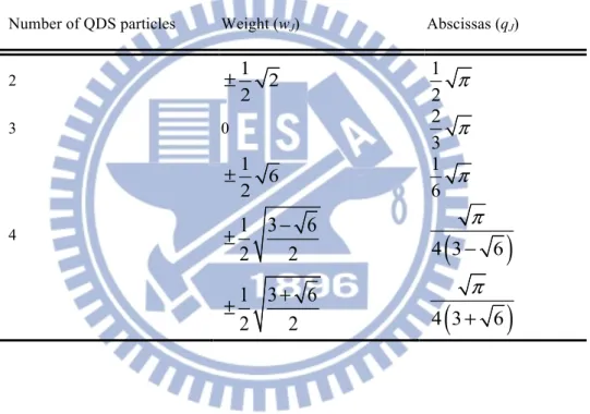
Table 2-1 The value of weight and abscissas for the Gaussian quadrature ... 69  

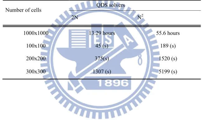
Table 3-1 Comparison of computational expenses for QDS schemes using 2N and N2 dimensional reconstruction. ... 70  

Table 3-2 QDS scheme time cost in Euler-4-shocks interaction case. ... 71  

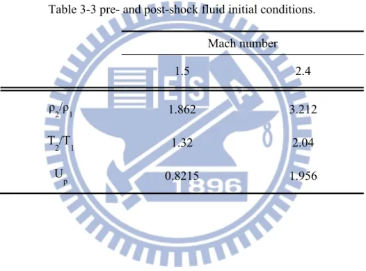
Table 3-3 pre- and post-shock fluid initial conditions. ... 72  

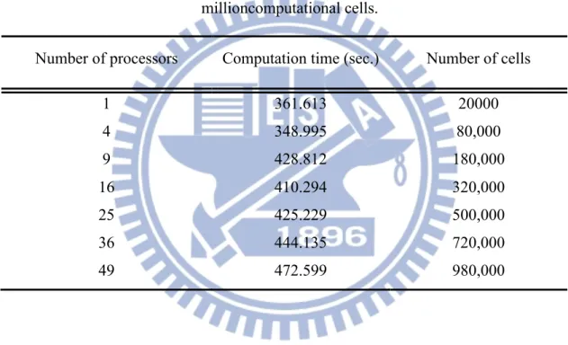
Table 3-4 Parallel Performance for a 2D shock-bubble problem with 2.4 million computational cells. ... 73  

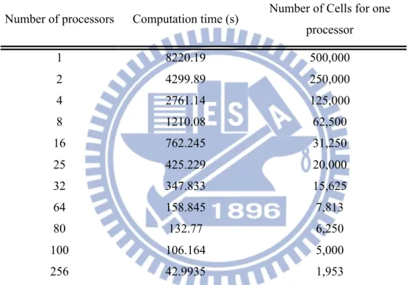
Table 3-5 Parallel computation times for shock-bubble problem with 500,000 cells at 2000 time steps in simulation time 0.2. ... 74  

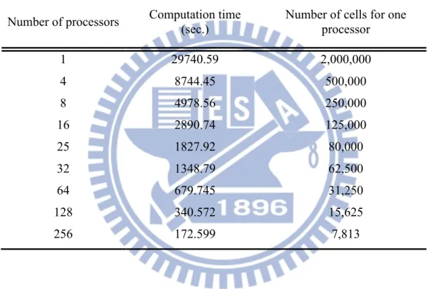
Table 3-6 Parallel computation times for shock-bubble problem with 2 million cells in 2000 time steps. ... 75  

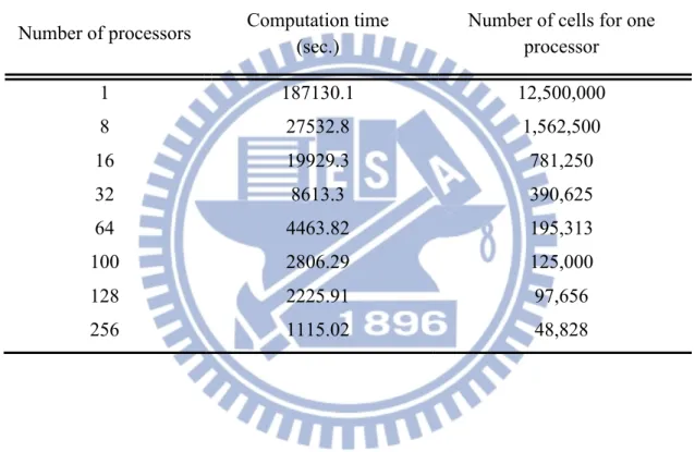
Table 3-7 Parallel computation times for shock-bubble problem with 12.5 million cells in 2000 time steps. ... 76  

List of Figures

Figure 2-1. Schematic showing the way fluxes of conserved quantities between source and destination cells are calculated using the “overlap” function in QDS [Smith et al., 2009]. ... 77  

Figure 2-2. Flowchart describing 2N-QDS particle computation with gradient inclusion. ... 78  

Figure 2-3. The special reconstruction convention for current amount of conserved quantity Q in one cell. ... 79  

Figure 2-4. QDS flux procedure within a general (arbitrary) spatial reconstruction of conserved quantity Q. ... 80  

Figure 2-5. Flowchart describing QDS particle computation with gradient inclusion. .. 81  

Figure 2-6. Two-dimensional motion of a single QDS particle showing “sub-particle” contributions. ... 82  

Figure 2-7. Three-dimensional motion of a single QDS particle showing “sub-particle” contributions. The green parallelogram is presented the concept in two-dimensional. ... 83  

Figure 3-2. The shock tube problem as computed by pre-QDS method with a uniform grid of 200 zones. The results were discussed thedifference to the QDS 1st ~3rd method and Riemann solver using MINMOD limiter at time 0.1. ... 85  

Figure 3-3. The interaction of two blast wave computed by the QDS method with 400 grids at t = 0.0038. The solid black line is WENO (fifth order) scheme with 10,000 grids. ... 86  

Figure 3-4. Density profile of the shock-acoustic-wave case at t = 1.8. The solid black line is WENO-3 (fifth order) with 2000 grids compared with QDS method which without limiter form 1st order to 3rd order. ... 87  

Figure 3-5. The structure of shock bubble interaction. ... 88  

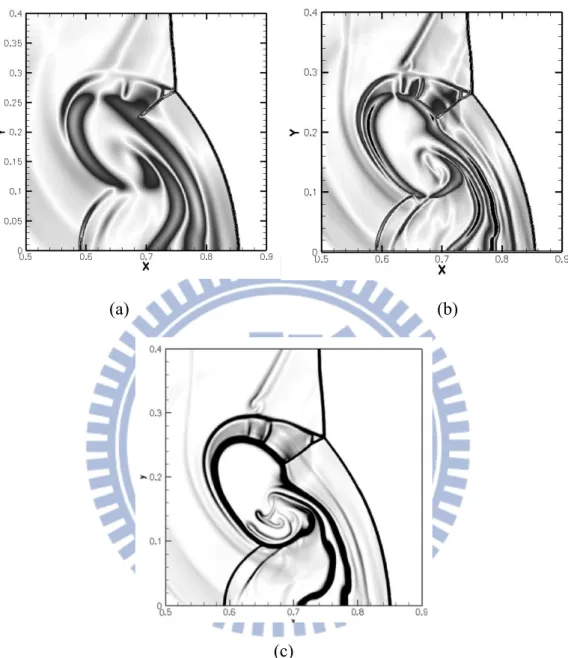
Figure 3-6. Zoom of shock-bubble Schlieren image with 1000×500 cells at time of 0.2. QDS 2nd order (a) 2N method with van Leer’s limiter, (b) N2 method, and (c) 2nd order TVD result presented in [Čada et al., 2009] using the same

resolution. ... 89  

Figure 3-7. Zoom of Schlieren image of shock bubble problem at time of 0.2; (a) QDS-N2 method with 300×100 cells; (b) QDS-2N method with 300x100 cells; (c) QDS-2N method with 450×150 cells; (d) QDS-2N scheme with 600×200 cells. ... 90  

Figure 3-8. The initial conditions for the first problem of Euler-4 shocks interaction. .. 91  

Figure 3-9. Zoom of density contour line of Euler-four-shocks problem. Comparing the second-order QDS-N2 method (a) using 100×100 grids with MC limiter and 2N method using 100×100 grids (b) and 200×200 grids (c), 300×300 grids (d) with MC limiter at time of 0.4. ... 92  

Figure 3-10. Zoom of the density contour lines of Euler four shocks problem. (a) the 2nd order TVD-MUSCL method taken from Čada [Čada et al., 2009] using 1000x1000 points, CFL=0.8. (b) The third-order QDS-N2 method used 1000x1000 grids with MC limiter at time of 0.8. (c) The third-order QDS-2N method used 1000x1000 grids with MC limiter. ... 93  

Figure 3-11. The initial conditions for the second problem of Euler-four-shock

Figure 3-12. Density profile of the four contacts problem for second-order

TVD-MUSCL method taken from [Čada et al., 2009]. ... 95  

Figure 3-13. Density contour obtained from QDS N2 solver (a) and 2N solver (b) by using 1000×1000 cells, 2nd _{order method with MINMOD limiter. The CFL}

number is 0.5. Level form 0 to 2.4 at 0.05 interval of line. ... 96  

Figure 3-14. Density contour obtained from QDS-2N solver with 5 particles (a) and 9 particles in each direction (b);QDS-N2 method with 5 particles (c) and 9 particles in each direction (d) by using 1,000×1,000 cells, 2nd _{order method}

with MINMOD limiter at time of 0.8. The CFL number is 0.5. Level form 0 to 2.1 at 0.05 interval of line. ... 97  

Figure 3-15. Density contour obtained from QDS-N2solverusing (a) 2,000×2,000and (b) 3,000×3,000 cells, 2nd _{order method with MINMOD limiter at time of 0.8.}

The CFL number is 0.5. Level form 0 to 2.1 at 0.05 interval of line. ... 98  

Figure 3-16. Geometry and boundary conditions for the Mach 3 flow over a forward facing step in a wind tunnel. All boundaries with exceptions to the inflow and outflow are secularly reflective. The outflow boundary is calculated through interpolation of states of interior cells. ... 99  

Figure 3-17. Contour of density at 4.0s for Mach 3 flow over a foeward facing step in a wind tunnel. Compare the 2nd order QDS-2N method (top) and QDS-N2 method (middle) for 600×200 grids. (buttom) The result of Keats and Lien [Keats et al., 2004] ... 100  

Figure 3-18. Structure of the perturbed region behind a diffracting shock wave, defined by from Skews [1967]. ... 101  

Figure 3-19. The output for compulsory figure for shock wave diffraction (by Takayama [1991]). ... 102  

Figure 3-20. The initial geometry of the shock wave diffraction over degree sharp corner. ... 103  

Figure 3-21. Schematic of moving shock waves [Anderson, 1990]. ... 104  

Figure 3-22. The density contours of the shock wave diffracting over 90 degree sharp corner with 400 × 400 grid, Ms=1.5. (a) the second-order TVD extension of

Godunov method [Takayama et al., 1991]. (b) the second-order QDS-2N method and (c) the second-order QDS-N2 method with MC linter, CFL=0.5. ... 105  

Figure 3-23. Schlieren image of the shock wave diffracting over a 90 degree sharp corner, Ms=1.5. (a) the experimental result made form Ritzerfeld et al.

[Takayama et al., 1991]. (b) second-order QDS-2N method and (c) QDS-N2 method with 400 × 400 cells, MC limiter, CFL=0.5. ... 106  

Figure 3-24. Vorticity magnitude contours compared (a) exact solution and two result using 2nd order (b) QDS 2N method and (c) QDS N2 in 800×800 uniform cells. All results are taken the CFL number to 0.1. ... 107  

Figure 3-25. The vorticity profiles along the central line passing through the vortex. The comparison contained the exact solution (blue squeal-symbol line), the QDS-N2 method using160×160 cells (red line), 800×800 cells (black dash-dot line), and 2N method using 800×800 cells (purple long-dash

line),1600×1600 cells (green doted line). Two method s are computed in MC limiter and CFL=0.1 at time 8.0. ... 108  

Figure 3-26. The three-dimensional geometry of the Mach 2 flow over a pillar. ... 109  

Figure 3-27. The Density contour of the Mach 2 flow over a pillar obtained using the second-order QDS-N2 method (a) in two-dimension with 200 × 200 cells; (b)

in three-dimension with 200 × 200 × 100 cells. The CFL factor is 0.5 using MINMOD limiter. ... 110  

Figure 3-28. The three-dimensional geometry of the Mach 2 flow over a square block. ... 111  

Figure 3-29. The Density contour of the Mach 2 flow over a square block obtained using the second-order QDS-N2 method with 200 × 200 × 100 cells (a) in x-y surface; (b) in x-z surface. The CFL factor is 0.5 using MINMOD limiter. ... 112  

Figure 3-30. Parallel Performance of a 2D shock-bubble interaction with 2.4 million computational Cells. ... 113  

Figure 3-31. Strong scaling performance in the QDS-N2 method with 500,000 cells on various massively parallel systems. ... 114  

Figure 3-32. Strong scaling performance in the QDS-N2 method with 2 million cells on various massively parallel systems. ... 115  

Figure 3-33. Strong scaling performance in the QDS-N2 method with 12.5 million cells on various massively parallel systems. ... 116  

Figure 4-1 The value of mass flux for the difference of 2N and N2 method. (a) The case 1 with the gradient 1.0e-5; (b) case 2 with the gradient 1.0e-6. ... 117  

Figure 4-2. The value of momentum flux in x-direction for the difference of 2N and N2

method. (a) The case 1 with the gradient 1.0e-5; (b) case 2 with the gradient 1.0e-6. ... 118  

Figure 4-3. The value of momentum flux in y-direction for the difference of 2N and N2 method. (a) The case 1 with the gradient 1.0e-5; (b) case 2 with the gradient 1.0e-6_{. ... 119}  

Figure 4-4. The value of energy flux for the difference of 2N and N2 method. (a) The case 1 with the gradient 1.0e-5; (b) case 2 with the gradient 1.0e-6. ... 120  

Figure 4-5. The value of energy flux for the difference of 2N and N2 method at the low density range. (a) The case 1 with the gradient 1.0e-5_{; (b) case 2 with the}

gradient 1.0e-6. ... 121  

Figure 4-6. Contour profile of Shock-bubble interaction. QDS-N2 2nd order method using 1700×500 cells with MC limiter at time of 0.2. (a) Density, (b)

temperature, (c) velocity in x-direction and (d) velocity in y-direction. .... 122  

Figure 4-7Shock-bubble Schlieren image with 1700×500 cells at time of 0.2. QDS 2nd

order (a) 2N scheme with van Leer’s limiter, (b) N2 scheme. ... 123  

Figure 4-8. The density contour obtianed using (a) the 2N method; (b) the N2 _method

with MC limiter, CFL=0.5, 1700×500 cells. ... 124  

Figure 4-9. The temperature contour obtianed using (a) the 2N method; (b) the N2

method with MC limiter, CFL=0.5, 1700×500 cells. ... 125  

Figure 4-10. contour profile of N2 method. (a)Density, (b) temperature, (c) velocity in x-direction and (d) velocity in y-direction. ... 126  

Figure 4-11. Contour of density at 4.0s for Mach 3 flow over a foeward facing step in a wind tunnel. Compare the 2nd order QDS-2N method (top) and QDS-N2 method (middle) for 600×200 grids. (buttom) The result of Keats and Lien [Keats et al., 2004] ... 127  

Figure 4-12. Contour of temperature obtained using second-order QDS-2N (top) and QDS-N2 method using 4 simulation particles for Mach 3 flow over a forward facing step in a wind tunnel. ... 128  

Figure 4-13. Schlieren image of the shock wave diffracting over a 90 degree sharp corner, Ms=2.4. (a) The experimental result made form Ritzerfeld et al.

[Dyke, 1997]. (b) the second-order QDS-2N method, and (c) QDS-N2 method with 1000 × 1000 cells, MC limiter, CFL=0.2. ... 129  

Figure 4-14. Density contours of Mach 2.4 shock diffraction using the second-order 2N method (top) and the N2 _{method with 1000×1000 uniform grids. The CFL}

number uses 0.2 with MC limiter. ... 130  

Figure 4-15. Temperature contours of Mach 2.4 shock diffraction using the second-order 2N method (top) and the N2 method with 1000×1000 uniform grids. The CFL number uses 0.2 with MC limiter. ... 131  

Figure 4-16. Velocity contours of Mach 2.4 shock diffraction using the second-order 2N method (top) and the N2 method with 1000×1000 uniform grids in

x-direction. The CFL number uses 0.2 with MC limiter. ... 132  

   

Nomenclature

N the number of terms

V the cell volume ρ the density,

u the bulk (or mean) flow velocity

v the velocity in y-direction T temperature

p pressure

E the total energy

e internal energy

p(x) the probability density ͘p momentum component

w weights of the Gaussian quadrature

q abscissas of the Gaussian quadrature

H the roots of the Hermite polynomials

FMASS total flux of mass from particle in a one-dimensional

FMOM total flux of momentum from particle in a one-dimensional

FENG total flux of energy from particle in a one-dimensional

∆t the simulation time step ∆x the cell size in x direction ∆y the cell size in y direction

mJ the particle mass

vJ the particle velocity

theparticle internal energy

J

σ = (RT)1/2 in a given source cell.

ξ The total number of degrees of freedom Ω the number of simulated degrees of freedom

ΔxL the location in the cell from where the flow properties are taken

Nx the total flux in x-direction for QDS-2N method

Ny the total flux in y-direction for QDS-2N method

A the overlap area

mflux mass fluxes contributed to the destination cell and subtracted from the source

cell

Eflux energy fluxes contributed to the destination cell and subtracted from the source

cell

px,flux momentum fluxes contributed to the destination cell and subtracted from the

source cell in x-direction

py,flux momentum fluxes contributed to the destination cell and subtracted from the

source cell in y-direction

AS the source cell area

qj(max) the maximum value of the particle abscissas

Q the value of a conserved property

X the boundary in the x-direction

Y the boundary in the y-direction Z the boundary in the y-direction

the average value of Q the equivalent flux limiter

F the phase space velocity distribution function

1 ) 1 ( 2 ₋ − = γ ξ Q φ

M The net of mass fluxes for analytical equation

m′ the value of mass with 2nd order method

P′ the value of momentum with 2nd order method

E′ the value of energy with 2nd ordermethod

m the total mass, momentum and energy at the source cell

P the total momentum at the source cell ∆ the difference of the value

β the constant value

2

m kT

β =

r position

mo the mass of the molecular

no the number of molecular per unit configuration-space volume

Superscripts

J the index for particle

Subscripts

k the index for particle in the y-direction

J the index for particle in the x-direction

i the cell position

x the element in x-direction

y the element in y-direction

z the element in z-direction

L left hand side

T top side

I inlet

O outlet

c the value of Q at the cell centre the value of Q

s the existing average value of the source cell

tr The flux out value of average conserved quantity successfully moving from the source cell into the destination cell (denoted by )

1 the mass flux 2 the momentum flux 3 the energy flux

N2 the value taken from QDS- N2 method

2N the value taken from QDS-2N method

F the gradient calculated using forward differences.

Chapter 1

Introduction

1.1 Background and Motivation

There are a number of approaches for the simulation of gas flows, depending on the nature and level of rarefaction of the flow. Computational fluid dynamics (CFD) typically uses the finite volume method to solve a set of discretized governing equations, usually the Euler or Navier-Stokes equations. Contemporary finite-volume CFD divides the computational domain into a grid of cells, and fluxes of mass, momentum, and energy are calculated through the interfaces between these cells. This technique suffers from the major disadvantage that the poor alignment of the grid with the flow field may result in large errors for some important flows (e.g., explosive blast wave), since fluxes can only occur between elements that share an interface, i.e., no reflection of the true-direction nature of the gas flow. Thus, CFD requires a careful grid design to ensure accurate results, convergence, and stability.

1.1.1 Direct Simulation Monte Carlo Method

The direct simulation Monte Carlo (DSMC) method has become the gold standard for stochastic flow field simulation. Arguably, this method has been the most successful for simulating rarefied gas flows since its development by Bird in the 1960s [Bird, 1994]. In the DSMC method the ballistic motion of the particles and their collisions are decoupled by moving the particles over a time step that is smaller than their mean collision time, indexing the particles to within a grid having dimensions that are smaller than the mean free path and then choosing collision partners from within this grid.

The DSMC algorithm requires the use of random numbers and is thus subject to statistical scatter and requires averaging over a large number of time steps to reduce the scatter in the sampled macroscopic properties. However the fluxes of properties in DSMC are “true-direction” since a particle can carry its mass, momentum, and energy between any two points in the flow field, not just between elements that share an interface. Furthermore, DSMC handles non-equilibrium effects by stochastically performing collisions between selected collision pairs, thus allowing gradual and selective transfer of momentum and energy.

In the high collision rate limit of DSMC, the particle velocity distributions approach that of the Maxwell-Boltzmann equilibrium distribution and moments of the Boltzmann equation reduce to the Euler equations [Gombosi, 1994].

1.1.2 Quiet Direction Simulation Monte Carlo Method

Albright et al. [2002] developed the quiet direction simulation Monte Carlo (QDSMC), a method for modeling plasmas. They subsequently applied this method to the simulation of Eulerian fluids for Sod’s one-dimensional shock tube problem and a simple two-dimensional blast wave problem. Since then little further work has been done, the only example being by Peter [Gombosi, 1994] who applied a random time step to the movement of simulation particles for simulating a typical diffusion equation. Unlike the DSMC method, there is no random number (or Monte Carlo) component to the algorithm. In the QDSMC method, the effect of sampling using random numbers is replaced by using the weights and abscissas of a Gauss–Hermite quadrature. Thus, it is valid only when thermal equilibrium can be assumed. Moreover, this method is a particle-based Euler solver that exhibits negligible statistical scatter and has a large dynamic range.

1.2 Literature Survey

Bird [Bird, 1994] showed that the DSMC method essentially provides a statistical solution to the Boltzmann equation, and Wagner [Wagner, 1992] proved mathematically that DSMC provides a solution to the Boltzmann equation as the number of simulated particles approaches the number in the actual system. This method was used to model the relaxation of a non-equilibrium gas towards the equilibrium distribution [Bird, 1963] and since that time it has been used in a wide array of applications including CVD reactor modeling [Coronell et al, 1992], hypersonic flight simulations [LeBeau et al., 2001], supersonic jet studies [Boyd et al., 1994; Teshima et

al., 2001], microfluidic simulations [Karniadakis, 2002], and modeling of molecular

pumps [Kwon et al., 2006]. The method has grown increasingly sophisticated and powerful as improved algorithms, intermolecular collision models, gas-phase chemistry and boundary conditions have been developed and implemented.

Since the development of DSMC by Bird to solve the Boltzmann equation statistically, a large number of continuum kinetic theory based-schemes have emerged that follow a similar path.In 1980, Pullin proposed the equilibrium flux method (EFM) as an analytical equivalent to the equilibrium particle simulation method (EPSM), which is a direct simulation method where particles are forced to assume the Maxwell-Boltzmann equilibrium velocity probability distribution function instead of performing collisions [Pullin, 1980]. Later, Smith et al. [Smith et al., 2008] proposed a general form of the EFM method known as the true direction equilibrium flux method (TDEFM), which more accurately captures the transport mechanism employed by EPSM. Fluxes calculated by TDEFM represent the true analytical solution to the molecular free flight problem, under the assumption of thermal equilibrium and uniformly distributed quantities. The calculated fluxes are valid for any size time step,

and the algorithm is unconditionally stable, although the kinetic Courant-Friedrich-Levy (CFL) number should be kept below unity to ensure physical correctness. The primary disadvantage to TDEFM is the large computational cost associated with the evaluation of the numerous exponential and error function evaluations.

As mentioned previously, Albright et al. [2002] developed the QDSMC method, a numerical scheme for the solution of the Euler equations. They subsequently applied QDSMC to the simulation of Eulerian fluids for problems like shock tube flow and blast wave propagation. In this method, the integrals encountered in the TDEFM formulation are replaced by approximations using Gaussian numerical integration, effectively replacing the continuous velocity distribution function with a series of discrete velocities. The method was later renamed the quiet direct simulation (QDS) method due to the lack of stochastic processes and was extended to second order spatial accuracy. The lack of complex mathematical functions results in a computationally very efficient scheme with considerably higher performance than EFM while maintaining the advantages of true directional fluxes like TDEFM.

Due to the assumption of unrestricted motion during free flight, each of the above-mentioned kinetic solvers has a large amount of (cell-size-based) numerical diffusion. To combat this dissipation, a common strategy, employed in more conventional finite volume methods, is to apply higher-order reconstruction of properties or fluxes. Macrossan [Macrossan, 1989] applied EFM using higher order spatial extensions, while Smith [Smith, 2008] attempted the analytical inclusion of gradients into true-direction volume-to-volume fluxes, only to find that the complete analytical inclusion of gradient terms in the TDEFM flux expressions is impossible. Smith et al. [Smith et al., 2009] reduced the numerical diffusion by applying “simplified” flux reconstruction at the

interface. This method, known as QDS-2N, improves the original QDS to be almost second order in spatial accuracy.

The particle-based QDS-2N method is easily extended to multi-dimensions and multi-species. It is computationally inexpensive, easily implemented on parallel computers and, since it is a particle-based method, and does not require direction decoupling. The major disadvantage is that the scheme is inherently very diffusive. The particle-based Euler solver has two advantages. First, hybridization between the solver and a pure DSMC solver which is capable of simulating the non-continuum regions of flow is relatively simple. Several authors, including Macrossan [Macrossan, 2001], Chen [Chen, 2003], Smith [Smith, 2003] and Wu [2003], have developed such particle-based hybrid methods. The second major advantage is that particle-particle-based methods can exchange fluxes between any two cells on the grid for any given time step. Direction decoupled CFD methods only allow fluxes to be exchanged between cells sharing a common interface. This physically unrealistic situation results in non-physical results in CFD simulations [Smith et al., 2008: Cook, 1998].

The second-order QDS-2N method was applied by Cave [Lim et al., 2010: Cave, et

al., 2010] to simulate highly unsteady low pressure flows encountered in a pulsed

1.3 Specific Objectives of this Thesis

Based on the preceding discussion of studies related to the QDS-2N method, it is clear that further numerical study is needed to improve the accuracy of the QDS-2N method and, consequently, lead to more effective applications.

In this thesis, we extend the second-order QDS algorithm (QDS-2N) [Smith et al., 2009] to flux reconstruction through true-direction polynomial multi-dimensional reconstruction of conserved properties across each cell width; this method is called QDS-N2_.

The specific objectives and organization of this thesis can be summarized as follows:

1. To improve the QDS-2N method by first studying its advantages and disadvantages. Flux reconstruction calculated using QDS-2N neglects neighbourhood cells when calculating diagonally cells. (Chapter 2)

2. To develop a QDS-N2method for solving Euler’s equation for inviscid fluid flow. The fluxes of conserved properties are calculated by a sum of weighted moments over the polynomial spatial reconstruction of mass, momentum, and energy across the cell width. The particle properties are updated, considering the average value of the conserved quantity between the region bounds, which are required in translational directions and the application of splitting. (Chapter 2) 3. To develop the QDS-N2 method in three-dimensions. (Chapter 2)

4. To apply the QDS-N2 method to a numerical problem and an experimental case. Various numerical methods, including Riemann solvers and total variation diminishing (TVD) methods, were compared as a benchmark. (Chapter 3)

6. To develop the parallel QDS-N2method for large-scale applications such that the computational time problem is reduced efficiently. The scheme includes weak scaling and strong scaling. (Chapter 3)

7. To analyzedifferences associated with the 2Nmethod and compare QDS-2Nto QDS-N2_{.This involves measurements to reveal differences between the}

two methods and provides information to determine which problem will be considered first. (Chapter 4)

8. The concluded by summarizing the major findings found in this thesis and outlining the recommendations for the future work. (Chapter 5)

Chapter 2

Numerical Methods

2.1 Overview of Euler Equation Solver

The Euler equations describe how the density, velocity, and pressure of a moving fluid are related. The Euler equations directly represent conservation of mass, momentum, and energy, and correspond to the Navier-Stokes equations without viscosity and heat conduction terms. Eq. (1) shows a two-dimensional formulation of the Euler equations.

Continuity:

( ) ( )

u v 0 t x y ρ ρ ρ ∂ ∂ ∂ + + = ∂ ∂ ∂ X-momentum:

( )

( )

2 u uv u P t x y x ρ ρ ρ ∂ ∂ ∂ _{+ + = −}∂ ∂ ∂ ∂ ∂ (1) Y-momentum:

( )

( )

2 v uv v P t x y y ρ ρ ρ ∂ ∂ ∂ _{+ + = −}∂ ∂ ∂ ∂ ∂

Although the continuity and momentum equations have been derived in the past, the energy equation has been included in the Euler equations in fluid dynamics literature [Anderson, 1995].

2.1.1 Computational Fluid Dynamics

Engineers made further approximations and simplifications to the equation set until they had a group of equations that they could solve. Recently, high speed computers have been used to solve approximations to the equations using a variety of techniques,

such as finite difference, finite volume, finite element, and spectral methods. This area of study is called CFD.

The Euler equation for the conservation of continuity, momentum and energy equation is:

(

)

(

)

2 2 0 u v u P uv u uv v P v t x y u E p v E p E ρ ρ ρ ρ ρ ρ ρ ρ ρ ρ ρ ρ ρ ρ ⎛ ⎞ ⎛ ⎞ ⎛ ⎞ ⎜ ⎟ ⎜ ⎟ ⎜ ⎟ ₊ ∂ _{⎜ ⎟ +} ∂ _{⎜ ⎟+} ∂ _{⎜ ⎟=} ⎜ ⎟ ⎜ ⎟ ⎜ ⎟ + ∂ ∂ ∂ ⎜ ⎟ ⎜ ⎟ ⎜ ⎟ _{⎜ + ⎟ ⎜ + ⎟} ⎝ ⎠ ⎝ ⎠ ⎝ ⎠ (2) where 1

(

2 2

)

2

E e= + u +v is the total energy and e is internal energy e=e(T).For a perfect gas, internal energy is only dependent on temperature. Pressure is presented by p

= (γ - 1)ρe with γ = cp/cυ the ratio of specific heats (γ = 7/5 for air).

Most numerical schemes for solving Euler equations are built around the Riemann solver. For example, Godunov technique provided two and three dimension applications in new finite volume numerical schemes and total variation diminishing (TVD) properties [Toro, 2009; LeVeque, 2004], and achieved second-order accuracy. Although, such numerical methods were generally accurate, they incurred high computational costs. However, approximate numerical schemes that reduce computational costs are not only less accurate and less robust but are also based on solutions of a Riemann problem. More extensive introductions to numerical method for the Euler equations ware given by Godlewski and Raviart [1996], Kroner [1997], Laney [1998], Majda [1984], Toro [1997], Smoller [1983], and Hirsch [1990].

2.1.2 Kinetic Method

The classical kinetic theory of gas emerged from a combination of mechanics and statistics. The motions of molecules are described by probability rather than their

pressure, temperature, and a generalized equation of state for gases, and 2) transport properties (velocity, thermal conductivity, diffusion coefficients) based on first principles.

The kinetic method can be introduced by the Boltzmann equation, which is used in the study of a collection of particles in non-equilibrium statistical mechanics. The Boltzmann equation was devised by Ludwig Boltzmann in 1872 [Lerner et al., 1991]. The equation is a phase space of system that contains seven variables: three coordinates for position coordinates x, y, z, where each coordinate is parameterized by time t and three for each momentum component ͘px, ͘py, ͘pz and each coordinate is parameterized by

time t. The volume element for position r and momenta ͘p can be expressed as follows:

d3rd3͘p = dx dy dz d͘px d͘py d͘pz (3)

For one chemical species, the Boltzmann equation can be written as follows:

i i coll i i F F F F v a t x v t

δ

δ

∂ ₊ ∂ ₊ ∂ _{= ⎜ ⎟}⎛ ⎞ ∂ ∂ ∂ _{⎝ ⎠} (4)

where F is the phase space velocity distribution function which is the density of particles in the d3_rd3͘_{p phase space volume element around the phase space point (r, ͘p).}

∂F/∂t is the total time derivative of the phase space distribution function, and₍δF/δt_)coll

= rate of change of the phase-space distribution function due to collisions.

The Euler equation can be described using by kinetic theory. Here the conservation equation of mass, momentum and energy are derived as follows:

(

)

₍

₎

(

)

(

)

(

)

0 0 0 3 3 5 0 2 2 2 o o o o o o o o o o m n m n t u m n m n u u p m n a t p u p p u t ∂ + ∇ ⋅ = ∂ ∂ + ⋅∇ + ∇ − = ∂ ∂ + ⋅∇ + ∇ ⋅ = ∂ (5)

where mo is the mass of the molecular object and no is the number of molecule per unit

configuration-space volume. Because the Euler equations are non-linear hyperbolic equations, the shock waves are generally described by these equations. Several highly successful algorithms have been developed to solve such problems [Jameson, 1986; MacCormack et al., 1975; Jameson et al., 1981].

In addition to the Boltzmann equation, Maxwell-Boltzmann distribution also contributed to the kinetic theory of gasses. This distribution was first carried out in 1859 and was named after James Clerk Maxwell and Ludwig Boltzmann. The distribution function can be expressed as follows:

(

)

32

(

2 2 2

)

, ,

vx vy vz x y z

f v v v

β

e

β

π

− + +

⎛ ⎞

= ⎜ ⎟

_{⎝ ⎠}

(6) where the constant value

2

m kT

β =

This distribution function assumes the ideal gas is isotropic and that velocity is statistically independent. This means that there is no preferred direction and the function is independent of the orientation of the coordinate system. The gas for this distribution is close to thermodynamic equilibrium. An understanding of the Maxwell-Boltzmann distribution function is essential when studying the QDS method. The detail will be discussed in the next section (subchapter 2.2).

2.2 Quiet Direct Simulation (QDS) Method

[Albright et al., 2002]

The normal random variable N(0,1) is defined by the probability density:

(7) by using a Gaussian quadrature approximation, the integral of Eq.(7) over its limits can be approximated by:

p x

( )

=e

−x2

2 2π

( )

( )

2 2 1 2 x N J J J e f x dx w f q π − ∞ = −∞ ≈

∑

∫

(8)

where wJ and qJ are the weights and abscissas of the Gaussian quadrature (also known

as the Gauss-Hermite parameters) shown in Table 1, and N is the number of terms. The abscissas are the roots of the Hermite polynomials, which can be defined by the recurrence equation:

(9) where H-1=0, and H0=1. The weights can be determined from:

( )

1 2 2 1 2n ! J n J n w n H q π − − = ⎡ ⎤ ⎣ ⎦ (10)

The moment of the form are represented as

( )

2 2 1 2 N r r J J J e d w q υ υ υ π − ∞ = −∞ ≈

∑

∫

(11) where r=0,1,…, 2N-1.

The particle simulation of fluid behaviour involved random variables which governed by stochastic differential equations of motion. For example, the one-dimensional Ornstein-Uhlenbeck (OU) equations describe the random dynamics of a particle of mass relaxing at a rate γ to the local fluid velocity u and temperature

2 kT =mσ_υ shown as: x dx=υ dt (12)

(

)

₂ 2 _(0,1) x x dυ = −γ υ −u dt+ γσ_υdt N (13) where N(0,1) is random variable. When eq.(13) in the initial condition υ_x

( )

0 =υ_x0 ,it can be solved [Gardiner, 1985] from following equation:

( )

(

0

)

1

( )

0,1

t t

x t u e γ x u υ e γ N

υ _{Δ = +} − Δ υ _{− +}σ ₋ − Δ ₍₁₄₎

In the thermalization γ∆t >>1, eq. (13) can be described as u+σ_υN

( )

0,1 drawn H_n+1(q)= 2qH_n − 2nH_n−1

As same as DSMC calculations to split particle transport and particle thermalization into two distinct operations, we presented operations by differential OU process which denoted with subscript tr and th respectively as follows:

(

)

2 0 0 2 (0,1) x x tr x _th dx dt d _{u dt υdt N} υ υ _{γ υ γσ} ⎛ ⎞ ⎛ ⎞ ⎛₌ ⎞ _{= ⎜ ⎟} ⎜ ⎟ ⎜ ⎟ _{⎜− − + ⎟} ⎝ ⎠ ⎝ ⎠ _{⎝ ⎠} (15)

The transport differential operator describes particle free streaming, while thermalization operator drives particle velocities toward u+σ_υN

( )

0,1 without changing their positions. In the QDS algorithm, the part of tr preforms particle properties i.e. masses, momenta, special internal energies in each mash; The part of th represents each particle which is advanced to a new position. Those parts are established local thermodynamic equilibrium throughout the fluid.

The net fluxes of mass, momentum and energy of a cell are given by the sum of individual flux contributions from all the particles flowing in and out as follows:

1 1

M N

J J

MASS MASS MASS

J _in J _out F F F = = ⎛ ⎞ ⎛ ⎞ =_{⎜ ⎟} −_{⎜ ⎟} ⎝

∑

⎠ ⎝

∑

⎠ , 1 1 M N J J

MOM MOM MOM

J _in J _out F F F = = ⎛ ⎞ ⎛ ⎞ =_{⎜ ⎟} −_{⎜ ⎟} ⎝

∑

⎠ ⎝

∑

⎠ , 1 1 M N J J

ENG ENG ENG

J in J out F F F = = ⎛ ⎞ ⎛ ⎞ =_{⎜ ⎟} −_{⎜ ⎟} ⎝

∑

⎠ ⎝

∑

⎠ (16)

where , and is the individual mass flux, individual momentum and individual energy from particle J respectively, M and N is the number of inflow and outflow particles respectively into the cell under consideration. Each of the individual contribution (with first order spatial accuracy) can be described by the expressions, e.g., in one-dimensional case:

(17)

where the particle mass mJ, particle velocity vJ, and particle internal energy are

expressed as: (18) J MASS F J MOM F J ENG F FJ MASS= v_JΔt Δx mJ FMOM J ₌ vJΔt Δx mJvJ FENG J ₌ vJΔt Δx mJ 1 2vJ 2 _+ε J ⎡ ⎣⎢ ⎤ ⎦⎥ J

ε

π ρ J J xw m = Δ v_J = u + 2σq_J

(

)

2 2 σ ξ εJ = − Ω

where ρ is the density, u is the bulk (or mean) flow velocity, and σ = (RT)1/2 in a given source cell. Note R is the universal gas constant, and T is the gas temperature. The total number of degrees of freedom ξ is defined as and Ω is the number of simulated degrees of freedom (e.g., Ω = 1 for one dimensional flow). In the existing QDS-2N [Smith et al., 2009], the values of ρ, u, and σ employed in QDS particle initialization are taken from reconstructions based on linear variations. Despite fluxes being true direction in nature, the reconstructions performed by previous implementations are direction decoupled – i.e. a flux is computed through the product of (separate) fluxes previously computed (for 2D flow) in the x and y directions. For the 2D case, the particle mass and velocities in Eq. (9) become:

J K JK x yw w m ρ π Δ Δ = ₂ 2 J x J v = +u

σ

q ₂ 2 K y K v = +u

σ

q (19)

where there are K=1,…, M particles in the y-direction and the definition of other variables are the same as those in 1D case. The internal energy remains identical to the 1-D case, allowing for a corresponding increase in Ω to account for the extra simulated dimension. The fluxes from sources cell to any arbitrary destination cell can be calculated by the particle position distributions. The fluxes of mass, momentum and energy, which are based on the proportion of the overlapped area to the area of the original cell, are given by:

MASS JK s A F m A = MOM X JK J s A F m v A − = MOM Y JK K s A F m v A − =

(

2 2

)

1 2 ENG JK J K JK s A F m v v A

ε

⎡ ⎤ = _⎢ + + _⎥ ⎣ ⎦ (20)

where A is the overlapped area as u×v×dt2 _{and A}

s is the source cell area as dx×dy.

1 ) 1 ( 2 − − = γ ξ

2.3 QDS-2N Method

In the QDS-2N algorithm used in the present study, the concept of QDS “particles” whose properties are interpolated onto a grid (as used by Albright et al. [2002] in their original development of the technique) is replaced by the concept of fluxes of a large number of particles uniformly distributed across the cell, as described by Smith et al. [Smith et al., 2008]. In this finite volume approach, quantities such as mass, momentum and energy are exactly conserved by tracking fluxes from source volumes to destination volumes. If the particle position distributions (i.e. gradients of density in the flow) are known, the flux from the source region to any arbitrary destination volume can be calculated.

In the present implementation of QDS-2N, the flux scheme employed by Smith et

al. [2009] is used for the efficient calculation of two dimensional, true direction fluxes.

Here the Nx fluxes in each coordinate direction are computed separately requiring the

calculation of 2N fluxes for the two-dimensional case.

In the second order scheme the gradients of cell velocity in the x-coordinate direction (du/dx), can be used to update the flux velocity:

2 2 J L v J du v u x q dx σ = + Δ + (21)

where ΔxL represents the location in the cell from where the flow properties are taken.

Fluxes moving to the right are assumed to take their quantities from the reconstructed state ΔxL = 0.5(Δx – vxj∆t) to the right of the cell canter, where ∆x is the cell size and ∆t

is the simulation time step. This corresponds to the displacement of the centre of mass of the flux which moves into the destination cell. Left moving fluxes have properties constructed in a similar fashion for which ΔxL = 0.5(–Δx – vxj∆t). The flux then moves

The total mass and energy associated with the particles in the particular “bucket” for the second-order case in the x-direction can be determined from the cell’s density (ρ), energy (E) and their respective gradients by:

L J J d x xw dx m ρ ρ π ⎛ _{+ Δ} ⎞_Δ ⎜ ⎟ ⎝ ⎠ = (22)

where wj are weights of the Gauss-Hermite quadrature, and:

(

)

2 2 L J d x dx σ ξ σ ε ⎛ ⎞ − Ω _⎜ + Δ _⎟ ⎝ ⎠ = Ω (23)

where Ω=2 for two-dimensional simulations. Any unused translational and other non-translational degrees of freedom are thus treated as internal structural degrees of freedom.

The amount of mass which fluxes to the new cell can be determined by multiplying Eq. (22) by vJ∆t /∆x. The gradients used in Eq. (21) to (23) are determined using the

MINMOD (Minimum Modulus) and the MC (Monotonized Central Difference) scheme [Van Leer, 1977]. Using density in the x-direction as an example, the gradient using the MC slope limiter is:

(24)

where the MINMOD scheme is:

(25)

It should be noted that when non-uniform grids are employed (for example, when adaptive mesh refinement and coarsening is employed) the fluxes must be calculated together (for a total of Nx*Ny fluxes). In this case, for a purely two-dimensional

⎥ ⎦ ⎤ ⎢ ⎣ ⎡ ⎟ ⎠ ⎞ ⎜ ⎝ ⎛ Δ − Δ − Δ − = + − + − x x MINMOD x MINMOD dx d i 1 i1_{, 2} i1 i _,2 i i1 2 ρ ρ ρ ρ ρ ρ ρ

[ ]

( )

( )

( )

⎪ ⎩ ⎪ ⎨ ⎧ < > < > < = ) ( AND ) 0 (SIGN IF ) ( AND ) 0 (SIGN IF 0 SIGN IF 0 , MINMOD a b ab b b a ab a ab b a

simulations, the amount of flux from one cell to another can be calculated trivially by determining the overlap area A=vJvk∆t2 (where there are k = 1,…,N fluxes in the

y-direction and vk is calculated in the same manner as Eq. (21) divided by the source cell

area AS = ∆x∆y, as shown in Figure 2-1. The mass m and the energy ɛ are thus given

by: L L J k Jk d d x y x yw w dx dy m ρ ρ ρ π ⎡ _{+ Δ}⎛ _{+ Δ} ⎞⎤_{Δ Δ} ⎢ ⎜ ⎟⎥ ⎝ ⎠ ⎣ ⎦ = (26)

(

)

2 L L Jk d d x y dx dy σ σ ξ σ ε ⎡ ⎛ ⎞⎤ − Ω _⎢ + Δ_⎜ + Δ _⎟⎥ ⎝ ⎠ ⎣ ⎦ = (27)

where ΔyL is calculated in a similar manner to ΔxL. Thus the amount of mass mflux,

energy Eflux and momentum in each coordinate direction px,flux and py,flux which must be

added to the destination cell and subtracted from the source cell are given by:

flux S A m m A = (28)

(

2 2

)

1 2 flux J k Jk S A E m v v A ε ⎡ ⎤ = _⎢ + + _⎥ ⎣ ⎦ (29) , flux x J S A p mv A = (30) , flux y k S A p mv A = (31)

A variable time step scheme is used to maintain the maximum kinetic Courant– Friedrichs–Levy (CFL) number in the domain below a desired value (usually ≤1). It is important to note that this CFL restriction is to maintain physical realism and is not related to the numerical stability of the scheme. For a two-dimensional or axisymmetric simulation, the CFL number is given by:

(

)

(

)

(

)

2 2 (max) 2 2 J u v q RT t CFL x y + + Δ = Δ + Δ (32)

where qj(max) is the maximum value of the particle abscissas (i.e. the value which gives

the maximum particle thermal velocity).

In the current implementation boundary conditions are handled using ghost cells. These cells can be used to represent walls, stream boundaries, inflow boundaries and zero-gradient outflow boundaries. The interaction of a gas with a wall is identical to the interaction of that flow with an adjacent cell having the same flow properties but a reversed flow direction normal to the wall. The basic description of the simulation processes for QDS-2N method is available in Figure 2-2.

2.4 QDS-N

2

Method

2.4.1 Spatial Reconstruction and Flux Calculation

In the current study, referring to Figure 2-3, the general extension to higher order in QDS in one-dimensional case is performed using a spatial reconstruction of the form:

(33)

where Q(x) is the value of a conserved property (mass, momentum, or energy) at a distance x from the left hand side of the cell, and integer n indicates the order of the reconstruction. Note Qc is the value of Q(x) at the cell centre. This value is calculated

from Q(x) integrating over the cell width divided by the cell width equalling to the existing average value of the source cell Q_s, presented below:

Q x

( )

= Qc+ dQ dx ⎛ ⎝⎜ ⎞⎠⎟_x=0.5Δx

(

x− 0.5Δx

)

+ d2Q dx2 ⎛ ⎝⎜ ⎞ ⎠⎟_x=0.5Δx x− 0.5Δx

(

)

2 2 + ...+ dn−1 Q dxn−1 ⎛ ⎝⎜ ⎞ ⎠⎟_x=0.5Δx x− 0.5Δx

(

)

n−1 n−1

(

)

!

( )

(

)

2 2

(

)

3 1 1 1 0.5 0.5 ... 2 6 R L R L X s _X R L x X c x X Q Q x dx X X dQ d Q Q x x x x x dx dx = = = − ⎡ ⎛ ⎞ ⎛ ⎞ ⎤ =_⎢ + _{⎜ ⎟} − Δ + _{⎜ ⎟} − Δ + _⎥ ⎝ ⎠ ⎝ ⎠ ⎣ ⎦

∫

(34)

By using our revised reconstruction, the bounds of integration are XL=0 and XR=∆x.

Then, Eq. (34) leads to:

2 2 4 4 1 1 2 4 1 2 1 ... 24 1920 ! 2 n n n c s n x d Q x d Q x d Q Q Q dx dx n dx − − − ⎛ ⎞ ⎛ ⎞ ⎛ ⎞ Δ Δ Δ ⎛ ⎞ = + _{⎜ ⎟}+ _{⎜ ⎟}+ + _{⎜ ⎟ ⎜ ⎟} ⎝ ⎠ ⎝ ⎠ ⎝ ⎠ ⎝ ⎠ (35)

Alternatively, Qc can be expressed as follows:

2 2 4 4 1 1 2 4 1 2 1 ... 24 1920 ! 2 n n n c s n x d Q x d Q x d Q Q Q dx dx n dx − − − ⎛ ⎞ ⎛ ⎞ ⎛ ⎞ Δ Δ Δ ⎛ ⎞ = − _{⎜ ⎟}− _{⎜ ⎟}− − _{⎜ ⎟ ⎜ ⎟} ⎝ ⎠ ⎝ ⎠ ⎝ ⎠ ⎝ ⎠ (36)

where n is assumed to be an odd number. This shows that the correction is only required when the scheme is third order (n = 3) accurate or higher, otherwise Q_c =Q_s (e.g., n=2). Thus, the complete correct form of the higher order reconstruction of Q(x) using Q_s contains additional terms on every even derivative:

( )

(

)

(

)

(

)

(

)

2 2 2 4 4 2 2 4 2 3 3 3 0.5 0.5 24 1920 2! 0.5 1 0.5 3! ! s n n n x x x d Q x d Q dQ d Q Q x Q x x dx dx dx dx x x d Q d Q x x dx dx n ⎛ Δ ⎛ ⎞ Δ ⎛ ⎞⎞ ⎛ ⎞ ⎛ ⎞ − Δ =⎜ − ⎜ ⎟− ⎜ ⎟⎟+⎜_⎝ ⎟_⎠ − Δ +⎜ ⎟ ⎝ ⎠ ⎝ ⎠ ⎝ ⎠ ⎝ ⎠ − Δ ⎛ ⎞ ⎛ ⎞ + _{⎜ ⎟} − Δ +_{⎜ ⎟} ⎝ ⎠ ⎝ ⎠ (37)

Specifically, as n=2, the above is reduced to the following form because ofQ_c =Q_s, as shown below: 2 2 2 1 ( ) ( 0.5 ) ( 0.5 ) 2! s dQ d Q Q x Q x x x x dx dx = + − Δ + − Δ (38)

The above reduces to exactly the same form as in QDS-2N [Smith et al., 2009]. Next, referring to Figure 2-4, the outgoing flux value of average conserved quantity successfully moving from the source cell into the destination cell (denoted by Q ) is: _tr