國立交通大學
管 理 科 學 系 碩 士 班
碩士論文
科技預測模型之檢測:廣泛的羅吉斯模型、費雪模型、
以及甘伯茲模型之比較
The Test of Technological Forecasting Models:
Comparison between Extended Logistic Model,
Fisher-Pry Model, and Gompertz Model
研 究 生:陳俊朋
指導教授:張力元 博士
科技預測模型之檢測:廣泛的羅吉斯模型、費雪模型、以及甘伯茲模
型之比較
The Test of Technological Forecasting Models: Comparison between
Extended Logistic Model, Fisher-Pry Model, and Gompertz Model
研究生:陳俊朋 Student : Chun-Peng Chen
指導教授:張力元 博士 Advisor: Dr. Charles V. Trappey
國立交通大學
管理科學系碩士班
碩士論文
A Thesis
Submitted to Institute of Management Science
National Chiao Tung University
in Partial Fulfillment of the Requirements
for the Degree of Master of Business Administration
June 2005
Hsinchu, Taiwan, Republic of China
中華民國九十四年六月
科技預測模型之檢測:廣泛的羅吉斯模型、費雪模型、以及
甘伯茲模型之比較
學生:陳俊朋 指導教授:張力元
國立交通大學管理科學系碩士班
摘要
這篇論文的目的主要是在檢測一個擁有可變動上限以及彈性轉折點的新模 型與其他以廣泛應用的科技預測模型之比較。科技預測對於決策者來說是非常好 的補助工具,它除了可以用來找尋科技替代的趨勢以及可能的產品發展的上限之 外,也可以被用來檢測產品生命週期的可能趨勢。因此,好的預測可以對未來的 趨勢提供一個良好的訊息。費雪模型以及甘伯茲模型是兩種廣泛應用的模型,而 且現今也有許多改良的模型被應用在各種科技預測的領域。 因此,這篇論文利 用預測圖形以及數理指標來檢測這三種模型的適用性。 本篇論文利用了日本家電產品的滲透率來做模型的比較,此外還利用數位 相機的像數的演進來做為實際檢測磨行事用性的依據。結果發現費雪模型在資料 點多且可達到百分之百的滲透率或替代率時有較好的預測性,而甘伯茲模型則在 當可以適當地找出適合的上限時有較好的表現。至於廣泛的羅吉斯模型不管在預 測或者是模型的配適上都有不錯的表現。 關鍵字:科技預測、廣泛的羅吉斯模型、費雪模型、甘伯茲模型The Test of Technological Forecasting Models: Comparison between
Extended Logistic Model, Fisher-Pry Model, and Gompertz Model
Student: Chun-Peng Chen Advisor: Dr. Charles V. Trappey
National Chiao Tung University
Department of Management Science
Abstract
The purpose of this thesis is to find a new technological forecasting model based on time-varied capacity and it has a flexible point of inflection. Technological forecasting is a good auxiliary tool to help managers make a decision whether in technological substitution or technological growth. It can also be used to find out the time that will reach the maximum growth rate and to know the possible trend of product’s life cycle. Consequently, a good forecasting can offer useful information to know the possible circumstances in the future. Fisher-Pry and Gompertz model are the most commonly used in this field, and many adapted models also based on their structure. Therefore, this thesis compares these models according to curves and mathematical criteria.
The penetration of durable goods is used to test these three models. The result shows that Fisher-Pry model can fit the data well in some long data sets which reached 100% of capacity and Gompertz model fits data well when the right capacity has been set and data set is asymmetric. The extended logistic model shows a better fit and forecast in most data sets.
Keywords: Technological Forecasting, Fisher-Pry model, Gompertz model, The
ACKNOWDGEMENT
This master thesis was written under the supervision of Management of Science
department at National Chiao Tung University. I am glad to finish this thesis eventually, and I want to thanks my good friends in Hsinchu including my girlfriend, Jenny. You brought me a lot of happiness in these two years. Although this thesis took me a lot of time and effort to finish it, I gained more in this process. Since Dr Trappey provided lots of information and advice during the research I would like to thank him for his support. Furthermore, I would like to thank my parents who encourage me to get the master degree.
Chun-Peng Chen National Chiao Tung University Hsinchu, Taiwan June 2005
TABLE OF CONTENTS
摘要...i
Abstract...ii
ACKNOWDGEMENT ... iii
TABLE OF CONTENTS...iv
LIST OF TABLES ...vi
LIST OF FIGURES ...vii
CHAPTER 1 INTRODUCTION ...1 1.1 Background...1 1.2 Problem Discussion ...2 1.3 Research Motivation ...4 1.4 Research Purpose ...5 1.5 Research Content ...6
CHAPTER 2 LITERATURE REVIEW...8
2.1 The Definition of Technology Forecasting ...8
2.2 The Methods of Technological Forecasting...10
2.2.1 The Classifications of Technological Forecasting ...10
2.2.2 Quantitative Technology Forecasting Methods ...13
2.2.3 Type of Quantitative Technological Forecasting Methods ...15
2.2.4 The selection of technological forecasting models...16
2.2.5 Applications of technological forecasting...17
2.3 The Growth Curve ...18
2.3.1 The Definition of Growth Curve...19
2.3.2 The Representative of Growth Curve ...21
2.3.3 Technology Adoption Life Cycle...23
2.3.4 Technological Obsolescence ...24 2.4 Technological Substitution...26 2.5 Hypotheses...27 CHAPTER 3 METHODOLOGY ...29 3.1 Research Structure ...29 3.2 Data Collection ...30 3.3 Fisher-Pry Model ...33
3.3.1 The Mathematical Inference of Fisher-Pry Model...34
3.3.2 The variants of Fisher-Pry model...36
3.4 Gompertz Model ...36
3.5 The Extended Logistic Model in This Research...38
3.5.1 The mathematical Inference of Extended Logistic Model in This Research...39
3.5.2 The Variants of Extended Logistic Model ...40
3.6 Compare Method ...41
3.6.1 The Estimation of Parameters...41
3.6.2 The Measurements of Fitting and Forecast Performance ...42
CHAPTER 4 RESULTS ...44
4. 1 Fitting Performance between Models ...44
4.1.1 The Test of Fisher Pry Model and Gompertz Model ...44
4.1.2 The Test of Extended Logistic Model...46
4.1.3 Comparison between models ...47
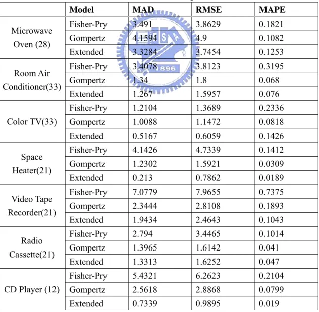
4.2 Predicted Performance between Models...55
4.2.1 The Test of Fisher-Pry Model and Gompertz Model ...55
4.2.2 The Test of Extended Logistic Model...57
4.2.3 Comparison between Models...58
4.3 A case of Technological Substitution in Digital Camera Industry ...62
4.4 Results of the Tested Hypotheses...63
CHAPTER 5 CONCLUSIONS ...65 5.1 Conclusions...65 5.2 Contributions...67 5.3 Research Limitation...68 5.4 Further Research ...69 REFERENCE...70 Appendices...73
Appendix 1: The Mathematical Inference of Fisher-Pry Model...73
Appendix 2: The Mathematical Inference of Gompertz Model...74
Appendix 3: The Penetration of Durable Goods in Japan ...76
Appendix 4: The Procedures of estimating parameters ...77
Appendix 5 The Process of Running the Gompertz Model...81
LIST OF TABLES
Table 2. 1 The comparison of technological forecasting methods...12
Table 2. 2 The map of technology forecasting methods. ...13
Table 2. 3 The recent researches using quantitative technological forecasting methods ...18
Table 3. 1 The classification of data sets ...32
Table 4. 1 Coefficients of Fisher-Pry and Gompertz Model...45
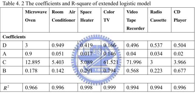
Table 4. 2 The coefficients and R-square of extended logistic model ...46
Table 4. 3 The comparison between long data sets...50
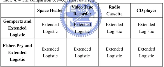
Table 4. 4 The comparison between short data sets...53
Table 4. 5 The rank of models in symmetric, asymmetric, and other data sets ...54
Table 4. 6 The criterion between models in durable goods. ...54
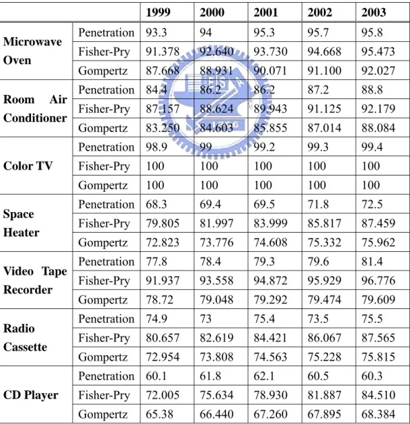
Table 4. 7 The penetration and prediction in last five points (Fisher-Pry and Gompertz). ...56
Table 4. 8 The penetration and prediction in last five points (Extended Logistic). ...58
Table 4. 9 The comparison between long data sets (Forecasts) ...59
Table 4. 10 The comparison between short data sets...59
Table 4. 11 The criteria between models in prediction part...60
Table 4. 12 The criteria between models in prediction part before point of inflection. ...61
Table 4. 13 The criteria between models in pixels (more than two million pixels)...62
Table 4. 14 The criteria between models in pixels (less than two million pixels)...62
Table 4. 15 The rank of Fisher-Pry and extended logistic model in performance ...64
LIST OF FIGURES
Figure 1. 1 The structure of thesis. ...7
Figure 2. 1 Steps in trend analysis ...14
Figure 2. 2 Classification of quantitative technological forecasting models ...16
Figure 2. 3 The process before model fitting...17
Figure 2. 4 The S-Curve...20
Figure 2. 5 The point of inflection in S-curve. ...21
Figure 2. 6 Comparison of exponential and logistic...23
Figure 2. 7 Life cycle phases ...24
Figure 2. 8 The typical obsolescence and S-curve chart...25
Figure 3. 1 The process of research ...30
Figure 3. 2 The penetration of durable goods in Japan...31
Figure 3. 3. The percentage of pixel-change of Digital Camera...32
Figure 3. 4 The point of inflection of Fisher Pry ...35
Figure 3. 5 The point of inflection of Gompertz...38
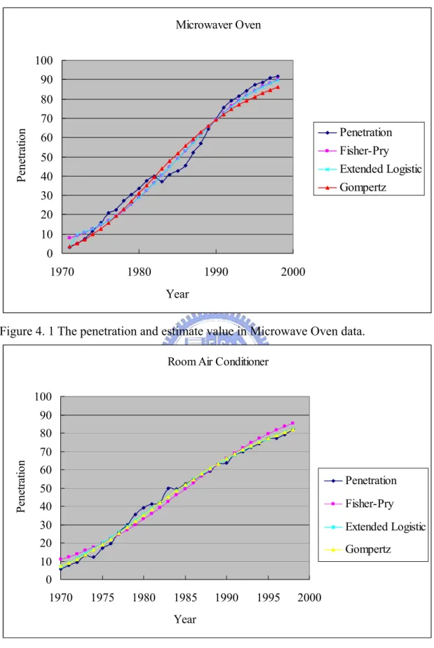
Figure 4. 1 The penetration and estimate value in Microwaver Oven data. 48 Figure 4. 2 The penetration and estimate value in Room air conditioner data. ...48
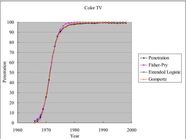
Figure 4. 3 The penetration and estimate value in Color TV data. ...49
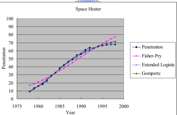
Figure 4. 4 The penetration and estimate value in Space heater data. ...50
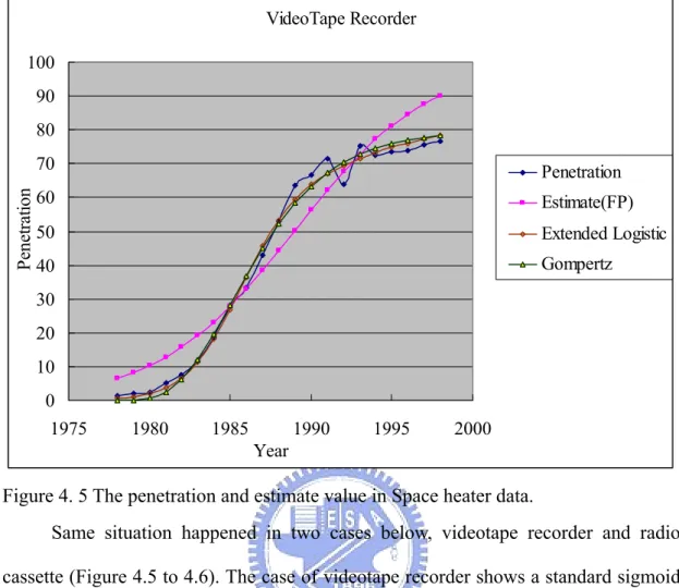
Figure 4. 5 The penetration and estimate value in Space heater data. ...51
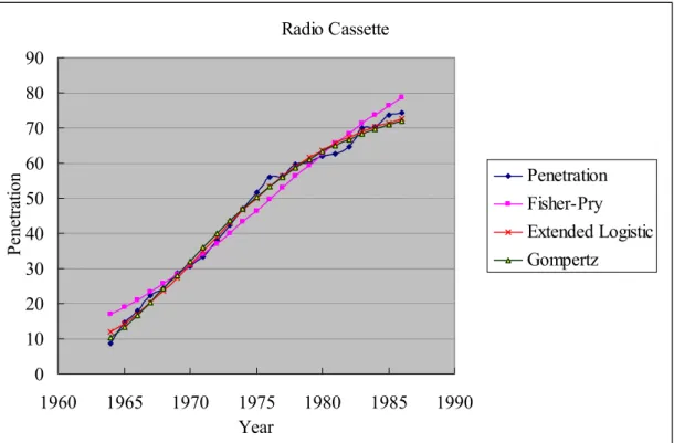
Figure 4. 6 The penetration and estimate value in Radio Cassette data. ...52
CHAPTER 1 INTRODUCTION
Technology forecasting has been developed for several decades, and some of methods were derived from other field such as demography. For example, the trend of the adoption of a product will grow slowly at first, and then it will have rapidly growth. Finally, the growth of the adoptions will look like a sigmoid curve. Some quantitative technology forecasting model, such as Fisher-Pry and Gompertz, can offer a precursor when a new product replaces a mature product, and they can offer the probable trend of the market share of a new product. This chapter first presents a brief background to the technology forecasting, and then the problem discussion will be introduced. The research purpose and motivation are also presented with the overall structure of this research in this chapter.
1.1 Background
Technology forecasting has been developing during several decades and is still in the process of improving since many new technological inventions increases the demands of forecasting tools. Many enterprises need these methods in their focus field in order to improve their projection ability and to know the trend as many as possible. Some consultative companies also use technology forecasting method to offer the projection about some products or technologies. Therefore, technology forecasting is comprehensively used now. The technology forecasting can simply divided into two fields according to quantitative or qualitative way. However, these methods truly offer an auxiliary role when managers need to make a decision whether they use quantitative or qualitative method.
bell-shaped curve, and this curve can be divided into five parts- Innovators, Tornado, Main Street, Decline, and Obsolescence. As same as the life cycle, technology adoption life cycle can also fall into five parts- innovators, early majority, late majority, and laggards (Meade and Rabelo, 2004). Therefore, the growth of adopters in new products or services will look like a sigmoid curve, and they will also decline as sigmoid way. Some technology forecasting methods can be a tool to fit and forecast this trend, such as Fisher-Pry and Gompertz. However, there are many adapted or new models proposed in this field (Carrillo and Gonzalez 2002, Bhargava 1995, Rai and Kumar 2003). These methods can fit data sets well in some specific products or services, such as the rate of adoption of mobile phone, and it portrayed the trend of a new product or a service.
1.2 Problem Discussion
Technological forecasting models give the projection and fit in the form of graph according to estimation of points during a period. The forecasters first may observe the market share or sales volumes data, and the time measures can be annual or quarterly. Although many adapted or new technological growth curve models which used to fit the data were proposed in recent years, not every model can fit or forecast well in different kinds of data sets. Technological forecasting models can be classified according their characteristics (e.g. symmetric, asymmetric, and flexible), the method of estimation, and so on. These classification may offer a simply and clearly way to identify which model belongs to which categories. Consequently, some researchers try to find some criteria to identify which model will have better fit or forecast performance in some particular data sets (Young 1993, Meade and Islam 1997). These classifications can reduce the biases which technological growth models made. For example, the symmetric sigmoid curve can be fitted well by symmetrical
technological growth model (e.g. Fisher-Pry). However, there are more implications for model selection. Choosing the right model is an important work before researchers prepare to project the time series data points. Some models perform a better forecast but fail to forecast the short term time-series data. Another way to reduce the bias is to use the combined models, and this method will also help the forecasters reducing the error when they did not use an appropriate model to fit the data (Meade and Islam, 1997).
Some growth curve may not reach the saturation level at 100%, because the new technologies may enter the market and adopt the share of the mature one before the mature product reach the saturation at 100%. This phenomenon may make some technological growth models (e.g. Fisher-Pry) can not fit these data well. Therefore, when the limit of capacity is unknown, some models will not fit or forecast well in this situation. Experts’ opinion seems a good method to solve this problem if experts suggest a proper limit of capacity. However, if a model can be adjusted its capacity with time-varying, the prediction of limit of capacity can be ignored. Moreover, the number of observations will affect the forecasting accuracy. The more observation points can be obtained, the more accuracy of the curve can be estimated. The stable and robust estimation can be obtained if the data includes the peak of noncumulative adoption curve (Mahajan, et al. 1998).
There are some generalized, adapted, or new technological forecasting models proposed in recent years. The generalized and adapted models are based on the prior common models, such as Fisher-Pry and Gompertz, and adapted them through estimative methods, number of parameters, and so on. Moreover, the saturation level (or called capacity) is limited or not also affect models drawing the fit or predicted performance. There is an interesting idea about the capacity of logistic model, which proposed by Meyer and Ausubel (1999). They argued that the capacity of logistic
curve will also vary during time. This research will try to find whether a dynamic capacity will help the model have better performance.
According to the discussion about the technological forecasting model in this section before, some research directions can be found. First, this model will also have a flexible inflection point in order to fit different kinds of data sets. That can improves that one model is suitable for some data sets whether they belong to symmetric or asymmetric form. Second, dynamic saturation level will help researcher save the process to find the possible saturation level. Finally, the number of data will affect the outcome of forecasts.
1.3 Research Motivation
The growth of a product or a service is interesting process, because its shape looks like a sigmoid curve as similar as the growth of population. Therefore, some methods which used in demographic field were comprehensively used in fitting or projecting the technological growth. These methods are generally called the technological forecasting models or technological growth models. However, not all of data will follow the sigmoid curve. They may follow linear-like or other forms. Although there are so many technological growth models can be used in fitting different kind of data sets, some improvements can be found in these models and try to find a better method to fit the data. That is why so many adapted or new models were proposed in decades.
The growth of a product or a new service may not easily be observed when only few data can be gathered, but the similar growth trend may also be happened in mature products. For example, people used canals, railways, road, and airways to be the transportation way, and then the growth of maglev may be seen as similar as these mature technologies (Meyer et al., 1999). Therefore, the fit of a growth model not
only can find the trend of data, but also offer a possible way which a new product or service is followed. Moreover, the growth curve can offer some useful information in managerial information. For example, the point of inflection can provide when the products will reach the maximum rate of penetration, and when the curve will reach the saturation level roughly.
1.4 Research Purpose
The growth curve can offer some useful information in managerial information. For example, the point of inflection can provide when the products will reach the maximum rate of penetration, and when the curve will reach the saturation level roughly. There are many quantitative technological forecasting models in this field, and many generalized form were also proposed (Bhargava1995; Rai and Kumar 2003) in order to improve the forecast. Therefore, the way to utilize these models in the right case is more important nowadays in order to get the better fit and forecasting performance, and some scholars have proposed some related paper about the model comparison and selecting criterion (Young 1993, Meade and Islam 1997). Although so many technological forecasting models were proposed, less of them can be used to forecast extensively. The articles proposed about new or modified models explain for a particular time-series data (Young, 1993).
Although there are so many new or adapted models have been proposed in recent decades, some improvements are still can be found in these models. The main purpose of this research will try to find a new technological forecasting model according to the time-varying capacity called the generalized logistic model, and make several comparisons between the extended logistic model and Fisher-Pry model, which is most commonly used in quantitative technological forecasting. Moreover, the comparison will be based on the length of data, and the shape of data.
This thesis will try to find a proper model which capacity growth with time-varying and make a comparison between a new extended logistic model, Fisher-Pry model, and Gompertz model. The goal of this research is to identify the extended logistical model will have a better fit and forecast than Fisher-Pry model and Gompertz model, which are comprehensively used in related area. This research will use the different kind of data sets to test these three models, and data sets will be simply classified in order to identify the performance of these two models in different classification.
1.5 Research Content
The scope of thesis can be divided into several parts, and the basic outline of this thesis was shown (Figure 1). The introduction offers the overview of thesis and the outcome roughly, and talks about the purpose of this research. The literature review gives some definitions such as technology forecasting, technology substitution, the life cycle, and so on. The data collecting will describe why this research collects these data sets and then analyze the outcome of the test in these two models. After analyzing, comparing between these two models will be implemented and set the conclusion.
Figure 1. 1 The structure of thesis. Introduction, Research
purpose and motivation
Literature review
The definitions and methods of technology forecasting
Comparison between models and Result
Data collection and Analyses
The trend of durable goods in Japan Conclusion and
CHAPTER 2 LITERATURE REVIEW
This chapter will introduce some prior researches and some definition related to technological forecasting. Some definitions related to technological forecasting will be introduced in detail, such as technology forecasting, adoption life cycle, and technological substitution. Then some details related to these parts will also be talked about. Finally, this chapter will show some applications of technological forecasting models which some authors proposed before and the selection criteria that prior researches made.
2.1 The Definition of Technology Forecasting
Before talking about the technology forecasting, the words, technology and forecasting, should define first. According to the definition of the American Heritage Dictionary of the English Language, the word “Technology” is the application of science, especially to industrial or commercial objectives, or the scientific method and material used to achieve a commercial or industrial objective. The other word, forecasting, is to estimate or calculate in advance, especially to predict by analysis of meteorological data or to serve as an advance indication of; foreshadow: price increases that forecast inflation.
The definitions of technology and forecasting are described at last section, and some description of technology forecasting will be discussed. Technology grows up sharply in the decade of the end of 21 century, and it is important to project the next new generation products or to see the technology substitution. Technology forecasting can be defined as a prediction of the future characteristics of useful machines, procedures, or technologies. (Martino, 1993) Forecasting is intended to bring the
information to the technology management process and to try to predict possible future state of technology or conditions that affect its contribution to corporate goal, so the technology forecasting might be requested to determine what computation power will be on the manager’s desk in five or more ten years. However, the attributes of technology most often forecast are:
1. Growth in functional capability
2. Rate of replacement of an old technology by a newer one. 3. Market penetration
4. Diffusion
5. Likelihood and timing of technological breakthroughs.
Forecasters must know the characteristics of growth when they want to forecast the technology or diffusion. They also need to know the attributes of the technology to anticipate how the technology will be used and to choose the legal measures. These measures may be different in forecasting the technology. For example, when using the speed to be the measurement of the products, such as cars, it may not represent the growth in functional capability. Speed may just represent the one of the attributes of the cars. Therefore, choosing right measurement in right technological forecasting methods is important in technology forecasting field. (Porter, Roper, Mason, Rossini, Banks, 1991)
Although the concept and practice of technology forecasting has been proposed for more than three decades, there are two recent developments that have revitalized interest in it. The first of these developments is the enormous increased in the cost of conducting research and development, and the second is the integration of market consideration into technology forecasting process. Indeed, technology forecasts take this reality into consideration, and a major goal is to determine what advances in technology will result in increased sales, enhanced profits, and delighted customers.
(Vanston, 1996)
2.2 The Methods of Technological Forecasting
This section will introduce the classification of technological forecasting, and mainly describe the quantitative technological forecasting, including the type of models, model selection, and application.
2.2.1 The Classifications of Technological Forecasting
When we want to project the future of one industry, we have more than 150 technology forecasting techniques to choose. This section will introduce the classifications of the methods of technological forecasting. However, there are about 18-20 techniques used in various business and others for practical forecasting. Thus, Vanston (1996) thinks that forecasting technologies involve methods. First way is to identify, organize, and extrapolate patterns of past technical development. Second way is to gather and consolidate the opinions of people with special expertise in the areas to be forecast.
The methods of technological forecasting, in a word, can be divided into two simply groups, quantitative and qualitative. However, this classification which just likes dichotomy may not exactly interpret these technological forecasting models. Porter and Rossin (1987) suggested that the hundreds of technology forecasting methods can be categorized in five families, and Porter, Roper, Mason, Rossini, Banks (1991) summarized these methods in their assumptions, strengths, weaknesses, and uses.
1. Monitoring: It is the process of scanning the environment for information about the subject of projections, and this method just like a tool for gathering and organizing the information. The sources of information will be identified and
then information
2. Expert opinion: The opinion of experts in particular technology field are
gathered and analyzed. The assumption of this method is that some experts will know more in particular area than others, therefore the forecasts they projected will more accuracy than others.
3. Trend extrapolation: It uses mathematical or statistical technologies to extend time series data into future. This assumes that past conditions and trends will continue in the future.
4. Modeling: It represents some structures and dynamics of some parts of real
world, and it can be used to forecast the behavior of the system. Models can be flow diagrams, simple equations, and scale models to complicated computer simulations. It assumes that the basic structure and processes of parts of world can be captured by simplified representations.
5. Scenarios: It likes the overview of some aspects of the future leading from the present to the future, and it encompasses the possible range of possibilities for some prospects of the future. Scenarios assume that unable forecasts can be constructed from a narrow data base, and future possibilities can be reasonably incorporated in a set of imaginative descriptions.
Table 2. 1 The comparison of technological forecasting methods.
Strengths Weaknesses Uses
Monitoring Providing large useful
information. Information overload happened without selections. To provide useful information for structuring a forecast. Expert Opinion Tapping high-quality models internalized by experts Identifying experts is difficult and some extraneous factors will affect experts.
To forecast when experts in this field exists and where data are lacking. Trend Analysis A substantial and data-based forecast of quantifiable parameters.
It requires good and enough effective data and it did not explicitly address the causal mechanisms.
To project quantifiable parameters, and analyze adoption and substitutions of technologies.
Modeling Simplifying the future
behavior of complex systems. Building process provides good insight into complex system behavior.
Models that are not heavily data-based may be misleading.
To reduce the complex systems to manageable representations.
Scenarios It can portrait the
possible futures explicitly and incorporate qualitative and quantitative information produced by others.
It may be more fantasy than forecast, unless a firm basis in reality is maintained by the forecasters. To integrate quantitative and qualitative information and to integrate forecasts form various sources. To provide a forecast when data are too weak to use other methods.
Note: source from Forecasting and Management of Technology, Porter et al, Wiley Interscience.
Porter et al. (1991) categorized technology forecasting methods into three parts: 1. Direct: Direct forecasting of parameters that measure an aspect of technology. 2. Correlative: Correlative parameters that measure the technology with
3. Structural: Explicit consideration of cause-and –effect relationships that effect growth.
Many factors will affect the outcome we projected, so there are a lot of models proposed by many people and used in different kind of technology forecasting. Therefore, we can find some ways to view the future.
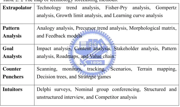
Vanston (2002) classified the technology methods into five categories, and point out what is quantitative or qualitative clearly (Table 2.2).
Table 2. 2 The map of technology forecasting methods.
Extrapolator Technology trend analysis, Fisher-Pry analysis, Gompertz
analysis, Growth limit analysis, and Learning curve analysis
Pattern Analysis
Analogy analysis, Precursor trend analysis, Morphological matrix, and Feedback models
Goal Analysts
Impact analysis, Content analysis, Stakeholder analysis, Pattern analysis, Roadmaps, and Value chain
Counter Punchers
Scanning, monitors, tracking, Scenarios, Terrain mapping, Decision trees, and Strategic games
Intuitors Delphi surveys, Nominal group conferencing, Structured and
unstructured interview, and Competitor analysis Note: Source from Technology futures, Inc.
2.2.2 Quantitative Technology Forecasting Methods
As last section has been mentioned, quantitative technology forecasting methods can be classified into extrapolators (Vanston, 2002) and trend extrapolators (Porter el al, 1991). It relies largely on direct time series analysis, and the valid data is necessary. Forecasters believe that the past data contains all the information to project the future (Martino, J.P., 2003). By this reason, forecasters think that the future will represent a
logical trend and will be projected by past data. Besides, quantitative technology forecasting methods should be used in conjunction with complementary technology forecasting methods, like expert opinion and monitors. (Porter, Roper, Mason, Rossini, Banks, 1991)
When the variables have been chosen and the necessary data have been obtained, trend analysis can begin. First we have to identify what model we should use, S-shaped growth curves, Learning curve, Exponential growth, or Linear. In the second stage, we have to fit the model to the data through graphical way and to solve for the parameters in the equation. In the third stage, we have to project the future possible situations graphically or mathematically. Finally, we have to compute the confidence intervals and to consider outside factor in order to interpret the projection and perform sensitivity analysis.
Figure 2. 1 Steps in trend analysis Identify the
proper model
Fit the model to the data
Use the model to project
Perform sensitivity analysis and interpret the projections
Martino (2002) also said that forecasting by extrapolation means that the forecaster assumes that the past of a time series contains all the information needed to forecast the future of that time series. That is why some quantitative technological forecasting methods just used time to be the variable, then forecast or fit the data (cumulative market share, penetration, or sales volume).
2.2.3 Type of Quantitative Technological Forecasting Methods
Models which used in technological forecasting can usually be classified
according to measurements, shape of curve, and the point of inflection. In prior research, these methods were investigated and found the classification of these methods. The common classification is based on shape, and this research classifies these models based on measurements and shape (Figure 2.2). When forecasters want to project the diffusion trend about a new product, they can use two kinds of measurements, proportion or units, according to what kind of data can be obtained. The Internal-influence model means that the rate of diffusion is viewed as a function of social interaction between prior adopters and potential adopters in the social system. The prior adopters can be seen as initial buyers and potential adopters can be seen as potential buyers. The behavior that initial buyers affect the potential buyers to buy a product can be treated as social interaction. Mix models combined the internal-influence model and external-influence model, which is affected by outside of social system. After deciding which measurement is decided to project, forecasters can choose internal-influence or mix model to be the forecasting tool (Mahajan and Peterson 1985, Frank 2002).
Models
Proportion Units
e.g. Penetration e.g. Cumulative adopters
Internal-Influence Models Mix Models
Symmetric
Figure 2. 2 Classification of quantitative technological forecasting models
2.2.4 The selection of technological forecasting models
Many kinds of technological growth curve model have been proposed in
decades. This section will describe the selection criteria about the technological growth models. These criteria are based on observing the characteristics of data sets, such as length of data, 50% takeover point, and upper limit. These characteristics can help forecasters know what kind of technological growth model that is appropriate to be the tool of projection. Young (1993) used nine technological growth models to test which one would perform better in different kinds of data sets. He set some criteria about choosing the models in different kinds of data sets. Therefore, he offered selecting criteria before fitting data sets, and this can help the forecasters avoid biases
e.g. logistic Nonsymmetric e.g. Gompertz Flexible Fixed e.g. Bass Flexible e.g. NUI e.g. NSRL
before model fitting and projecting. The process before model fitting will be shown in this section (Figure 2.3). First step is to identify the characteristics of data sets. Then forecasters can choose one or several appropriate models according to the characteristics of data sets.
Length of data sets
Figure 2. 3 The process before model fitting
Source: From “Technological Growth Curve: A Competition of Forecasting Models”, 1993.
2.2.5 Applications of technological forecasting
Technological forecasting methods are commonly used in lots of area, such as
the trend of technological growth, and technological substitution. In prior research, wireless communications are popularly investigated through technological forecasting methods. Some of these researches used the penetration to be the measurement (Vanston, 2002), and others used the units (e.g. subscribers) to be the measurement (Frank, 2004). Not only one but also two or more models were used in these researches (Table 2.3). The research subjects of these prior papers do not only focus on a product or an industry, but also investigate into a service. Therefore, quantitative
Data sets Knowledge of upper limit
50% takeover point
Choosing appropriate models
technological forecasting methods are suitable for different kinds of industries, products, and services.
Table 2. 3 The recent researches using quantitative technological forecasting methods
Author Measurement Method Object
Frank (2004) units Modified Logistic Wireless Communications Hodge (1998) units/percentage Fisher-Pry/Gompertz Analog and Digital
Cellular Phone Rai and Kumar
(2004) percentage Fisher-Pry/ Rai’s Model Color TV, Railway, and Thermal electricity Palmer and
Williams(1999) units Fisher-Pry Electronic Industry
Victor and Ausubel
(2002) units
Logistic/Fisher-Pry
transform DRAMs
Vanston (2002) percentage Fisher-Pry/Gompertz Residual Broadband
2.3 The Growth Curve
This section will talk about the growth curve, which is commonly used in interpreting the trend of a product, an industry or a service. First part will interpret the definition of growth curve. Then the representative form of growth curve will also be introduced. Finally, the adoption of life cycle which is similar to product life cycle will also be presented in this section.
2.3.1 The Definition of Growth Curve
Every product or service has its own growth curve, and every growth curve may roughly look similar but different in detail. These growth curves may appear in a wide variety, such as parabolic, power, exponential, sigmoid, and so on. Some researchers investigated these phenomena and demonstrated the growth may show not only sigmoid curve but also other forms (Rai and Kumar 2003, Porter et al 1991). However, the most commonly growth curve is sigmoid curve (S-curve). The S-Curve is the well-known concept in the innovation management, and this concept is also applied in interpreting the trend of one technology. The technical progress or performance of products basically follows sigmoid shape of performance versus time, and the measurement can be a product life cycle, a technological life cycle, or some economic performance or technical parameters. Consequently, the S-curve plays an important role in technology forecasting, because it can roughly describes the trend of technology forecasting by a graph. There are many strong evidences that in many cases, the diffusion of technologies demonstrated that it follows the smooth growth pattern just like the S-shaped. For example, Palmer and Williams (1999) employed the Fisher-Pry model to fit the microprocessor clock speed. Hodges (1998) used Fisher-Pry and Gompertz model to fit the analog and digital cellular, and he found that the trend roughly obey the S-shaped curve.
The S-curve shows the revolution of technology and it can be divided into three phases of performance (Figure 2.4). In the first phase of introduction, the new technology may just be developed, and there are still a lot of problems such as financing, process of production, unfamiliar, imperfect and so on. Therefore, the growth of first stage rises slowly and gently. In the second phase of rapid adoption, the new technology has been achieved the economies of scale, and people learn more
about the new technology. Besides, the new technology improves and finds more applications. Therefore, the trend of this stage rises sharply in market share. Finally, the third phase of saturation seems to rise more gently than phase 2. The development of technology in this phase may meet the bottleneck, and some new technology may grow stronger and overtake the market share of old technology. In another word, this technology is mature.
Figure 2. 4 The S-Curve
Limit of Performance
Performance
Parameter
Phase 1 Phase 2 Phase 3
Saturation
Introduction
Rapid Adoption
Time
Source: From “Development of a Methodological Framework for Examining Science and Technology in Flanders,” 2000.
The point of inflection is an important characteristic of growth curve (Figure 2.5). It happens when the rate of change reached the maximum value. The point of inflection can be used to judge the growth curve is symmetric or not. In general, the maximum rate of change symmetric curve (e.g. Logistic) is a constant that occurs when 50% of potential adopters have adopted the product. However, the nonsymmetrical curve, such as Gompertz, can also be calculated its point of inflection.
For example, the percentage which the point of inflection reached is about 37%. That means the point of inflection in Gompertz will happen before 50%. Flexible models, which have flexible point of inflection, will reach the maximum rate of change when equal or less than 50%.
Figure 2. 5 The point of inflection in S-curve.
dF (t)/dt
F(t)
t t
t* t*
2.3.2 The Representative of Growth Curve
Some different kinds of growth shape have been mentioned briefly in last section, and some representatives of growth curves will be introduced now. The growth curve is based on calculating the cumulative sales, penetrations, or key performance parameter. For example, calculating the proportion of cumulative adopters who have adopted a product can draw the shape of growth curve. Consequently, here are some questions about the growth curve. What kind of curve may the growth of technology be? Is it an exponential, sigmoid, or other curve? The most commonly curves are exponential and sigmoid, and there are some comparisons of two curves in the underlying section.
The growth of population or technology may shows the exponential growth, but they wouldn’t always grow up rapidly (Equation 1). If a negative feedback term is added to this equation, some restrained effect will turn the exponential growth curve into sigmoid curve.
t
e
t
p
(
)
=
β
α (1) The most widely used modification of exponential growth is logistic. Adding a negative term will make exponential growth transferring to logistic growth (Equation 2). The feedback term is near to zero when P (t) → k and near to 1 when P(t)<<k. Therefore, solving the differential equation can get the solution by integrating, and the solution will be similar to S-shaped curve (Equation 3).⎟
⎠
⎞
⎜
⎝
⎛ −
=
k
t
P
t
P
dt
t
dP
(
)
1
)
(
)
(
α
(2)(
( ))
exp 1 ) ( b t k t P − − + =α
(3)When putting a feedback term to the exponential function, some inhibitions will be revealed. The new equation belongs in the technology growth or other field such as population growth. Every technology can’t grow infinitely and show a development like the exponential curve. Consequently, it has its limitation in market share, just like the life cycle of technology. The half of life cycle can be divided into three phase; Introduction, Rapid adoption, and Saturation. The logistic function can fit better than exponential function in technology forecasting (Figure 2.6).
Exponential
Logistic
Time Figure 2. 6 Comparison of exponential and logistic
2.3.3 Technology Adoption Life Cycle
When one new product is thrown into the market, it may success or fails in market. Same as one new technology is proposed. Therefore, the technology adoption life cycle can show what place the technology or product is in. It classifies the market and the reactions to a high-tech product. The technology adoption life cycle is the tool for determining the products, pricing and marketing strategies for high-tech products, and was defined as consisting of six phases, including innovation, chasm, tornado, Main Street, decline and obsolescence.
The phases and the trend of life cycle can be shown (Figure 2.7). The phase of chasm means that it goes down in phase 1. Consequently, some new technology may fall into this phase and can be judged that it may not go to the phase of Main Street. (Meade, P.T., Rabelo, L., 2004)
and decline. In the first phase, the new technology has to compete with other technologies. In the saturation stage, all technologies have competed, and the growth of new technology faces the limit. In the last phase, no competition will be concerned.
Market
Share Main Street
Tornado Decline
Chasm
Obsolescence Innovators
Time
Figure 2. 7 Life cycle phases
Note. From “The technology adoption life cycle attractor: Understanding the dynamics of high-tech markets,” by Meade, P.T., Rabelo, L., 2004, Technology Forecasting & Social Change, 71, p.670.
2.3.4 Technological Obsolescence
Obsolescence can be thought simply as the assets loss in value when the market expectation is increasing, the utility of assets is still the same. For example, when the utility of notebook increase, such as wireless function and power saving, the consumer’s expectation will also increase. Then the old generation notebook will lose its value gradually in that the consumers’ need increases.
The technology S-curve was introduced in the last section. Consequently, technological obsolescence will happen following with the technology change, and
this phenomenon can be observed by using technological substitution analysis, such as Fisher-Pry model, which based on the adoption of potential adopters. The old technology has economics of scale, and it is well known and mature in the first stage. Basically, the appearance of obsolescence is not very clear in old technology at early stage when a new technology entries in the market. However, when new technology grows up and achieves its economics of scale and has more improvements, the old technology can’t enhance its market share and start to follow a downward tendency. In the final stage, the old technology will decline to zero and be displaced by new technology (Figure 2.8).
Market Share
Market Share of
Figure 2. 8 The typical obsolescence and S-curve chart
Time Old Technology Market share of New Technology Saturation Rapid Adoption Introduction
2.4 Technological Substitution
Technological change is a dynamic and multidimensional phenomenon involving substitution and diffusion of technologies (Rai, A.P., Kumar, N., 2003). Technology substitution can be defined as a process by which an innovation is replaced partially or completely by another in terms of its market share or sales volumes over a period of time. This process follows the adoption life cycle and can be listed in several emphases.
z New technology enters the market and grows as a logistic curve (e.g. Fisher-Pry type for two competitors).
z Only one technology will reach the saturation level at any given time.
z A technology in saturation level will follow a non-logistic path and then will begin to decline which follows a reverse logistic form.
z A declining technology still follows a reverse logistic form (e.g. Reverse Fisher-Pry for two competitors) and becomes no competition gradually. (Meyer, Yung, and Ausubel, 1999)
For example, .Hodges (1998) investigated that the transfer of the subscribers between the analog and the digital systems in the U.S. was obeyed the technological substitution process. This process was fitted and projected by some technological substitution models (e.g. Fisher-Pry model). In general, we can use the mathematical methods to predict the trend of the technology substitution, and substitution models proposed by different researchers are based on the assumption that the replacement factor is a function of the market share captured by the technology (Rai and Kumar, 2003). Basically, fitting and projecting the substitution of technology is important, and it can let the enterprisers know how they should adjust their strategies and know the timing of launching a new product. However, Morris and Pratt (2001) said that
forecasting technological substitution requires a model that generates intuitive understanding of the factors affecting substitution but that also has good predictive ability.
2.5 Hypotheses
The development of technological forecasting is popularized in decades, and not only qualitative but also quantitative methods have been investigated comprehensively. This research focuses on one branch of quantitative technology forecasting model that based on estimating the penetration or the market share of a product. This research proposes a new model based on a dynamic capacity, and use this new model to compare with Fisher-Pry model and Gompertz model.
The derived literatures proved that put a right technological forecasting model into an appropriate data set will increase the accuracy of fit performance. There are two commonly technological forecasting models, Fisher-Pry and Gompertz, and these two models can fit well in symmetric (e.g. Fisher-Pry) and asymmetric (e.g. Gompertz) data sets. However, not all the products or technologies will grows as symmetric sigmoid curve. This research will test the Fisher-Pry model and Gompertz model in some data sets which grows not only as symmetric but also asymmetric and other forms, and the extended logistic will also be examined in same condition. In order to examine whether Fisher-Pry, Gompertz or extended logistic model can offer a better fit performance, the hypothesis will be set as below:
H1: The extended logistic model will have a better fitting performance than Fisher Pry model and Gompertz model in both long and short data sets.
The characteristics of growth curve of each data set may have influence on fitting performance when a technology forecasting model is used to fit the data set. According to prior researches about quantitative technological forecasting, Fisher-Pry
model offer a good fit in data sets which grows as symmetric, and Gompertz model can offer a better fit in asymmetric data sets. On the other hand, the new model, extended logistic, is supposed that it can offer a good fitting performance whether the data set is symmetric or not. Therefore, the hypotheses will be listed as below:
H2: The extended logistic model has better fit performance in symmetric, asymmetric, and flexible data set than Fisher-Pry model and Gompertz model. According the prior research, many research papers draw some data sets before checking the fitting performance to examine the predicted performance. The predicted performance of a data set is more important than fitting performance of a data set. The good fit of growth curve only can observe the trend of products or technologies in specified time period, but a good forecast can offer an omen of the adoption of new products. This research will test whether a good fit can product a good forecast and this will be put into the hypotheses. Moreover, the data which are drawn form different kind of data will used to examine the predicted performance in Fisher-Pry model and extended logistic model.
H3: The extended logistic model has better predicted performance in both long and short data set than Fisher-Pry model and Gompertz model.
If Fisher-Pry model can offer a good fit in symmetric data, it may also offer a good predicted performance in symmetric data, and so does Gompertz model. The extended logistical model will also be tested whether it can offer a good predicted in symmetric data. The other characteristic of data set, such as asymmetric data, will also be discussed in this research. Therefore, the comparison between these models will be hypothesized in this research.
H4: The extended logistic model has better predicted performance in symmetric, asymmetric, and flexible data set than Fisher-Pry model and Gompertz model. H5: A good fit performance will lead a good predicted performance.
CHAPTER 3 METHODOLOGY
This chapter will introduce the methodologies used in this thesis in detail. There are many quantitative models proposed using in technology forecasting area. Some of them are statistical models, and others are time-related models. Besides, an adapted way to improve the fit in technological forecasting models will be introduced in this chapter.
There are many forecasting methods in technology forecasting field, and some criteria can make sure of which one is better. First, matching the model to the fundamental phenomena can make researchers knowing what extent can be represented in the actual area. Second, it is important to tailor and select models to the horizon. Finally, some time-series related models should be found forecast validity in order to improve forecast more accuracy. (Armstrong, J.C., 2001)
This thesis will use some quantitative models and compare with these models in the penetration of durable goods in Japan, and test the technological substitution of the pixels of Digital Camera of Taiwan. Furthermore, the research structure and the introduction of data collecting will be introduced in this chapter.
3.1 Research Structure
The figure 4.1 shows the process of research structure in this thesis. In the first step, some proper methods will be chosen and one combined model which built by combining some proper models will also be proposed. According to the combining models proposed by Meade and Islam (1997), they classified the technological forecasting model by two characteristics, the point of inflection and shape. Some existent technological forecasting models and a combining model will be adopted in
this research. Then some data will be collected and put these data into the models to fit them. The process will be followed to draw the trend and project it. In this part, three different kinds of software can offer the forecasting tools to fit and draw the data.
However, comparing with models can extrapolate which one is better. Some criteria can be used to make the judgments. Furthermore, we can observe the level of fit by viewing the visible figure of trend in these growth curves.
Figure 3. 1 The process of research
Obtain the data Identify and create
the proper models
Fit the models to the data
3.2 Data Collection
The quantitative technology forecasting models need data like sales volumes, market share, and some other secondary data (e.g. Annual survey by statistical bureau). Finding the correct data is important to project the data more accuracy. Therefore, data can be collected by some authorities and government organizations, such as IT IS, MIC (Market Intelligence Center), DGBAS (Directorate-General of Budget, Accounting, and Statistics), and some other statistical bureau in other countries. This research will use the penetration of durable goods in Japan which were gathered from the Statistics Bureau of Japan, and test the technological substitution of digital camera which collected from MIC annual report.
Draw the trend and project the future
Interpret the result
In order to examine the fits of models, some penetrations of durable goods in Japan is used in this research, such as Microwave ovens, space heater, room air conditioner, color TV sets, videotape recorder, radio cassette, and CD player. These data sets will be divided into two parts. One is used to test the fit performance of models, and the other is used to test the accuracy of forecasts. Therefore, every data set will be retained last 5 data in order to test the accuracy.
Penetration of durables in Japan
0
20
40
60
80
100
1960
1980
2000
Year
P
en
etr
atio
n
Microwave ovens Space heaterRoom Air Conditioner Color TV sets
Video Tape Recorder Radio Cassette CD Player
Figure 3. 2 The penetration of durable goods in Japan
(Source: These data sets were gathered from the Statistics Bureau of Japan. http://www.stat.go.jp/)
These seven data sets can be classified according to the length of data, the point of inflection, and the knowledge of upper limit (Table 3.1). First, this research considers that a data set can be thought as long data if the number of observations is more than 25 in a data. Second, the type of graph can be roughly considered symmetric, asymmetric, or other forms. Finally, this thesis considers whether the graph reach the 100% level or not.
Table 3. 1 The classification of data sets
Long data sets Short data sets
Length of data sets
Microwaver Oven, Room Air Conditioner, and
Color TV
Space Heater, Video Tape Recorder, Radio Cassette, and
CD Player
Asymmetric Symmetric Other
The point of inflection Color TV, and Video Tape Recorder Microwaver Oven, and Room Air
Conditioner
Space Heater, Radio Cassette, and CD Player 100% Less than 100% Upper Limit Microwaver Oven, Room Air Conditioner, and Color TV
Space Heater, Radio Cassette, Video Tape Recorder, and CD
Player
Digital Camera grows rapidly in recent years, especially in technological growth in pixels. Data was collected from MIC annual electronic industrial report. This research simply divided the data into two groups, less than two million pixels, and more than two million pixels. The purpose of this classification is to test the trend of technological substitution between the old and new generation.
Digital Camera 0 10 20 30 40 50 60 70 80 90 100 0 2 4 6 8 10 12 14 16 Time Pe rcen ta ge
Less than 2 million pixels
More than 2 million pixels
3.3 Fisher-Pry Model
In 1971 Fisher and Pry published a paper that described a simple model of technological change. This model is equivalent to biological growth model, because the technological growth is similar to biological growth. Therefore, this model is a common model in projecting the technological substitution, such as the rate at which one technology will replace another. This model is based on the observation that most growth trends follow an “S-shape” curve or “logistic”, in time with an exponential growth rate in the early years.
Williams, Palmer, and Hughes (1999) mentioned that using this model can be justified on three assumptions:
z Many technological advances can be considered as a competitive substitution, a superior method take the place of an inferior method.
z If the market share of an older technology has progressed as far as a few percent, it will proceed to completion and new technology will reach the saturation level. z The fraction rate of substitution of new for old is proportional to the remaining
amount of old to be substituted.
It is convenient to take the fraction of potential market penetration, f, as the dependent variable where f = Y/L and L is the upper bound for the growth of the variable Y. The f value is between 0 and 1, and variable y can be the sales volumes or the market share. Using the sales volumes as variables is a good assumption to project the future, because it was influenced by many factors, such as service, distribution, and so on. Consequently, the rate of sales volumes can reflect the trend appropriately when the quantitative technology forecasting model is used.
3.3.1 The Mathematical Inference of Fisher-Pry Model
The mathematical inference will be discussed in this section, and the model will be explained by mathematical expression. Before discussing about the Fisher Pry model, the mathematical inference can start at the general idea of models for innovation diffusion. The process of mathematical inference about the Fisher Pry model will be shown in appendix 1. Therefore, this section will directly discuss the general inference of Fisher Pry model.
According to the Fisher Pry original model, the equation can formulate as:
(
(
1 df b f f dt = × −)
)
]
(4) The basic fundamental of this model is that the rate of change of f is proportional to both f and (1-f). The parameters, b, is effective to detect the interactive effort when the potential market share, (1-f), converted into accepting the new technology through the fraction, f, of the market share that accepted the new technology. Thus, we can use the integration to solve the f and get the common equation of Fisher Pry model. The function can be written by:[
0 1 1 exp ( ) f b t t = + − − (5) Raymond Peal proposed a forecasting model which is similar to Fisher Pry model, and it is called the Pearl curve. He utilized this model to forecast in demographic forecasting. Moreover, it can be used in examining the absolute growth of a technology rather than the fraction of market share that a technology was taken over by another technology. (Equation 3)1 1 exp( ) f c b = + − t (6) Fisher-Pry model also can be changed from the nonlinear form into the linear one. (Equation 4)Where f is the fraction of market share of the new technology, and
(1-f) is the fraction of the market share of the old technology; α is half the annual fractional growth in the early years, and is the time at which f =1/2. Fisher Pry is a symmetric model. That means its point of inflection will happen at f=0.5 (Figure 3.3). 0 t F 0.5F 0 t Time
Figure 3. 4 The point of inflection of Fisher Pry
Furthermore, the parameters in equation 3 can be calculated by the transformed Fisher-Pry linear model. This linear model is directed transformed by equation 3, and the parameters can be easily estimated. The OLS method used in linear regression can find the proper estimators in transformed Fisher-Pry model. (Equation 8)
(
)
(
0 ln 2 1 f t t f α ⎡ ⎤ = − ⎢ − ⎥ ⎣ ⎦)
(7) (1 ) ln f ln( ) Z c bt f − ⎡ ⎤ = ⎢ ⎥= ⎣ ⎦ − (8)3.3.2 The variants of Fisher-Pry model
The Fisher-Pry model can be modified to fit the trend; therefore, Bhargava (1995) proposed a generalized form of the Fisher-Pry model. He believe that the substitution rate, b, may not be always a constant; furthermore, he considered that the parameters b is a time dependent variable. B (t) is a time related function, and this function can has various forms. (Equation 9)
ln ( ) 1 f B t dt f ⎡ ⎤ = ⎢ − ⎥ ⎣ ⎦
∫
(9) Some possible forms can be express as equation 6, and we can solve the integration to some possible forms of generalized Fisher-Pry description.ln ( ) 1 c f a b t f ⎡ ⎤ = + ⎢ − ⎥ ⎣ ⎦ 2 ln 1 f a bt ct f ⎡ ⎤ = + + ⎢ − ⎥ ⎣ ⎦ ln 1 ct f a be f ⎡ ⎤ = + ⎢ − ⎥ ⎣ ⎦ (10)
3.4 Gompertz Model
The Gompertz model is occasionally referred to as a natality model and it is a little different from Fisher-Pry model, which is characterized as a growth model. When researchers want to use the Gompertz model in technology forecasting, some conditions that the equipment replacement is driven by equipment degeneration rather than technology innovation. The curve of Gompertz model represents an asymmetric form. Therefore, the Gompertz model can exhibit a good projection in technical performance, such as the speed of CPU or the storage of hard disk.
3.4.1 The mathematical Inference of Gompertz Model
This section will introduce and verify the Gompertz model. The mathematical inference can be started at the original form of Gompertz model. The original form can be expressed as:
( )
( )
(
L f f b dt df ln ln − × × =)
)
]
(11) An explicit mathematical inference of Gompertz model is shown in appendix 2, and this inference is proven by internal-influence model. After integrating the formulation (Equation 11), the equation of Gompertz model can be represented by:(
[
b ktf =exp− exp − (12)
where f= Y/L, and L is the upper bound for the number of units, y. The parameters b and k can be estimated from fitting the curve of the data. This equation is the variation of S-shaped curve, and so does Fisher-Pry. However, the Gompertz curve is not
symmetrical about the central inflation point, and its inflation point occurs at t= (ln b)/k. Gompertz model will reach the points of inflection before 0.5F, and this
can be the way to make sure that Gompertz model is a asymmetric model. As same as Fisher-Pry model, we can obtain the coefficient of parameters b and k by linear regression. The regression model can be showed by underlying equation:
( )
b kt f L Z ⎢⎣⎡ ⎟⎥⎦⎤= − ⎠ ⎞ ⎜ ⎝ ⎛ =ln ln ln (13)F
0
t
>0.5F
Figure 3. 5 The point of inflection of Gompertz
3.5 The Extended Logistic Model in This Research
The new growth model will be introduced in this research, and the mathematical inference will also be presented. In prior research, the technological forecasting models always based on this equation or its integration;
(
(
1 df b f f dt = × −)
)
(14) bt a f f + = ⎟⎟ ⎠ ⎞ ⎜⎜ ⎝ ⎛ − 1 ln (15) where is the constant and b in equations is still the same. aHowever, many variants based on growth model were proposed in last two decades (Bhargava 1995, Rai and Kumar 2003). Bhargava argued that the parameters may not always be a constant, and Rai and Kumar proposed several new models which changed the form of parameter, t, to be a logarithmic form or exponential form. Moreover, Meyer and Ausubel (1999) proposed a new thinking about the capacity of logistic curve. They considered that the capacity may also fluctuate according to time and grow as same as logistic curve (Equation 14).
( )
) 1 ( t k f bf dt df = − (16) where k( )
t is the function which is similar to logistic curve.Now the idea based on fluctuant capacity about the logistic curve will be introduced in this research. As the equation mentioned before (Equation 14), this research modified the equation as:
( )
t f(
a bt k f = + ⎟⎟ ⎠ ⎞ ⎜⎜ ⎝ ⎛ − ln)
(17) This research assumes thatk( )
t =1−D×exp(
−A×t)
, where the value of D can be anynumber and the value of A must bigger than zero. This research assumes that the capacity will fluctuate. A product may reach the saturation level at 80 or 60%, because the market share or substitution rate of this product may be affected by new products. It may not achieve the 100% of market share and may collapse earlier than expected.
3.5.1 The mathematical Inference of Extended Logistic Model in This Research
This section will be described the mathematical inference of the new model in order to make more clear about the new model. In last section, the adapted form of equation has been defined (Equation 14). The first step is using some mathematical calculation in order to cancel out the logarithm. Therefore, the exponential term is added in both sides of equation. Then the equation will become as:
( )
( )
(
bt a f f t k − × − = − exp exp)
)
(18) In order to simplify the equation, some algebraic expressions will be used. Let the letter, C, equals to , and put this transformation into the equation. After that, the equation can be expressed as:(
−a exp( )
(
bt C f f t k − = × − exp)
(19) Now the simplified equation has been demonstrated, and the next step is to findthe final equation. Therefore, this research will calculate the equation step by step and list the equation of every mathematical procedure. After doing a transformation to move the letter f in the denominator in the left side of equation, it becomes easier to find the final form of new model.
( )
t f f C( )
btk − = × ×exp − (20)
Finally, the final form of the model can be found through several calculations, and the equation can be solved. The equation,k
( )
t , can also be putted in the model. Therefore,two forms of new model can be expressed as:
( )
( )
bt C t k f − × + = exp 1 or(
)
(
Bt)
C At D f − × + − × − = exp 1 exp 1 (21)3.5.2 The Variants of Extended Logistic Model
There are many models related to the technological forecasting, and some models can be treated as the variants of other models. For example, Bertalanffy model can be expressed as:
( )
(
1 exp)
1α 1 bt c f − × + = (22) This model can be transformed into some common technological forecasting models. It gives the Fisher-Pry model whenα =1, and it becomes the Gompertz model asα →0. Therefore, the new model also can be taken as some variants of other models. The new model is similar to Fisher-Pry model when , and it becomes the extended logistic model (Mahajan and Peterson, 1978) as D=1 and A=B. Consequently, the new model can also be taken as the variants of other models.0 →