國 立 交 通 大 學
電信工程學系碩士班
碩士論文
高頻寬效率 OFDM 系統之通道估計與等化
Channel Estimation and Equalization for
Bandwidth-Efficient OFDM system in Time
Variant Channel
研 究 生: 陳俊勝
指導教授: 謝世福博士
高頻寬效率 OFDM 系統之通道估計與等化
Channel Estimation and Equalization for
Bandwidth-Efficient OFDM System in Time
Variant Channel
研 究 生:陳俊勝 Student:J. S. Chen
指導教授:謝世福 博士 Advisor:Dr. S.F. Hsieh
國立交通大學
電信工程學系碩士班
碩士論文
A Thesis
Submitted to Department of Communication Engineering
College of Electrical Engineering and Computer Science
National Chiao Tung University
In Partial Fulfillment of the Requirements
For the Degree of
Master of Science
In
Electrical Engineering
July, 2004
Hsinchu, Taiwan, Republic of China
中華民國九十三年七月
高 頻 寬 效 率 O F D M 系 統
之 通 道 估 計 與 等 化
學 生 :陳 俊 勝 指 導 教 授 :謝 世 福
國 立 交 通 大 學 電 信 工 程 學 系 碩 士 班
摘 要
在 有 限 頻 ? 下 , 增 加 頻 ? 使 用 效 率 是 重 要 的 事 情 。 為 了 消 除 IBI 和 ICI , 傳 統 的 正 交 分 頻 多 工 調 變 系 統 需 要 使 用 護 衛 間 隔 (GI),這 會 使 得 頻 寬 使 用 效 率 降 低。 在 本 論 文 中, 我 們 採 用 高 頻 寬 效 率 的 正 交 分 頻 多 工 調 變 系 統。 並 且 提 出 通 道 追 蹤 架 構,它 可 以 在 時 變 通 道 中 做 通 道 估 計 。 這 個 架 構 的 表 現 是 比 適 應 性 等 化 器 來 得 好 ,但 演 算 法 的 複 雜 度 是 比 較 高 的。為 了 解 決 追 ? 速 度 不 夠 快 的 問 題,我 們 提 出 了 平 衡 收 斂 步 伐 控 制 方 法。這 方 法 將 有 助 於 通 道 追 蹤 架 構 獲 得 更 好 的 均 方 誤 差 (MSE)。 在 電 腦 模 擬 中 將 會 證 實 我 們 的 推 導 以 及 提 出 的 方 法 。Channel Estimation and Equalization for
Bandwidth-Efficient OFDM System in Time
Variant Channel
Student: J. S. Chen Advisor: S. F. Hsieh
Department of Communication Engineering
National Chiao Tung University
Abstract
Conventional OFDM system needs a guard interval to cancel IBI and ICI. But, efficiency of bandwidth usage will be reduced. In this thesis, we adopt the bandwidth-efficient OFDM (BE-OFDM) system, which can adjust efficiency of bandwidth usage. A channel tracking structure is proposed for channel estimation in time variant channel. Its performance is better than the adaptive equalizer, but its all structure is more complex. To solve the slow tracking problem, we propose an balanced step-size control adaptive method with improved mean square error. Finally, our derivations and proposed methods will be validated in computer simulations.
Acknowledgement
I would like to express my deepest gratitude to Dr. S. F. Hsieh for his enthus iastic guidance and great patient. I also wish to thank my friends for their concern and help. Finally, I would like to thank my parents, family about their consideration and encouragement.
Contents
Chinese Abstract i
English Abstract ii
Acknowledgment iii
List of Tables vii
List of Figures viii
1 Introduction 1
2 Bandwidth-Efficient OFDM system model 4
2.1 Conventional OFDM system model… … … ....4
2.2 Bandwidth-Efficient OFDM system model… … … ..6
2.3 Efficiency of bandwidth usage...… … … 11
2.4 Comparison of conventional OFDM and BE-OFDM.… … … ...13
3 Channel equalizer and Channel estimation 14
3.1 Channel equalizer… … … ...15
3.1.1 One-tap equalizer… … … ..15
3.1.2 One Block equalizer… … … ..16
3.1.3 Reduced one block DFE complexity… … … … .… … … ....18
3.2.1 Signal model in training...19
3.2.2 Training: MMSE channel estimation… … … … .… … … ...20
3.3 Adaptive equalizer… … … ..21
3.3.1 LMS adaptive equalizer… … … 22
3.3.2 RLS adaptive equalizer… … … .24
3.3.3 Summary of adaptive equalizer… … … ...26
3.4 Channel tracking in BE-OFFDM system… … … ...27
3.4.1 LMS channel tracking… … … ...28
3.4.2 RLS channel tracking… … … 30
3.4.3 Summary of structures of channel tracking… … … ...32
3.4.4 Improved LMS channel tracking with balanced step-size… … … 33
3.5 Complexity of adaptive equalizer and adaptive channel tracking… … … ..35
4 Computer Simulation 37
4.1 Simulation environnent… ...… .… … … .… .37
4.2 Reduced factor of complexity for BE-OFDM system… … … ....40
4.3 Comparison of adaptive equalizer and adaptive channel tracking… … … .44
4.3.1 LMS algorithm… … … ...45
4.3.2 RLS algorithm… … … ...46
4.3.3 Summary of adaptive equalizer and adaptive channel tracking… … … … 48
4.4 Parameters of channel tracking… … … ..49
4.4.1 Effects of training length… … … ...49
4.4.2 Effect of time variant of channel… … … ...53
4.4.3 Efficiency of bandwidth usage … … … .55
Appendix 65
List of Table
2.1 Comparison of conventional OFDM and BE-OFDM systems… … … ..… … 13
3.1 Computation procedures of LMS adaptive equalizer… … … ...… … ..27
3.2 Computation procedures of RLS adaptive equalizer… … … ..27
3.3 Computation procedures of LMS channel tracking… … … .… … ..33
3.4 Computation procedures of RLS channel tracking… … … ..… … ..33
3.5 Compared complexity of adaptive equalizer and channel tracking structure… … 36
4.1 Efficiency of bandwidth usage setting, Ω=2… … … .… .41
4.2 Efficiency of bandwidth usage setting, Ω=1.5… … … ..… .42
List of Figures
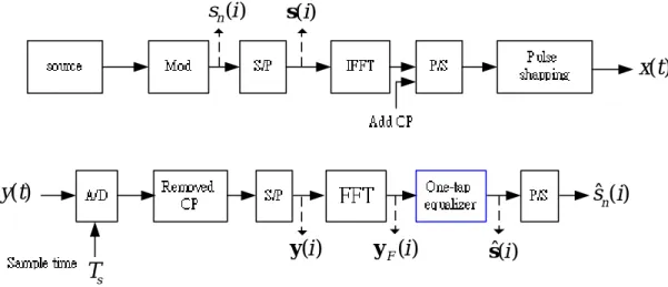
2.1 Conventional OFDM system… … … ..… … ..5
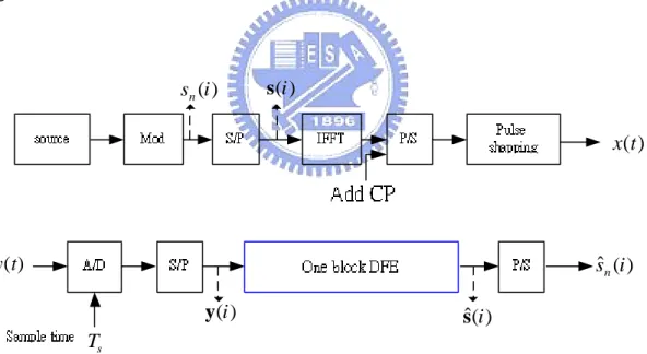
2.2 Bandwidth-Efficient OFDM system structure… … … .6
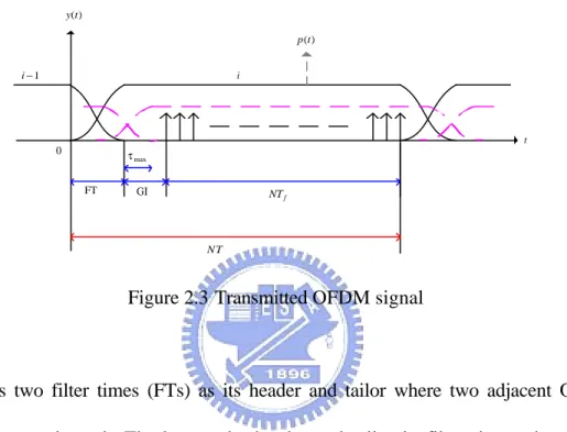
2.3 Transmitted OFDM signal… … … 7
2.4 Transmitter/receiver signal structure… … … .… .11
3.1 One-tap equalizer for conventional OFDM… … … 15
3.2 One block decision feedback equalizer… … … ...16
3.3 MMSE channel estimation… … … .20
3.4 Adaptive equalizer of BE-OFDM… … … ...22
3.5 Signal- flow graph representation of LMS adaptive equalizer… … … 24
3.6 Signal- flow graph representation of RLS adaptive equalizer… … … 26
3.7 LMS channel tracking structure… … … .28
3.8 Signal- flow graph representation of LMS channel tracking… … … ..30
3.9 RLS channel tracking structure… … … ..31
3.10 Signal- flow graph representation of RLS channel tracking… … … .32
4.1 Transmission data block structure… … … ..38
4.2 Performance of SER with Ω=2… … … .41
4.3 Performance of SER with Ω=1.5… … … 42
4.4 Performance of SER with Ω=1… … … ...43
4.5 MSE of equalizer coefficients in time-variant channel by using LMS algorithm.45 4.6 Performance of SER in time-variant channe l by using LMS algorithm… … … … 46
4.7 MSE of equalizer coefficient in time-variant channel by using RLS algorithm… 47 4.8 Performance of SER in time-variant channel by using RLS algorithm… … … … .47
4.10 Profile of MSE by SNR=35dB… … … .51
4.11 Profile of MSE by SNR=10dB… … … .51
4.12 SER on effect of length of training interval… … … .52
4.13 MSE of channel on effect of time variant… … … 53
4.14 SER on effect of time variant… … … ...54
4.15 MSE of channel on different efficiency of bandwidth usage… … … ...55
4.16 SER performances on different efficiency of bandwidth usage… … … ...56
4.17 Learning curves of LMS channel tracking in static channel, SNR=30dB… … ...57
4.18 MSE of LMS channel tracking in static channel… … … ..58
4.19 MSE of LMS channel tracking in time variant channel… … … ...59
4.20 Learning curves of LMS channel tracking in time variant channel, SNR=10dB… … … ...60
4.21 Learning curves of LMS channel tracking in time variant channel, SNR=25dB… … … ...60
Chapter 1
Introduction
Orthogonal frequency-division multiplexing (OFDM) is generally known as an effective technique for high bit rate applications such as digital audio broadcasting (DAB) [1], digital video broadcasting (DVB) [2], and wireless local area networks (WLANs) Such as IEEE 802.11 and HIPERLAN [3], [4].
The basically OFDM system inserts a time-domain guard interval (GI) at the transmitter. It can prevent intersymbol interference (ISI) and can mitigate frequency selectivity of a multipath channel with using a simple one-tap equalizer at receiver end. The GI is the OFDM symbol cyclically extended to avoid interblock interference (IBI) and each truncated block signal is fast Fourier transform (FFT) processed, an operation converting the frequency-selective channel into parallel flat- faded independent subchannels with the length of the GI more than channel delay spread. The intercarrier interference (ICI) can be cancelled using one-tap equalizer.
In all, the GI has advantages of cancellatio n IBI and mitigation of frequency selectivity. In opposition to, the GI has disadvantage of reduced date rate and poor bandwidth efficiency, because, the GI is the excess symbol to an OFDM symbols.
The bandwidth is an important resource in wireless communications. Due to limited bandwidth, increasing bandwidth efficiency is becoming more invaluable in wireless multimedia services. In this thesis, we will focus on enhanc ing bandwidth efficiency in OFDM system. There have been several studies to improve the efficiency of bandwidth usage for the conventional OFDM system. These studies can be divided into several methods. The first method is channel impulse response shorting. To avoid using a long GI, a short time-domain finite impulse response filter is used to shorten the effective channels impulse response, such as Melsa and Younce [5]. The second method is the optimum equalizer based on a minimum mean square error (MMSE) criterion and maximum geometric signal- to noise ratio (GSNR)[6]. The third method studied performance of several equalizers without GI such as Vandendorpe [7], Kim, Kang and Powers [8]. In addition to these studies, there is a further by Sun [9] that we must not ignore, because it can adjust GI length to any desirable bandwidth efficiency.
In this thesis, we focus on this bandwidth efficient OFDM (BE-OFDM) structure [9] and design the channel equalizer and channel estimation. The BE-OFDM system structure will first be introduced. Next, channel equalizer and channel estimation will follow.
For channel equalization, Sun [9] uses one block decision feedback equalizer (DFE). This channel equalizer is a time domain equalizer. It is an effective equalizer to cancel serious ISI. But, the time domain equalizers are usually more complex than the freque ncy domain equalizers, especially the time domain DFE. Besides, Sun [9] adopts oversampling at the receiver end, and the channel equalizer is more complex. In this thesis, we will examine the problems of oversampling and equalizer complexity of BE-OFDM system, and try to reduce comp lexity of one block DFE.
In conventional OFDM, channel estimation is an important issue. If channel estimation can be very accurate, then we only need a simple one-tap equalizer in frequency domain. It can be successful in recovering symbol. In BE-OFDM system, because the time-domain one block equalizer issued, accuracy channel estimation is needed. O ur channel estimation includes training and tracking part. In the training part, we adopt minimum mean square error criteria. In which, we need to rewrite receiver signal with channel fading gain vector and transmitter signal matrix. In the tracking part, we propose the channel tracking structure, rather than an adaptive equalizer. In this structure, the accuracy of estimated equalizer coefficient is better than the adaptive equalizer method, but the complexity of channel-tracking algorithm is higher. Besides, we propose to use the balanced step-size control. It can improve the problem of slow channel tracking.
We use both static and time variant channels [10] to simulate and compare channel equalization and channel estimation. To start with, the channel equalizer tests efficiency of bandwidth usage and system complexity by the static channel. Next, we can see mean square error in the time variant channel. Finally, the performance and efficiency of all systems are compared.
The rest of the thesis is organized as follows. In chapter 2, we will introduce the conventional OFDM system and BE-OFDM system. Efficiency of bandwidth usage will be defined. In chapter 3, the channel equalizer and channe l estimation will be introduced. Besides, we will also introduce LMS and RLS methods for channel tracking. Computer simulations will be given in chapter 4 and the conclusion in chapter 5.
Chapter 2
Bandwidth-Efficient OFDM system
model
In this chapter, we will introduce conventional OFDM and bandwidth efficiency OFDM (BE-OFDM) system. The BE-OFDM system distinguishes itself in capability of free adjustment of the efficiency of bandwidth usage. But, this system will be more complex than conventional OFDM system in the channel equalizer. This problem of the channel equalizer will be discussed in chapter 3. Both systems can operate on time- variant channels and we will define their efficiency of bandwidth usage. Finally, we will compare conventional OFDM system with BE-OFDM system.
In section 2.1, the conventional OFDM system will be introduced and discussed. In section 2.2, we will describe the BE-OFDM system. The efficiency of bandwidth usage will be introduced in section 2.3. In section 2.4, we will compare conventional OFDM and BE-OFDM.
2.1 Conventional OFDM system
consideration is shown in Fig. 2.1 ) (t x ) (t y ) ( ˆ i s s T ) (i F y ) (i y ) (i sn s(i) ) ( ˆ i sn
Figure 2.1 Conventional OFDM system
In transmitter end, several input bits modulate one data symbol sn(i) by M-PSK, and then N data symbols are combined into one block data symbol s(i), and the block data symbol is transferred by the serial-to-parallel converter to the OFDM modulator. After, each block data symbol is modulated by the corresponding subcarrier, the cyclic prefix (CP) is inserted in front. The modulation block signal and the added CP part define one OFDM symbol. Next, these OFDM symbol passes through the parallel- to-serial converter and digital-to-analog converter to turn into a transmitter signal x(t).
The multipath channels will be considered in this system. In general, CP length must be more than channel delay spread [11]. That is to prevent interblock interference (IBI) and to mitigate frequency selectivity of a multipath channe l. Next, the receiver signal y(t) is sum of an additive white noise and the multipath channel output of the transmitter signal.
by corresponding subcarrie r. Next, one-tap equalizer compensates for channel frequency response. Finally, using the demodulation of M-PSK demodulator recurs. We shall have more to say about one-tap equalizer in section 3.1
2.2 Bandwidth-Efficient OFDM system
The Bandwidth-Efficie nt OFDM (BE-OFDM) system and conventional OFDM system have different structures. Their main difference is CP. The former can be free to adjust CP length according to desired bandwidth efficiency. The latter can’t adjust the length of CP, according to desired which is pre-determined by the channel delay spread length. Next, we will discuss the BE-OFDM system [9] structure as shown in Fig. 2.2. ) (t x ) (t y ) ( ˆ i s s T ) ( ˆ i sn ) (i y ) (i s ) (i sn
Figure 2.2 Bandwidth-Efficient OFDM system structure
There are N data symbols in the thi OFDM block sn(i). The transmitted baseband OFDM signal can be expressed as
∑∑
∞ − − × − − − = t inT N n j N 1 2π ( 1)( )where j = −1, a is a DFT constant va lue, T is the data symbol period and NT
is an OFDM symbol period. In Eq.(2.1), p(t) is the OFDM pulse-shaping filter that is usually a time-domain raised cosine function and will be depicted in Appendix A. It is shown by the solid line in Fig. 2.3.
f NT N T max τ FT GI i 1 − i ) (t y t ) (t p 0
Figure 2.3 Transmitted OFDM signal
) (t
p has two filter times (FTs) as its header and tailor where two adjacent OFDM pulses are overlapped. The longer the header and tailor in filter times, the shorter
) (t
p ’s header and tail in frequency domain Except for in the filter time, p(t) is flat in an OFDM period, namely, p(t)=constant for t∈[FT,NT]. It is defined that p(t)=0 if t∉[0,NT]. The frequency spacing between adjacent subchannels is
) /(
1 NTf . If the header and the tail of the pulse-shaping filter in frequency domain are ignored, 1/Tf is close to the total bandwidth of the transmitter signal x(t). The
frequency offset (N−1)/(2NTf ) makes the frequency band of x(t) symmetric to the origin.
∑
= − + = d q q q t x t v t t y 1 ) ( ) ( ) ( ) ( α τ (2.2)where v(t) is an additive white Gaussian noise with power spectrum density N0 /2.
d is the number of paths. αq(t) is the channel fading coefficient of the q th path,
whose magnitude is Rayleigh-distributed and the phase is uniformly distributed. τq is the propagation delay of the q th path. Assume that τ1 =0, τq >0 for q >1
and
{
d}
<NT= τ τ
τmax max 1,K, (2.3) In practical systems, the OFDM period NT is usually designed to be much larger
than the channel delay τmax.
The received continues-time baseband signal is then
∑∑
∞∑
−∞ = − = = − − − − + × − − = i N n d q iNT t N n NT j q q n i t p t iNT e v t s a t y q f 1 0 1 ) )( 2 1 ( 2 ) ( ) ( ) ( ) ( ) ( τ π τ α (2.4)As demonstrated in Fig. 2.3, only OFDM blocks i−1 and i are involved in y(t)
within the i th OFDM period t∈[iNT,(i+1)NT]. Suppose that N samples with s
sampling period T are taken in time interval s [iNT +t0,(i+1)NT] with
s sT N NT t ≤ − ≤ 0
0 . Note that the first sample in the i th OFDM period is taken at
0
t
iNT + . Hence, if t0 >Ts, the received signal in interval [iNT,ιNT +t0] of the th
i OFDM period is discarded. If t0 =0, then the signal in each entire OFDM period is sampled. Assume that the timing is perfect so that only OFDM blocks i−1 and i are involved in N samples. The s k th sample in the i th OFDM period is
(
)
( ) ) ( ) ( ) ( ) ( ) ( ) ( 0 ) ( 2 1 2 0 1 1 0 1 0 0 0 s kT t NT m i N n NT j j s i i m N n d j s q n s k kT t iNT v e kT t NT m i p kT t iNT i s a kT t iNT y i y q s f + + + × − + + − + + = + + = − + + − − − − = − = =∑ ∑
∑
τ π τ α (2.5)The yk(i) can be also equivalent to
( ) ( ) ) ( ) ( ~ ) ( ) ( ) ( ) ( ) ( ) ( 1 0 1 0 , 1 ) ( , ) ( , 0 2 1 2 2 1 2 0 1 0 1 0 1 0 0 i v m i s f e c kT t iNT v m i s ae e kT t mNT p kT t NT i y k m n N n n k d q m n q m q k s n kNT N n NT j t mNT N n NT j q s m N n d q s q k s f q f + − = + + + − × × × − + + × + + =
∑ ∑ ∑
∑∑∑
= − = = − − ′ − + − − = − = = ι τ ι α π τ π (2.6)where for m=0 and 1, and
) ( ) ( ) ( 0 0 ) ( , q s s q m q k i iNT t kT p mNT t kT c =α + + × + + −τ (2.7) ( q j) f t mNT N n NT j m n q e e τ π + − − − = 0 2 1 2 ) ( , (2.8) ( s) f kNT N n NT j n k ae f − − = 2 1 2 , ~ π (2.9) vk(i)=v(ιNT +t0 +kTs) (2.10) and we take a =1/ NTf /Ts . The collected signal samples in a matrix form can be written as y(i) ≡
[
y0(i) L yN−1(i)]
T , s(i)≡[
s0(i) L sN−1(i)]
T and[
]
T N i v i v i s () ) ( ) ( ≡ 0 L −1 v . Let[
m]
N d j k m (i) = c( )(i) ∈C s× , ) ( C (2.11)[ ]
m d N n j m C e ∈ × = (,) ) ( E (2.12)[ ]
N N n k s C f ∈ × = ~, F (2.13)then combine Eq.(2.11) and Eq.(2.12) to form G(m)(i)=C(m)(i)E(m) ∈CNs×N (2.14) and F G H(m)(i)= (m)(i)o (2.15) where the operation o denotes the Hadamard product. Thus, the vector of collected samples is ( ) (0)() () (1)() ( 1) ( ) i i i i i i H s H s v y = + − + (2.16)
where the v(i)~N(0,σ2I) with N /0 Ts
2 =
σ . Next, we need i.i.d. assumptions of signal and noise as follows.
[
]
[
]
[
n n]
2I 2 * 1 2 1 2 1 2 1 ) ( ) ( (3) 0 ) ( ) ( (2) ) ( ) ( ) ( ) ( (1) σ ι ι ι ι δ ι ι δ ι ι = = − − = E n s E n n s s E b n b a n na bIn some applications, the radio channel can be treated as time- invariant within one OFDM period, i.e.
) ( ) (iNT t0 kTs q iNT q α α + + ≅ (2.17)
Jakes model [12] can be used to model the multipath channel with independent Rayleigh fading [10] in each path.
We can know the receiver signal samples from Eq. (2.16). Next, we need the one block decision feedback equalizer (DFE) to estimate block data symbol. The main propose of the equalizer is to cancel serious intersymbol interference. But, its structure is rather complex. The detailed discussion of this equalizer will be presented in section 3.1. One final point is using demodulation of M-PSK for symbol recovery.
Next, we can explain transmitter/receiver signal structures of conventional OFDM and BE-OFDM by Fig. 2.4 and 2.5
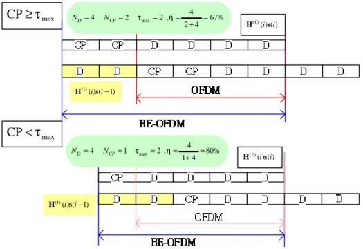
max CP<τ max CP≥τ ) 1 ( ) ( ) 1 ( i si− H ) ( ) ( ) 0 ( i si H % 80 4 1 4 , 2 1 4 max = + = = = = CP τ η D N N ) 1 ( ) ( ) 1 ( i si− H ) ( ) ( ) 0 ( i si H % 67 4 2 4 , 2 2 4 max = + = = = = CP τ η D N N
Figure 2.4 Transmitter/receiver signal structure
In Fig 2.4, when length of CP is longer than channel delay spread, transmitter signal structure is combined by data and CP. In receiver end, conventional OFDM remove CP to make IBI and ICI free. BE-OFDM doesn’t remove CP, so it contains IBI. When length of CP is shorter than channel delay spread, conve ntional OFDM will have serious IBI. Therefore, one-tap equalizer can not detect data signal successfully. But, one block DFE in BE-OFDM can solve this problem due to DFE.
2.3 Efficiency of bandwidth usage
In the framework of many OFDM systems, most stud ies on channel equalization do not discuss the efficiency of bandwidth usage of their systems. However, the efficiency of bandwidth usage has important meaning in wireless communications. If we have high efficiency of bandwidth usage, this implies that we squander not too much the bandwidth resource. Therefore, discussion of efficiency of bandwidth usage is one of the most significant problems in the thesis.
Before we define efficiency of bandwidth usage, we must understand meanings of some parameters in BE-OFDM system, such as T , Tf and N are transmitter
parameters determining transmitted OFDM signal, and N , s T and s t are receiver 0
parameters that determine how to use the received signal. In section 2.2, we have already discussed that the transmitter bandwidth can be approximated as the reciprocal of Tf . The data symbol time is equal to T in BE-OFDM system. Assume that T and N are fixed, then Tf determines not only the bandwidth but also the efficiency of bandwidth usage and the dimensions of the transmitted continues signal. The efficiency of bandwidth usage is defined as
T Tf = = Bandwidth rate symbol Data η (2.18)
For the general OFDM system, we can specify the bandwidth 1/Tf to achieve an arbitrary efficiency of bandwidth usage. However, for an OFDM system to possess some special characteristics, the bandwidth might be determined by other parameters of both transmitter and receiver. To adjust the efficiency of bandwidth usage η, we may consider the following case:
(1) η <1: This implies sufficient freedom is provided for the transmitter (2) η =1: The bandwidth is equal to the Nyquist bandwidth for the transmitter (3) η >1: The system is overloaded in the sense that more symbols
than the signal dimensions are transmitted
The overloaded OFDM system is similar to an overloaded DS-CDMA system that accommodates a larger number of users than the processing gain.
2.4 Comparison of conventional OFDM and BE-OFDM
Convent ional OFDM and BE-OFDM systems have several different points. From Fig 2.1 and 2.2, we can see that conventional OFDM and BE-OFDM systems use one-tap equalizer and one block decision feedback equalizer, respectively. The detail of channel equalizer will be discussed in chapter 3.
In conventional OFDM system, guard interval needs to be long than channel delay spread, and it can be free of interchannel and interblock interference. This imposes a relationship on the transmitter/receiver parameters. Therefore, conventional OFDM system can not arbitrarily adjust efficiency of bandwidth usage. In BE-OFDM system, efficiency of bandwidth usage can be adjusted. So, BE-OFDM system will have the problem of IBI and ICI. But, one-block DFE can improve the problem of IBI and ICI. If conventional OFDM or BE-OFDM systems is free of IBI and ICI, then
) ( ) 1 ( i
H of Eq. (2.16) will be a zero matrix.
Finally, we can summarize comparison of conventional OFDM and BE-OFDM systems by Table 2.1 parameters Conventional OFDM system BE-OFDM system Bandwidth
efficiency Poor Good
Interference IBI and ICI
free IBI and ICI
Channel equalizer One-tap equalizer One block DFE Computational
complexity Low High
Chapter 3
Channel Equalizer and Channel
Estimation
In this chapter, we will introduce channel equalizer and channel estimation in BE-OFDM system. Channel equalizer will use one block decision feedback equalizer. The channel estimation will contain the estimation of training and tracking. Training will use MMSE criteria and tracking will use with adaptive equalizer and adaptive channel tracking. Finally, adaptive channel tracking will be improved by the technique of balanced step-size control.
The channel equalizer of conventional and BE-OFDM systems will be introduced in section 3.1. In section 3.2, the training part will use MMSE criteria for channel estimation. In section 3.3 and 3.4, adaptive equalizer and adaptive channel tracking will be introduced, respectively. In adaptive channel tracking, slow tracking will be improved by method of average step size. Adaptive equalizer and adaptive channel tracking will be compared in section 3.5.
3.1 Channel equalizer
In this section, we will design channel equalizer for conventional OFDM and BE-OFDM systems, respectively. First, conventional OFDM system uses usually one-tap equalizer. Second, BE-OFDM system uses one block equalizer
3.1.1 One-tap equalizer for conventional OFDM
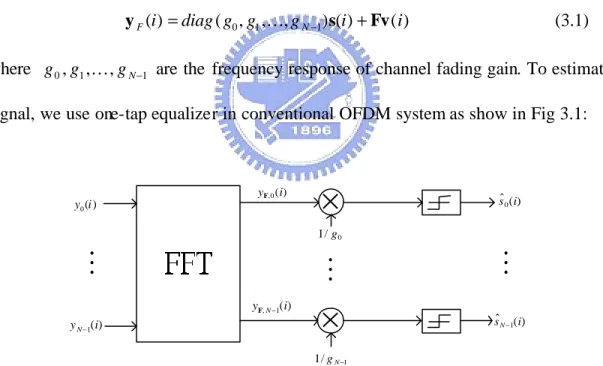
The conventional OFDM system is given in Fig. 2.1. In general, one-tap equalizer is used in conventional OFDM system that compensates channel frequency response. After removing CP and passing through FFT matrix, we can write the received signal in frequency domain by
) ( ) ( ) , , , ( ) (i diag g0 g1 gN 1 i i F s Fv y = K − + (3.1)
where g0,g1,K,gN−1 are the frequency response of channel fading gain. To estimate signal, we use one-tap equalizer in conventional OFDM system as show in Fig 3.1:
×
×
0 / 1 g 1 / 1 gN− ) ( 0i y ) ( 1i yN− ) ( ˆ 0i s ) ( ˆ 1i sN−M
) ( 0 , i yF ) ( 1 , i yFN−M
M
Figure 3.1 One-tap equalizer for conventional OFDM
From Eq. (3.1), we can produce the reciprocal of g0,g1,K,gN−1 and we get the
estimated signal by ˆ( ) decision of
{
( , , , ) 1 ()}
1 1 0 g g i g diag i N yF s = K − − (3.2)problem, and its channel equalizer will use one-tap equalizer.
3.1.2 One Block equalizer for BE-OFDM system
Block equalizer [13], [14] are considered in many communication systems. The method of block equalizer is rarely seen in OFDM system or multicarrier communications system. But, BE-OFDM system that cancels serious ISI needs to use block equalizer. Besides, from Eq. (2.16) can see that the energy of received signal is concentrated on (0)( )
i
H . Because of an OFDM period is designed to be longer than the channel delay spread, this suggests the use of a DFE structure in channel equalization for BE-OFDM system.
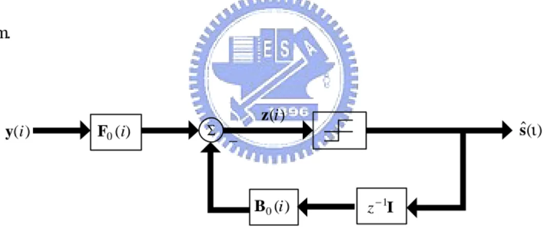
Fig. 3.2 is one block decision feedback equalizer structure for BE-OFDM system. ) (i y ∑ − ) (i z ) ( ˆι s ) ( 0 i F ) ( 0 i B z−1I
Figure 3.2 One block decision feedback equalizer
The signal before decision is given by
z(i)=F0(i)y(i+1)−B1(i)ˆs(i−1) (3.3) where sˆ(i−1) is the pervious estimate of s(i−1). F0(i)∈CN×Ns and B1(i)∈CN×N
are matrices representing the forward and the backward filters, respectively. One block DFE will use MMSE criteria as
[
2]
) ( ), ( () ( ) min DFE E i i i B i F mse = z −s (3.4)Next, substituting Eq. (3.3) into Eq. (3.4)
[
2]
1 0 ) ( ), ( ) ( ) 1 ( ˆ ) ( ) 1 ( ) ( min DFE 1 0 i i i i i E i B i F mse = F y + −B s − −s (3.5)By principle of orthogona lity, the gradients of forward and backward filters are written by
(
)
[
y F y −B s − −s]
=0 − = ∇ * 1 0 0 ) ( ) 1 ( ˆ ) ( ) ( ) ( ) ( 2 ) ( DFE i i i i i i E i F mse (3.6)(
)
[
s F y B s s]
0 B =− − − − − = ∇ * 1 0 1 ) ( ) 1 ( ˆ ) ( ) ( ) ( ) 1 ( ˆ 2 ) ( DFE i i i i i i E i mse (3.7)Assume that demodulation of previous block is perfect. Since
[
s( i)s*( j)]
(i j)IE ι− ι− =δ − (3.8)
[
s ( −i)v ( − j)]
=0E n ι k ι (3.9) for all n,k,i, j. Then, we find the coefficients of backward filter as
) ( ) ( )] 1 ( ˆ ) ( [ ) ( ) ( ) 1 ( 0 * 0 1 i i i i E i i H F s y F B = − = (3.10) where
[
]
[
(
)
]
) ( ) 1 ( ) ( ) 1 ( ) ( ) ( ) ( ) 1 ( ˆ ) ( ) 1 ( * ) 1 ( ) 0 ( * i i i i i i i E i i E H s v s H s H s y = − + − + = − (3.11)Next, the coefficients of forward filter are written as.
[
] [
(
]
)
(
(0) (0) 2)
1 ) 0 ( 1 ) 1 ( ) 1 ( * * 0 ) ( ) ( ) ( ) ( ) ( ) ( ) ( ) ( ) ( ) ( * * − − + = − = I H H H H H y y s y F n i i i i i i i E i i E i σ (3.12) where[
]
[
(
)
]
) ( ) ( ) ( ) 1 ( ) ( ) ( ) ( ) ( ˆ ) ( ) 0 ( * ) 1 ( ) 0 ( * i i i i i i i E i i E H s v s H s H s y = + − + = (3.13)[
]
[
(
)
()
]
I H H H H v s H s H y y 2 * ) 1 ( ) 1 ( * ) 0 ( ) 0 ( * ) 1 ( ) 0 ( * ) ( ) ( ) ( ) ( ) ( ) 1 ( ) ( ) ( ) ( ) ( ) ( n i i i i i i i i E i i E σ ι + + = ⋅ + − + = (3.14)From Eq. (3.10) and Eq. (3.12), we can get the coefficients of backward and forward filter, respectively.
3.1.3 Reduced One Block DFE complexity
In section 3.1.2, we knew structure of one block DFE as Fig. 3.2. The coefficients of backward filter in Eq. (3.10) and coefficients of the forward filter in Eq. (3.11) are very complex to find. In the forward part, it needs an inverse matrix with the N by s N . Where s N is the number of samples of one OFDM symbol at s
receiver end. In other words, the size of N will determine the complexity of the s
forward filter.
From section 2.2, received continuous time signal is sampled in Eq. (2.6). But, we must have (1) Ns ≥ N to obtain sufficient dimensions of sampled signal for symbol demodulation and (2) Ts ≤Tf so that Nyquist sampling rate is satisfied.
Added to this, N needs to satisfy s
= = s f s s T T N ceil T T N ceil N η 1 (3.15)
where N is combined with the number of subcarriers, efficiency of bandwidth s
usage and oversampling factor Ω, which is defined as
s f T T = Ω (3.16)
In Eq. (3.15), only oversampling factor can be adjusted. Because, N and η are predetermined by system.
From what has been said above, we can obtain a small conclusion, that is, complexity of the forward filter is relative to oversampling factor. That is to say, the size of oversampling factor will influence complexity of one block DFE. The problem of adjusting Ω will be discussed further in chapter 4.
3.2 Training part of channel estimation for BE-OFDM
system
In BE-OFDM system, channel estimation will be divided into parts of training and tracking. In this section, we will the discuss part of training in channel estimation. It is based on the minimum mean square error (MMSE) criteria. Before turning to the part, we must describe signal model.
3.2.1 Signal model in training
To use the MMSE criteria, we must rewrite receiver signal model of Eq. (2.16) as ) ( ) ( ) ( ) ( ) ( ) (i S(0) i a i S(1) i a i v i y = + + (3.17)
where S(0)(i a) (i) and S(1)(i a) (i) are transformed from by (0)( ) ()
i i s H and ) 1 ( ) ( ) 1 ( − i i s
H , respectively. Let us now look at their transformation process in detail. First, from Eq. (2.15) know that H(m)(i)s(i) can written as
() () ~ ( ) m 0,1 1 0 , ) ( , 1 ) ( , ) ( = =
∑ ∑
− = = i s f e c i i n N n n k m n q d q m q k m s H (3.18)(
)
[ ]
(
)
[
]
{
}
0.1 m ) ( ) ( ) ( ~ ) ( ] [ ) ( ~ 1 ) ( ) ( ) ( ) ( ) ( ) ( , 1 1 0 ) ( , , , 1 ) ( , ) ( = = = =∑ ∑
= − = i i i i i e f i s v i i m T m T m k j d q N n m j n n k k n m q k m a S a E F 1 s v s H o o α (3.19) where 11,k =1, Ns k × ∈ = 1 , 1 ] C 1 [1 , a(i) is the channel fading gain in one OFDM symbol , and S(m)(i) is given by
[ ]
(
)
[
() ~]
m 0,1 ] [ ) ( ( ) ( ) ) (m = m T mT = i i v s 1 FE S o o (3.20)which
( )
⋅ Tdenote the transpose and S(m)(i)∈CNs×d .3.2.2 Training: MMSE channel estimation
To obtain channel information, we will use the training symbol to estimate channel impulse response. At the same time, we can use MMSE criteria. First, let us define ) ( ) ( ) (i S(0) i S(1) i S = + (3.21) ) ( ) (i a i h = (3.22) Then, Eq. (3.17) can be written as t
) ( ) ( ) ( ) (i S i h i v i y = + (3.23) Next, we will show how to estimate channel impulse response in Fig. 3.3
)
(i
y
ST
S
(i
)
)
(i
s
)
(
ˆ i
h
The MMSE criteria is given by
[
]
− = − = 2 )) ( ˆ 2 ) ( ˆ ) ( ) ( ˆ ) ( min ) ( ) ( ˆ min i i i E i i E mse y h S y y H h h ι ι (3.24)where estimation of receiver signal is given by
yˆ(i)=S(i)hˆ(i) (3.25) By principle of orthogonality, the gradient vector of Hmse with hˆ i( ) is set to be zero:
(
)
0 y h S H h h = − ∇ = ∇ ) ( ) ( ˆ ) ( 2 ) ( ) (i mse i E i i i (3.26)We can obtain channel estimate by
[
]
(
)
[
]
(
( ) ( ))
() ( ) ) ( ) ( ) ( ) ( E ) ( ˆ * 1 * * 1 * i i i i i i E i i i y S S S y S S S h − − = = (3.27)where receiver signal y(i) and transmitted signal S(i) are known to us, so S(i)’s autocorrelation, S(i) and y(i)’s crosscorrelation are given by
[
() ()]
( ) ( ) ES* i S i =S* i S i (3.28)[
*() ( )]
*() () i i i i ES y =S y (3.29) AS mentioned above, we can use the training symbol S(i) to obtain the MMSE channel of estimate.3.3 Adaptive Equalizer
In this section, we will introduce the adaptive equalizer to the BE-OFDM system. Why introduce the adaptive equalizer? Because, we wish that adaptive equalizer can complete the tracking of equalizer coefficients in successive two OFDM symbols.
Here, we will use least- mean-square (LMS) and recursive-least-square (RLS) [15] in adaptive equalizer [16], respectively.
3.3.1 LMS adaptive equalizer
In this section, the LMS algorithm is used to update equalizer coefficients in adaptive equalizer. First, the adaptive one block DFE is given in Fig. 3.4.
) (i y − ) (i z ) ( ˆ i s ∑ ∑ − ) ( 0 i F ) ( 0 i B z−1I
Figure 3.4 Adaptive equalizer of BE-OFDM
The mean square error (cost function) between equalizer output and estimated signal can be defined in the i thOFDM symbol period as
) ( ) ( ) ( * , i i i JAEQLMS =e e (3.30) where the error of estimation is given by
) ( ˆ ) ( ) ( ) ( ) ( 1 0 i i i e i e i N s z e = − = − M (3.31)
The estimation error is an N by 1 vector. We can the rewrite output of one block DFE z(i) in Eq. (3.3) as
) ( ) ( ) (i W i u i z = (3.32) where the coefficients of one block DFE can be written by
[
( ) ( )]
)(i F0 i B1 i
W = − (3.33) The size of this matrix is N by (Ns +N), and the input vector of DFE is given by
− = ) 1 ( ˆ ) ( ) ( i i i s y u (3.34)
The size of this vector is (Ns +N)by 1. To calculate the estimated of gradient vector )
( ˆ
, i
JAEQLMS
∇ , we can extend the cost function by substitution of Eq. (3.31) and (3.32) to Eq. (3.30),
(
( ) ( ) ˆ()) (
( ) () ˆ())
) ( * , i i i i i i i JAEQLMS = W u −s W u −s (3.35) Correspondingly, estimation of gradient vector is given by) ( ) ( ) ( 2 ) ( ) ( ˆ 2 ) ( ˆ * * i i i i i i J =− s u + u u W ∇ (3.36)
We get a recursive relation for updating of coefficients of one block DFE as
) ( ) ( ) ( ) ( ˆ 2 1 ) ( ) 1 ( * , i i i i J i i AEQLMS u e W W W µ + = ∇ − = + (3.37)
From this equation, we can know the update equation of forward and backward filter coefficients are given by
) ( ) ( ) ( ) 1 ( 0 * 0 i F i e i y i F + = +µ (3.38) ) 1 ( ˆ ) ( ) ( ) 1 ( * 1 1 i+ =B i − e i s i− B µ (3.39)
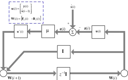
As mentioned above, we can draw a signal- flow graph representation of the LMS algorithm in form of a feedback model as Fig. 3.5.
∑ µ I ) 1 (i+ W W(i) ) (i e z(i) ) ( ˆ i s − + I 1 − z − = ) 1 ( ˆ ) ( ) ( i i i s y u [ () ()] ) (i F0i B1i W = − ) (i u ) ( *i u
Figure 3.5 Signal- flow graph representation of LMS adaptive equalizer
In this figure, signal- flow graph clearly illustrates recursive formula of LMS algorithm in adaptive one block DFE. This LMS algorithm has several special problems. Note that update coefficients of equalizer is not vector. In opposition, it updates one block matrix coefficients. In addition to this, the update equation can be considered as several parallel standard LMS algorithms.
3.3.2 RLS adaptive equalizer
In this section, we will use the recursive least square (RLS) algorithm as our adaptive equalizer. Its structure is show in Fig. 3.4. We express the cost function to be minimized as ) ( ) ( ) ( * 1 , i i i J i k k i RLS AEQ
∑
e e = − = ω (3.40) where ω is a forgetting factor and error of estimation e(i) is given in Eq.(3.31). Substituting e(i) into Eq. (3.40), we get(
() ( ) ˆ( )) (
() () ˆ( ))
) ( * 0 , i i i i i i i J i k k i RLS AEQ =∑
W u −s W u −s = − ω (3.41)value equal to zeros 0 W = ∂ ∂ ) ( ) ( , i i JAEQRLS (3.42)
After some rearrangement, we get the directly adaptive one block DFE as
[
]
) ( ) ( ) ( ) ( ) ( 1 1 0 i i i i i − = − = R D B F W (3.43) where ) ( ) ( ˆ 1) -( ) 1 ( ) ( ) ( ) ( ˆ ) ( * 0 * 0 * i i i k k k k i i k k i i k k i u s D s s y s D + = − =∑
∑
= − = − ω ω ω (3.44) and ) ( ) ( ) 1 ( ) 1 ( ) 1 ( ˆ ) ( ) 1 ( ) 1 ( ) ( ) ( ) ( ) ( * 0 * 0 * 0 * 0 * i i i k k k k k k k k i i k k i i k k i i k k i i k k i u u R s s y s s y y y R + − = − − − − =∑
∑
∑
∑
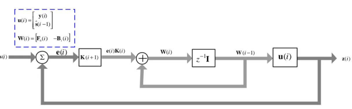
= − = − = − = − ω ω ω ω ω (3.45) Denote R−1(i) as P(i), we get )) ( ) ( )( 1 ( 1 ) (i P i I u i K i P = − − ω (3.45) where ) ( ) ( ) 1 ( 1 ) ( ) ( ) 1 ( ) ( 1 ) ( * * 1 * i i i i i i i i P u P u u P u K = − + − = − ω ω (3.46)Then, substitute Eq. (3.44), (3.45) and Eq. (3.46) into Eq. (3.43), we can obtain the equalizer coefficient update equation as
) ( ) ( ) 1 ( ))} ( ) ( )( 1 ( 1 )}{ ( ) ( ) 1 ( { ) ( * i i i i i i i i i i K e W K u I P u s D W + − = − − + − = ω ω (3.47)
Next, we can draw the signal- flow graph representations of the RLS adaptive equalizer in Fig. 3.6. ) (i s e(i) ) ( ) (i Ki e W(i) ) (i z ∑ −1I W(i−1) z u(i) ) 1 (i+ K − = ) 1 ( ˆ ) ( ) ( i i i s y u [ () ()] ) (i F0i B1i W = −
Figure 3.6 Signal- flow graph representation of RLS adaptive equalizer
This figure clearly illustrates recursive formula of the RLS algorithm in adaptive one block DFE. Its algorithm and LMS are similar, that is, several standard RLS’s make a big RLS algorithm, and it is to update one block matrix coefficients, too.
3.3.3 Summary of adaptive equalizers
In this subsection, we will summarize adaptive equalizers in BE-OFDM system, this contains LMS and RLS algorithm of adaptive equalizer. Table 3.1 and 3.2 summarizes LMS and adaptive equalizers, respectively.
Table 3.1 Computation procedures of LMS adaptive equalizer
(
)
{
}
(
)
[
]
) ( ) ( ) ( ) 1 ( ) ( ˆ ) ( ) ( t coefficien equalizer king trac ) ( ) ( ) ( ) ( ˆ ) ( ) ( ) ( ˆ ) ( ˆ ) ( ˆ ) ( ) ( ˆ ), ( ˆ ) ( ) ( ) ( ) ( ) ( ˆ part ning trai ) 1 ( ˆ ) ( ) ( 1 or input vect ) 0 ( ˆ value initial * 1 0 ) 1 ( 0 1 1 2 ) 0 ( ) 0 ( ) 0 ( 0 ) 1 ( ) 0 ( * 1 * * i i i i i i i i i i i i i i i i i i i i i i i i i i i i n u e W W s z e B F W H F B I H H H F H H y S S S h s y u 0 s H T µ σ + = + − = − = = + = → = − = > = − −Table 3.2 Computation procedures of RLS adaptive equalizer
(
)
{
}
(
)
[
]
) ( ) ( ) 1 ( ) ( )) ( ) ( )( 1 ( 1 ) ( ) 1 ( 1 ) ( ) ( ) 1 ( ) ( 1 ) ( ) ( ˆ ) ( ) ( t coefficien equalizer king trac ) ( ) ( ) ( ) ( ˆ ) ( ) ( ) ( ˆ ) ( ˆ ) ( ˆ ) ( ) ( ˆ ), ( ˆ ) ( ) ( ) ( ) ( ) ( ˆ part ning trai ) 1 ( ˆ ) ( ) ( 1 or input vect ) 0 ( ) 0 ( ˆ value initial * 1 * 1 0 ) 1 ( 0 1 1 2 ) 0 ( ) 0 ( ) 0 ( 0 ) 1 ( ) 0 ( * 1 * 1 * i i i i i i i i i i i i i i i i i i i i i i i i i i i i i i i i i i i i i i n K e W W K u I P P P u u P u K s z e B F W H F B I H H H F H H y S S S h s y u I P 0 s H T + − = − − = − − + = − = − = = + = → = − = > = = − − − − ω ω ω σ δ3.4 Channel tracking in BE-OFDM system
In section 3.3, we have introduced the adaptive equalizer in BE-OFDM system. The main disadvantage of adaptive equalizer is that it is unable to follow accurately
the variation of equalizer coefficients. We shall have more to explain about this disadvantage in adaptive equalizer latter on chapter 4. Here, to replace adaptive equalizer, we propose the structure of channel estimation. Both LMS and RLS algorithms will be used channel tracking.
3.4.1 LMS channel tracking
Now, we shall discuss LMS channel tracking, shown in Fig 3.7.
) (i y − ∑ z(i) sˆ i() ∑ H T ) (l e ) ( ˆl y s N i⋅ = l ) ( ˆ* i S ) ( * l u s ( )* s T ( )* u T − ) ( ˆ i h ) ( 0 i F I 1 − z ) ( 0 i B ) (l y ) ( ˆ l temp h
Figure 3.7 LMS channel tracking structure
First of all, we shall explain several blocks in Fig. 3.7
(1) T : The signal of estimation S sˆ i() is transformed to the convention signal
matrix of estimation Sˆ i() by this block function. Conventional signal
matrix of estimation combines Sˆ(0)(i) with S(1)(i) as Eq. (3.20)
substituted into Eq. (3.21)
k N i− ⋅ s + =( 1) l (3.48) for k =1,2,K,Ns.
(3) T : The channel fading gain of estimation H hˆ i() can be transformed the main matrices of conventional channel H(0)(i) and interblock interference conventional channel H(1)(i) in Eq. (2.15)
After discussing functions of blocks in Fig. 3.7, we will introduce LMS algorithm channel tracking algorithm. To begin with, we will define the mean square error (cost function) of both receiver sample and estimation receiver sample as
) ( ) ( ) ( * , l e le l JCTLMS = (3.49) where error of estimation is defined as
e(l)= y(l)−yˆ(l) (3.50)
) (L
y is an element of the receiver signal vector y(i) and ) ( ˆ ) ( ) ( ˆl * l l temp y =su h (3.51)
where hˆtemp(l) is the temporary channel fading gain. Next, we need Eq. (3.50) and Eq. (3.51) substituted into the cost function Eq. (3.49) as
(
( ) ( )ˆ ( )) (
( ) ( )ˆ ( ))
) ( * * * ,LMS l l l temp l l l temp l CT y y J = −su h −su h (3.52)Then, the gradient vector is
) ( ) ( 2 ) ( ˆ ) ( ) ( 2 ) ( ) ( 2 ) ( * , l l l l l l l e L y JCTLMS temp u u u u s h s s s − = + − = ∇ (3.53)
and the update equation of temporary channel fading gain is
) ( ) ( ) ( ˆ ) ( 2 1 ) ( ˆ ) 1 ( ˆ , l l l l l l e J u temp LMS CT temp temp s h h h µ µ + = ∇ − = + (3.54) ) ( ˆ l temp
signal- flow graph will be showed in Fig. 3.8. ) 1 ( ˆ l+ temp h hˆtemp(l) ) (l e ) (l y ) ( ˆl y − + µ I + I 1 − z ) (l u s *(l) u s
Figure 3.8 Signal- flow graph representation of LMS channel tracking.
When the sample index equals N in each OFDM symbol period, we get channel s
fading gain as s s temp i N N i)= ˆ ( ) =( −1)⋅ + ( ˆ h l l h (3.55)
Then, channel fading is plugged to the block of T to get H Hˆ(0)(i) and Hˆ(1)(i). Finally, using the channel matrix updates next forward Eq. (3.12) and backward Eq. (3.10) filter coefficients in one block DFE.
3.4.2 RLS channel tracking
Next, we will discuss RLS algorithm for channel tracking. In general, convergence rate of RLS algorithm is faster than LMS algorithm. So we try this algorithm for channel tracking. We shall discuss RLS channel tracking, showed in Fig 3.9.
) (i y − ∑ z(i) sˆ i() ∑ H T ) (l e ) ( ˆl y s N i⋅ = l ) ( ˆ* i S ) ( * l u s ( )* s T ( )* u T − ) ( 0 i F ) ( 0i B −1I z ) ( ˆ i h ) ( ˆ l temp h
Figure 3.9 RLS channel tracking structure
Fig 3.9 and Fig 3.7 are very similar, their difference is the adaptive algorithm, other parts are the same. Here, we use the RLS algorithm. Next, the cost function is
) ( ) ( ) ( * 0 , l e l e l J L k k L RLS CT
∑
= − = ω (3.56) and we can get temporary channel fading gain of estimation ashˆtemp(l)=R−1(l)D(l) (3.57) where ) ( ) ( ) 1 ( ) ( ) ( ) ( 1 l l l l l l d k d k k k u D s D =
∑
u = − + = − ω ω (3.58) ) ( ) ( ) 1 ( ) ( ) ( ) ( * 1 * l l l l l l l l u u R s s s s R k k k k = − + =∑
= − ω ω (3.59)Then, we set P(l) equal to R−1(l). We get
(
1 ( ) ( ))
( 1) 1 ) ( ) ( * 1 − − = = − l l l l l P s K R P u ω (3.60)where ) ( ) ( ) ( ) 1 ( 1 ) ( ) 1 ( ) ( 1 ) ( 1 1 * l l l l l l u u u u s P s P s P s K i = − + − = − ι ω ω (3.61)
Then, we get the temporary channel fading gain of estimation as
(
)
(
)
) ( ) ( ) 1 ( ˆ ) ( ) ( ) 1 ( ) 1 ( ) ( ) ( 1 1 ) ( ˆ 1 * 1 l l l l l l l l l l e d temp temp K h s D P s K h u u + − = + − − − = ω ω (3.62)The signal- flow graph of temporary channel fading gain htemp(l) can be drawn in Fig. 3.10 ) (l y e(l) e(l K) (l) ( 1) ˆ l− temp h ) ( ˆl y ) ( ˆ l temp h − − + z−1I *( ) l u s ) (l K
Figure 3.10 Signal- flow graph representation of RLS channel tracking
From Eq. (3.62), we get temporary channel fading gain in one OFDM period. Then,
) ( ˆ i
h can be replaced by hˆtemp(l) in Eq. (3.55).
3.4.3 Summary of structure of channel tracking
In this subsection, we will summarize structure of channel tracking in BE-OFDM system, in Table 3.3 and 3.4.
Table 3.3 Computation procedures of LMS channel tracking
(
)
N N i i e y y e i i i i i s temp u temp temp u + ⋅ − = = + = + − = = > = − ) 1 ( ) ( ˆ ) ( ˆ )) ( ) ( ) ( ˆ ) 1 ( ˆ ) ( ˆ ) ( ) ( t coefficien equalizer king trac ) ( ) ( ) ( ) ( ) ( ˆ part ning trai ) ( ), y( 1 or input vect ) 0 ( ˆ value initial * 1 * * l l l l l l l l l l l h h s h h y S S S h s 0 s µ ιTable 3.4 Computation procedures of RLS channel tracking
(
)
(
)
N N i i e y y e i i i i i s temp temp u + ⋅ − = = + − = − − = − − + = − = = > = − − ) 1 ( ) ( ˆ ) ( ˆ ) ( ) ( ) 1 ( ˆ ) ( ˆ ) 1 ( ) ( ) ( 1 1 ) ( ) ( ) 1 ( 1 ) ( ) 1 ( ) ( 1 ) ( ) ( ˆ ) ( ) ( t coefficien equalizer king trac ) ( ) ( ) ( ) ( ) ( ˆ part ning trai ) ( ), y( 1 or input vect ) 0 ( ˆ value initial * 1 * * 1 * * l l l l l l l l l l l l l l l l l l l h h K h h P s K P s P s P s K y S S S h s 0 s u u u u ω ι ι ω ω ι3.4.4 Improved LMS channel tracking with balanced step-size
control
In this section, we discuss the channel tracking problem. In subsection 3.4.1, we have discussed LMS channel tracking in BE-OFDM system. The LMS algorithm has a serious problem in time-variant channel, that is, the channel fading gain of
estimation is not to follow the true channel fading.
In Zhou and Holte [17], their experiment shows clearly that LMS algorithm is not to follow the variation of true channel in fast variant of channel. In slow variation of channel, this algorithm can follow true channel. Similarly in Shimamura and Cowan [18], the ir work is not able to keep track with the true channel, too. For example, instantaneous channel mean square error will have ripples in time variant channel. This implies when channel has big variation in short time, the accuracy of channel estimation will be influenced.
In this thesis, we also have similar problem in time variant channel. For LMS channel tracking, this problem will affect channel tracking. Before we discuss that time variant channel determines the choice of step-size, we must first understand the problem of step-size for a static channel. In general, the size of step-size in static channel will determine the convergence rate and minimum mean square error Jmin. For a larger step-size, its convergence rate will be faster and its Jmin is increased.
For time variant channel, the step-size may affect tracking rate. From Eq. (3.54), we can know that length of channel of estimation channel in successive symbols as
) ( ) ( ) ( ˆ ) 1 ( ˆ l l l e l u temp temp h s h + − = µ (3.63)
If elements of su(l e) (l) vector are fixed value, then step-size will determine variation
of estimation channel. Because, we can not know degree of change of true channel at received end, we can not obtain optimum step-size in each sample. So, the step-size can only try different values. If we choice a big step-size, then channel of estimation increases or decreases too much, and the mean square error of channel will become poor. If we choice a small step-size, then channel of estimation will be not to keep up with the true channel. To balance variation of channel, we propose the balanced
![Table 3.1 Computation procedures of LMS adaptive equalizer ( ) { } ( ) [ ] )()()()1( )ˆ()()( t coefficienequalizer king trac)()()( )ˆ()()( )ˆ()ˆ()ˆ()(](https://thumb-ap.123doks.com/thumbv2/9libinfo/8762523.208514/38.894.145.769.129.440/table-computation-procedures-lms-adaptive-equalizer-coefficienequalizer-king.webp)
