運用功率延遲輪廓近似之線性最小均方差通道估計於LTE下行時變通道傳輸

(1)

國立交通大學

電子工程學系電子研究所碩士班

碩士論文

運用功率延遲輪廓近似之線性最小均方差通道估

計於 LTE 下行時變通道傳輸

LMMSE Channel Estimation with Power-Delay

Profile Approximation for LTE Downlink

Transmission over Time-Variant Channels

研究生：楊葆崧

指導教授：林大衛教授

(2)

(3)

運用功率延遲輪廓近似之線性最小均方差通道估

計於 LTE 下行時變通道傳輸

LMMSE Channel Estimation with Power-Delay

Profile Approximation for LTE Downlink

Transmission over Time-Variant Channels

研究生：楊葆崧 Student: Bao-Song Yang

指導教授：林大衛 Advisor: Dr. David W. Lin

國立交通大學

電子工程學系電子研究所碩士班

碩士論文

A Thesis

Submitted to Department of Electronics Engineering & Institute of Electronics College of Electrical and Computer Engineering

National Chiao Tung University in Partial Fulfillment of the Requirements

for the Degree of Master of Science in

Electronics Engineering August 2013

Hsinchu, Taiwan, Republic of China

(4)

(5)

i

運用功率延遲輪廓近似之線性最小均方差通道估

計於 LTE 下行時變通道傳輸

研究生：楊葆崧指導教授：林大衛博士

國立交通大學

電子工程學系電子研究所碩士班

摘要

正交分頻多重進接(OFDMA)技術近年來在行動環境中廣受注目，而且已經應用在許多數位通訊應用中。採用 OFDMA 一個最主要的原因是其抗頻率選擇性衰變的能力。在此篇論文中，我們聚焦於 LTE 與 LTE-A OFDMA 下行通道估測部分。本篇論文最主要採用的通道估測方法為線性最小均方差(LMMSE)通道估測法。在使用 LMMSE 通道估測法於多載波傳輸系統中，我們需要知道通道相關性函數。這在參考訊號(RS)較少的傳輸系統中帶來了問題。為了解決這個問題，我們將通道的功率延遲輪廓做近似，使其可以完全被兩個通道延遲參數所定義，這兩個參數為初始延遲參數以及方均根延遲擴展參數。除此之外，我們發展了一個技術來估測這些參數。為了增進估測參數的準確度，我們引入了虛參考響應生成的概念來達成我們的目標。接著我們可以找到功率延輪廓遲近似所相對應的自相關矩陣。最後藉由這個自相關矩陣，使用 LMMSE 通道估測法來估計次載波上的資訊。我們藉由加成性白高斯雜訊通道來驗證我們的模擬程式以及通道估測方法，接著在幾個多路徑通道做模擬。

(6)

ii

在本篇論文中，我們首先簡介 LTE 與 LTE-A 下行的標準機制。接著，我們依造兩種標準機制分別各傳輸情形下介紹所用的通道估測方法並探討其估測效能。

(7)

iii

LMMSE Channel Estimation with Power-Delay

Profile Approximation for LTE Downlink

Transmission over Time-Variant Channels

Student: Bao-Song Yang Advisor: Dr. David W. Lin

Department of Electronics Engineering

Institute of Electronics

National Chiao Tung University

Abstract

Orthogonal frequency division multiple access (OFDMA) technique has drawn much interest recently in the mobile transmission environment and been successfully applied to a wide variety of digital communications applications over the past several years. One of the main reason to use OFDMA is its robustness against frequency selective fading. We focus on the OFDMA downlink (DL) channel estimation based on LTE and LTE-A.

The main channel estimation method is linear-minimum-mean-square-error (LMMSE) channel estimation in this thesis. In LMMSE channel estimation for multicarrier systems, one needs to know the channel correlation function. This brings up a problem for systems with a small number of reference signals (RSs). To solve this problem, we approximate the channel power-delay profile (PDP) that can completely be described in two channel delay parameters, i.e., the initial delay and the root-mean-square (RMS) delay. In addition, we develop a technique to estimate these delay parameters. For improving the accuracy of the estimated channel delay

(8)

iv

parameters, we employ an idea, producing pseudo RR, to meet our purpose. Then we find the autocorrelation function associated with the approximate PDP. Finally base on this autocorrelation function, do LMMSE filtering to estimate the data subcarrier response. We verify our simulation program and channel estimation methods on AWGN channel and then do the simulation on several multipath channels.

In this thesis, we first introduce the standard of the LTE and LTE-A DL. Then we describe the channel estimation methods we use and discuss the performance in each transmission condition for LTE and LTE-A.

(9)

v

誌謝

於 2013 八月末，這本論文終於要完成了，在這一路上我受到了許多人的幫助。其中最感謝的，莫過於指導教授林大衛老師，在這兩年多的相處中，老師總是一路耐心的引領著我們，對於我們遇到的問題，總是能夠給予我們適切的方向。平時對於我們也是相當的關心，答應我們的承諾，也總是盡心盡力的去完成，特別是在論文來回修改的時期，平常總是中氣十足的老師，為了趕著將修改好的論文交給我們，竟然難得出現了黑眼圈！對於老師的感激之情，學生葆崧難以用筆墨來形容。另外，在這裡也要好好感謝 CommLab 的各位夥伴。林 Group 的各位兄弟：(怪盜基)男鑫、夏銘和信宏，真的很感謝一路上的互相扶持，不論是在修課、做研究以及找工作，我們都毫無保留，認真的給予彼此建議，讓我們都能夠順利的成長，很慶信自己能夠跟你們做夥伴。還有杭 Group、簡 Group 以及桑 Group，一路上有你們的陪伴，不論在研究或者休閒上都讓我常常擁有不同的感受，在這邊小弟祝各位夥伴們皆能早日結交男/女朋友。而已經離開學校的學長們，感謝你們在我遇到各種問題時所給的種種建議，沒有你們的經驗分享，對於研究以及找工作都還不太熟悉的我可能都還要摸索好一陣子，謝謝你們對我的照顧。最後要感謝我的家人、朋友以及陪伴著我八年的宜涵；在研究的路上，在我遇到各種挫折而心情苦悶的時候，心情及口氣有時會不太和善，然而你們總是能夠給予我鼓勵以及陪伴，讓我的內心總是能夠充滿著正面的能量，這邊我真的是由衷地感謝各位的包容以及陪伴。楊葆崧民國一○二年八月於新竹

(10)

List of Figures

2.1 Traditional FDM system versus OFDM system. . . 6

2.2 A baseband equivalent illustration of modulation in an OFDM system. . . . 7

2.3 A baseband equivalent illustration of demodulation in an OFDM system. . . 8

2.4 OFDMA versus OFDM. . . 9

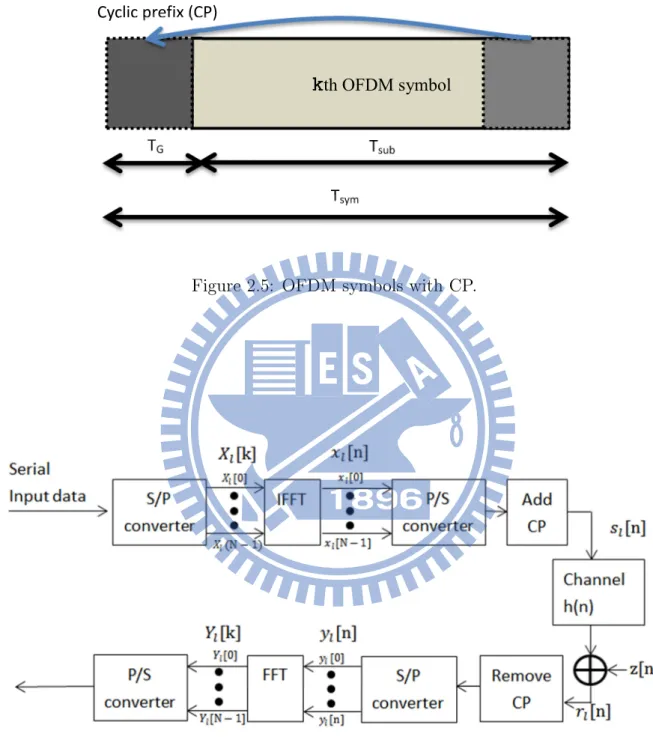
2.5 OFDM symbols with CP. . . 10

2.6 OFDM baseband transmission system structure. . . 10

2.7 Frame structure type 1 [7, Figure 8.2]. . . 12

2.8 Slot structure for normal and extended CP [7, Fig. 8.3]. . . 14

2.9 Overview of physical channel processing [6]. . . 15

2.10 PN sequences generation in the LTE-system [7, Fig. 9.2]. . . 17

2.11 Mapping of DL RSs (normal CP) [6, Fig. 9.9]. . . 18

3.1 Illustration of linear interpolation in TD. . . 22

3.2 Illustration of Pk. . . 24

3.3 Illustration of pseudo RR. . . 31

3.4 Channel estimation flow with use of pseudo RR. . . 32

(13)

4.1 Tap adjustment. . . 36

4.2 Different location of RS on different pilot symbols. . . 44

4.3 Channel estimation MSE and SER for QPSK in AWGN channel for LTE downlink with FFT size = 512, dimension of DPSS = 5, and time-bandwidth

product = 1. . . 52

4.4 Channel estimation MSE and SER for QPSK in SUI2 channel for LTE

down-link with FFT size = 512, and moving speed = 3 km/h. . . 53

(14)

4.13 Channel estimation MSE and SER for QPSK in TU channel for LTE downlink

with FFT size = 512, and moving speed = 3 km/h. . . 62

4.16 Channel estimation MSE and SER for QPSK in ITU-VA channel for LTE

downlink with FFT size = 512, and moving speed = 3 km/h. . . 65

4.19 Channel estimation MSE and SER for QPSK in artificial ITU-VA channel for

LTE downlink with FFT size = 512, and moving speed = 3 km/h. . . 68

4.22 Channel estimation MSE and SER for QPSK in artificial ITU-VA channel for LTE downlink with FFT size = 512, moving speed = 120 km/h, and without

tap adjustment. . . 71

4.23 Channel estimation MSE and SER for QPSK in artificial ITU-VA channel for LTE downlink with FFT size = 512, moving speed = 300 km/h, and without

tap adjustment. . . 72

(15)

List of Tables

2.1 LTE System Attributes [7, Table 1.1] . . . 5

2.2 Bandwidth Parameters and RB Parameters [6, Table 8.1] . . . 13

2.3 RB Parameters [6, Table 5.2.3-1] . . . 13

4.1 OFDMA Downlink Parameters (Normal CP) . . . 35

4.2 SUI Channel Model for Differetn Terrain Types . . . 36

4.3 PDP of SUI2 . . . 37 4.4 PDP of SUI4 . . . 37 4.5 PDP of SUI5 . . . 37 4.6 PDP of TU . . . 38 4.7 PDP of ITU-VA . . . 38 4.8 PDP of Artificial ITU-VA . . . 39

4.9 RMS Delay of Channel after Tap Adjustment with FFT size = 512 . . . 39

(16)

Chapter 1 Introduction

Orthogonal frequency division multiple access (OFDMA) is the chosen multiple access scheme for the downlink in the 3rd Generation Partnership Project (3GPP) Long Term Evolution (LTE) and Advanced (A) cellular mobile communication standards [7]. The LTE-A standard is a standard designed to increase the capacity and speed of mobile telephone networks and be obedient to IMT-Advanced requirements. It is backwards compatible with LTE and uses the same frequency bands, while LTE is not backwards compatible with 3G systems. LTE is introduced in 3GPP release 8 whereas LTE-A, release 10. Much of 3GPP release 8 focuses on adopting expected 4G mobile communication technologies, including an all-IP flat networking architecture. The 3GPP is keeping working on evolution the LTE set of standards towards future releases.

Our study focuses on LTE and LTE-A physical downlink shared channel (PDSCH) esti-mation schemes based on the 3GPP TS 36.211 release 8 [5] and release 10 [6]. In particular, we consider the linear minimum mean-square error (LMMSE) approach proposed in [2].

Reference signal (RS) aided channel estimation is widely employed in today’s coherent wireless orthogonal frequency-division multiplexing (OFDM) systems. The subcarriers that carry RSs are usually dispersed in frequency and in time. The LMMSE technique is also

(17)

known as Wiener filtering. Given some initial channel estimates at RS subcarriers, the LMMSE channel estimate at any subcarrier, is given by [1]

ˆ HRS,LMM SE = RHRSHRS,P(RHRS,PHRS,P + β SNRI) −1_H_ˆ RS,P, (1.1)

where ˆHRS,P is the initial channel estimation vector at the RS subcariers, RHRS,PHRS,P is

the autocorrelation matrix of the channel responses at the RS subcarriers, RHRSHRS,P is

the crosscorrelation matrix of the channel responses at the RS subccariers and that to be estimated, β is a constant depending on the type of modulation, SNR is the average

signal-to-noise ratio, I is the identity matrix with same size as RHRS,PHRS,P and the subscript (·)H

denotes Hermitian transpose. We note that a convenient and frequently used method to

estimate ˆHRS,P is the least-squares (LS) method, which merely divides the received signal

at each RS subcarrier by the known pilot value there to obtain the estimated response there [1].

To carry out the LMMSE estimation, one needs to know RHRS,PHRS,P, RHRSHRS,P, and

SNR. The estimation of SNR can be achieved by measuring the received power at the null

subcarriers. The estimation of RHRS,PHRS,P and RHRSHRS,P, however, presents a problem.

One aspect of the problem has to do with the fact that an accurate estimate requires av-eraging over sufficiently samples. But when the channel is time-varying, one may not have

this luxury within the coherence time. Another aspect of the problem is about RHRSHRS,P.

The estimation of RHRSHRS,P requires interpolation. How to get crosscorrelation from

auto-correlation is a problem.

To overcome the above problems, one approach is to employ a simple model for the channel power-delay profile (PDP). A common choice is the exponentially decaying PDP, which is especially suitable for the in-door environment [4]. For it, the entire second-order

channel statistics are defined by the mean delay τµ and the root-mean-square (RMS) delay

spread τrms. Given τµ and τrms, one can calculate RHRS,PHRS,P and RHRSHRS,P. The price

(18)

paid for this PDP model is that the true PDP may not be an exponential one, and the modeling error may lead to performance degradation. But [2] shows that exponential PDP based LMMSE channel estimation can yield good performance and is amenable to typical RS-transmitting OFDM signal structures. Therefore, the present study will consider the exponential PDP. The remaining chaoters of this thesis is organized as follows.

• In chapter 2, we introduce some OFDMA basics in the LTE and LTE-A downlink

standards.

• In chapter 3, we describe the considered downlink transmission system structure and

present some channel estimation techniques.

• In chapter 4, we present some simulation results and discuss the performance of

differ-ence channel estimation methods.

• In chapter 5, we give the conclusion and indicate some items of potential future work.

1.1 Contributions

In this thesis, we have two techniques to estimate channel delay parameters. One is the technique of [2] for downlink channel estimation in LTE and LTE-A, another is derived by ourselves. Thus we can do LMMSE filtering without knowing the correlation matrix of the channel responses previously. That is to say, we can do LMMSE filtering everywhere. The time-variant issue is also considered. We can achieve the requirement specified in LTE and LTE-A, namely, we can support the case when vehicular is travelling at a speed of 350 km/h. Furthermore, we also employ several methods for generating pseudo reference response (RR), with which we will get further improved especially in highly frequency selective environments. In some case, the performance with pseudo RR is over ten times better than the performance without pseudo RSs.

(19)

Chapter 2 Overview of LTE and LTE-A

Downlink Specifications

The contents are mainly taken from [5, 6, 7, 10].

The goal of LTE is to provide a high-data-rate, low-latency and packet-optimized radio access technology supporting flexible bandwidth configurations [5, 7]. In addition, new network architecture is designed with the target to support packet-switched traffic with seamless mobility, quality of service and minimal latency.

The air-interface related features of the LTE system are summarized in Table 2.1. The system supports flexible bandwidths thanks to orthogonal frequency-division multiple access (OFDMA) and single-carrier frequency division multiple access (SC-FDMA) schemes. In addition to frequency division duplexing (FDD) and time division duplexing (TDD), half-duplex FDD is allowed to support low cost user equipment (UE). Unlike FDD, in half-half-duplex FDD operation a UE is not required to transmit and receive at the same time. This avoids the need for a costly duplexer in the UE.

The system is initially optimized for low speeds up to 15 km/h. However, the LTE system is also required to support speeds from 15 to 120 km/h with high performance and in excess of 350 km/h with some performance degradation.

(20)

Table 2.1: LTE System Attributes [7, Table 1.1]

Bandwidth 1.4–20 MHz

Duplexing FDD, TDD, half-duplex FDD

Mobility 350 km/h

Downlink OFDMA

Multiple access Uplink SC-FDMA

multi-input Downlink 2 × 2, 4 × 2, 4 × 4

multi-output (MIMO) modes

Uplink 1 × 2, 1 × 4

Downlink 173 and 326 Mb/s for 2 × 2 and 4 × 4

MIMO, respectively

MIMO data rates Uplink 86 Mb/s with 1 × 2 antenna

configuration

Modulation QPSK, 16-QAM and 64-QAM

Channel coding Turbo code

Other techniques Channel sensitive scheduling, link adaptation, power

control, inter-cell interference coordination (ICIC) and hybrid ARQ

For LTE, the downlink (DL) has a maximum of four layers multi-input multi-output (MIMO) transmission, while the uplink has a maximum of one for one UE. It can support 4 × 4 MIMO in the DL. In the uplink, there is no MIMO capability from a single UE. LTE-A can support up to eight streams in the DL with eight receivers in the UE, giving a possibility of 8 × 8 MIMO in the DL. And in the UL, the UE is allowed to support up to four transmitters, thereby offering a possibility of up to 4 × 4 transmissions.

In this chapter, we introduce some basic concepts of OFDM, OFDMA and the physical channel structure in LTE [5] and LTE-A specifications [6], the letter focusing on the DL part especially.

2.1 Overview of OFDM and OFDMA

The contents of this section are mainly taken from [7, Chepter 3]. 5

(21)

Figure 2.1: Traditional FDM system versus OFDM system.

2.1.1 OFDM

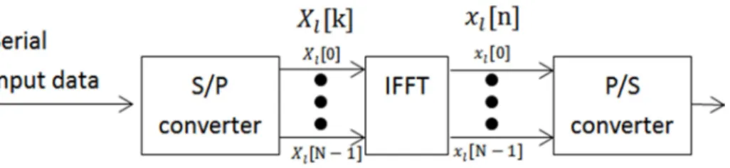
Orthogonal frequency division multiplexing (OFDM) was first proposed almost five decades ago by R. W. Chang [8]. The scheme was soon analyzed by Saltzberg [9]. The name OFDM comes from the fact that the frequency response of the subchannels are overlapping but orthogonal; its spectrum efficiency is better than traditional FDM, as depicted in Figure 2.1. Data are transmitted by parallel channels in OFDM system, so serial data should be transformed into converted data first. After we get parallel data, N-point inverse fast Fourier transform (IFFT) is taken, so as to generate samples which are sum of N orthogonal sub-carrier signals. These subsub-carriers can be defined

Φk(t) = ej2πfkt = ej2πk∆f t = ej

2πkt

Tsym_{, k = 0, 1, ..., N − 1,} _(2.1)

where fk denotes the frequency of the kth subcarrier, ∆f denotes subcarrier spacing and

Tsymdenotes OFDM symbol duration. These subcarriers are orthogonal because the integral

of their pairwise products over a symbol period is zero, that is,

Z _T_sym 0 Φk(t)Φ∗i(t)dt = Z _T_sym 0 ejTsym2πkte−j 2πit Tsymdt = Z _T_sym 0 ej2π(k−i)tTsym = ½ Tsym, if k = i, 0, if k 6= i. (2.2) 6

(22)

Figure 2.2: A baseband equivalent illustration of modulation in an OFDM system. The transmitted signal, which are referred to as OFDM symbols, are produced by combining data subcarriers. The transmitted signal is given by

xl(t) = ∞ X l=0 N −1_X k=0 Xl(k)Φk(t) = ∞ X l=0 N −1_X k=0 Xl(k)ej 2πkt

Tsym, lT_sym < t 6 (l + 1)T_sym, (2.3)

where xl(t) denotes the lth transmit symbol at time t and Xl(k) denotes the lth transmit

symbol at the kth subcarrier. The continuous-time baseband OFDM signal in (2.3) can be

sampled at t = lTsym+nTswith Ts = Tsym/N to yield the correponding discrete-time OFDM

symbol as xl[n] = N −1 X k=0 Xl[k]ej 2πkn N for n = 0, 1, ..., N − 1. (2.4)

Note that (2.4) turns out to be the N-point IFFT of data symbols Xl(k), k = 0, 1, ..., N − 1.

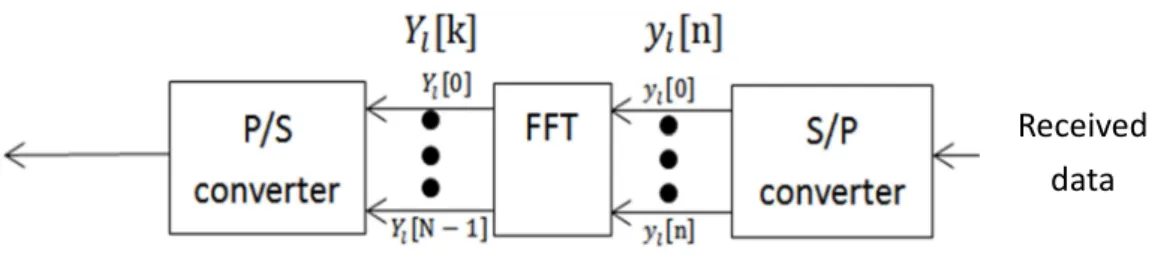
The entire process is illustrated in Figure 2.2. For demodulation, by (2.2) we can detect the data on kth subcarrier by integrating the product of the OFDM symbol and the complex conjugate of the kth subcarrier. The discrete-time version is shown in Figure 2.3 and can be expressed as Yl[k] = N −1 X n=0 yl[n]e−j2πkn/N = N −1 X n=0 ( 1 N N −1_X i=0 Xl[i]ej2πin/N ) e−j2πkn/N = 1 N N −1_X n=0 N −1_X i=0 Xl[i]e−j2π(k−i)n/N = Xl[k]. (2.5) 7

(23)

Received data

Figure 2.3: A baseband equivalent illustration of demodulation in an OFDM system.

2.1.2 OFDMA

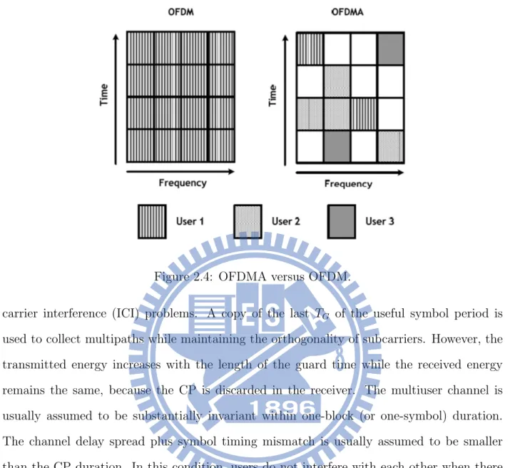
In general, OFDM is a transmission technique in which all subcarriers are used for trans-mitting the symbols of a single user. Although OFDM is not a multiple access technique by itself, it can be combined with existing multiple access technique such as TDMA (time division multiple access), FDMA (frequency division multiple access), and CDMA (code di-vision multiple access) for a multiuser system. We only treat OFDMA because it is used in LTE and LTE-A.

As depicted in Figure 2.4, the OFDMA system assigns a subset of subcarriers to each user, where the number of subcarriers of a specific user can be adaptively varied in each symbol. As users in the same cell may have different signal-to-noise ratios (SNRs), it would be more efficient to allow the multiple users each uses a subset of subcarriers with a better channel condition, rather than let a single user use all subcarriers at one time. Improvement in the bandwidth efficiency with the former condition is referred to as multiuser diversity gain. OFDMA is a technique that can leverage the multiuser diversity gain inherent to the multicarrier system.

2.1.3 Cyclic Prefix

Cyclic prefix (CP), a copy of the last part of the OFDMA symbol (see Fig. 2.5), is used in OFDM and OFDMA systems to overcome the intersymbol interference (ISI) and

(24)

Figure 2.4: OFDMA versus OFDM.

carrier interference (ICI) problems. A copy of the last TG of the useful symbol period is

used to collect multipaths while maintaining the orthogonality of subcarriers. However, the transmitted energy increases with the length of the guard time while the received energy remains the same, because the CP is discarded in the receiver. The multiuser channel is usually assumed to be substantially invariant within one-block (or one-symbol) duration. The channel delay spread plus symbol timing mismatch is usually assumed to be smaller than the CP duration. In this condition, users do not interfere with each other when there is proper time and frequency synchronization. As depicted in Figure 2.6, CP is added before transmission to generate sl[n]. After passing through the channel hl[n], white Gaussian noise

zl[n] is added. Thus the received signal is given by

rl[n] =

∞ X m=0

hl[m]sl[n − m] + zl[m]. (2.6)

After removing CP, the received samples rl[n] become yl[n], n = 0, 1, ..., N − 1, whose FFT

is given by

(25)

TG Tsub

Cyclic prefix (CP)

th OFDM symbol

Tsym

Figure 2.5: OFDM symbols with CP.

Figure 2.6: OFDM baseband transmission system structure.

(26)

Yl[k] = N −1_X n=0 yl[n]e−j2πkn/N = N −1_X n=0 ( ∞ X m=0 hl[m]xl[n − m] + zl[n] ) e−j2πkn/N = 1 N N −1_X i=0 (( _∞ X m=0 hl[m]e−j2πim/N ) Xl[i] ∞ X n=0 e−j2π(k−i)n/N ) e−j2πkn/N + Zl[k] = Hl[k]Xl[k] + Zl[k], (2.7)

where Xl[k], Yl[k], Hl[k] and Zl[k] denote the kth subcarrier frequency response of the lth transmitted symbol, received symbol, channel frequency response and noise in the frequency domain, respectively. From the last equality in (2.7), we can find that the OFDM system can be regarded as simply multiplying the input symbol by the channel frequency response in the

frequency domain. Since Yl[k] = Hl[k]Xl[k] in absence of noise, the transmitted symbol at

each subcarrier can be recovered by one-tap equalization, which simply divides the received

symbol by the channel frequency response to recover the transmitted data, i.e., ˆXl[k] =

Yl[k]/Hl[k] where ˆXl[k] denotes the equalized signal value. Note that Yl[k] 6= Hl[k]Xl[k]

without CP, since F F T {yl[n]} 6= F F T {xl[n]}·F F T {hl[n]} when yl[n] = xl[n]∗hl[n], where ∗

denotes convolution. Insertion of CP in the transmitted signal makes it circularly convolved

with the channel impulse response, i.e., yl[n] = xl[n] ⊗ hl[n], where ⊗ denotes circular

convolution, which yields Yl[k] = Hl[k]Xl[k] as desired in the receiver.

2.2 Frame Structure in LTE

The contents of this section are mainly taken from [6].

Throughout the specification for frame structure in LTE, the size of various fields in the

time domain (TD) is normally expressed in time units of Ts = 1/(15000 × 2048) seconds.

DL and UL transmissions are organized into radio frames with frame duration that equals

Tf = 307200 × Ts = 10 ms. Frame structure type 1, which applies to both full duplex and

(27)

Figure 2.7: Frame structure type 1 [7, Figure 8.2].

half duplex FDD, is shown in Figure 2.7. There are 20 slots in a radio frame with length

Tslot= 15360 × Ts= 0.5 ms, numbered from 0 to 19. A subframe consists of two consecutive

slots where subframe i consists of slots 2i and 2i + 1. For FDD, there are 10 subframes for both DL and UL transmissions in each 10 ms interval, where UL and DL transmissions are separated in the frequency domain. In half-duplex FDD operation, the UE cannot transmit and receive at the same time while there are no such restrictions in full-duplex FDD.

A resource block (RB) is defined as NRB

SC consecutive subcarriers in the FD and NsymbDL

OFDM symbols in the DL or NU L

symb SC-FDMA symbols in the UL. An RB therefore consists

of NRB

SC × NsymbDL resource elements in the DL and NSCRB× NsymbU L resource elements in the UL.

This corresponds to 180 kHz of bandwidth in the FD and one slot in the TD. The overall transmission bandwidth parameters and RB parameters are listed in Table 2.2. The number

(28)

Table 2.2: Bandwidth Parameters and RB Parameters [6, Table 8.1]

Channel bandwidth(MHz) 1.4 3 5.0 10.0 15.0 20.0

Resource block (RB) bandwidth (kHz) 180

Number of available RBs (NDL

RB) 6 15 25 50 75 100

Number of subcarriers 72 180 300 600 900 1200

Table 2.3: RB Parameters [6, Table 5.2.3-1]

Configuration NRB sc NsymbDL NsymbU L Normal CP ∆f = 15 kHz 12 7 7 Extended CP ∆f = 15 kHz 12 6 6 ∆f = 7.5 kHz 24 3 NA of subcarriers within an RB, NRB

SC, is 12 or 24 for the case of 15 or 7.5 kHz subcarrier

spacing respectively, as shown in Table 2.3. Each element in the resource grid is called a resource element (RE) and is uniquely defined by the index pair (k, l) in a slot where

k = 0, ..., NU L

RB·NscRB−1 and l = 0, ..., NsymbU L −1 are the indices in the FD and TD, respectively.

RE (k, l) corresponds to the complex signal value ak,l. For an RE not used for transmission

of a physical channel or a physical signal in a slot, ak,l is set to zero. The relation between

the RB index nRB in the FD and RE (k, l) in a slot is given by

nRB = b

k

NRB

sc

c.

Figure 2.8 shows the detailed slot structure. We focus on the case of normal CP. The normal

CP length is 5.2 µs (160 × Ts) in the first OFDM or SC-FDMA symbol and 4.7 µs (144 × Ts)

in the remaining six symbols. The overhead for the normal CP setup is about 7.14%.

2.3 Downlink Distributed Transmission

The contents of this section are mainly taken from [7]. 13

(29)

Figure 2.8: Slot structure for normal and extended CP [7, Fig. 8.3].

In the LTE DL transmission, the virtual resource block (VRB) concept is defined to enable distributed transmission. The size of VRB is same as RB. There are two types of VRBs, one is localized type, the other is distributed type. For each type of VRBs, a pair of VRBs over

two time slots in a subframe is assigned together by a single virtual block number, nV RB.

In localized type, VRBs are mapped to RBs directly, namely nRB = nV RB. Furthermore,

the VRBs of localized type are numbered from 0 to NDL

V RB − 1, where NV RBDL = NRBDL. In the

distributed type, the VRBs are numbered from 0 to NDL

V RB − 1, where NV RBDL follows certain

rules. More detailed description can be found in reference [5].

2.4 General Structure for Downlink Physical Channels

The contents of this section are mainly taken from [6]. This section gives us a brief description of the general structure of various DL physical channel defined in LTE. The baseband signal representing the physical DL channel in LTE is defined in terms of the following steps and illustrated in Figure 2.9. More detailed description can be found in reference [6].

(30)

Figure 2.9: Overview of physical channel processing [6].

• Scrambling.

• Modulation of scrambled bits to generate complex-valued symbols.

• Mapping of the complex-valued modulation symbols onto one or several transmission

layers.

• Transform precoding to generate complex-valued symbols. • Precoding of the complex-valued symbols.

• Mapping of complex-valued symbols to REs.

• Generation of complex-valued time-domain OFDMA signal for each antenna port.

2.5 Reference Signal (RS)

The contents of this section are mainly taken from [7].

Three types of DL reference signals (RSs) are defined in LTE, and five types in LTE-A. They are listed below.

• Cell-specific reference signals (CRS) • MBSFN reference signals

(31)

• UE-specific reference signals (DM-RS)

• Positioning reference signals (PRS) (LTE-A only) • CSI reference signals (CSI-RS) (LTE-A only)

In this thesis, we concentrate on the cell-specific RSs.

2.5.1 Cell-Specific Reference Signals (CRS)

Cell-specific reference signals are transmitted in all DL subframes in a cell supporting non-MBSFN transmission, and are transmitted on one or several of antenna ports 0 to 3. Note

that CRSs are defined for 4f = 15 only. The CRS sequence rl,ns(m) is defined as

rl,ns(m) = 1 √ 2(1 − 2 · c(2m)) + j 1 √ 2(1 − 2 · c(2m + 1)), m = 0, 1, ..., 2N DL P RB− 1, (2.8)

where ns and l are the slot number within a radio frame and the OFDM symbol number

within the slot respectively. The pseudo-random sequence (PN sequence) is a Gold sequence composed of two sequences of length 31, which are initialized with

cinit(m) = 210· (7 · (ns+ 1) + l + 1) ·

¡

2 · N_IDcell+ 1¢+ 2 · 2 · N_IDcell+ NCP, (2.9)

at the start of each OFDM symbol where Ncell

ID is the cell identity and NCP = 1 and 0 for

normal and extended CP, respectively. The sequence c(m) is defined by

c(m) = (x1(m + 1600) + x2(m + 1600)) mod 2 (2.10)

where x1(m) and x2(m) are respectively generated by feedback polynomials D31+ D3 + 1

and D31_{+ D}3_{+ D}2_{+ D + 1 as}

x1(m + 31) = (x1(n + 3) + X1(n)) mod 2,

x2(m + 31) = (x2(n + 3) + x2(n + 2) + x2(n + 1) + X2(n)) mod 2.

(2.11)

(32)

Figure 2.10: PN sequences generation in the LTE-system [7, Fig. 9.2]. The overall PN-sequences generator is illustrated in Figure 2.10.

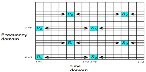
Figure 2.11 illustrates an example of the REs used for RS transmission under normal CP.

The notation RP is used to denote an RE used for RS transmission on antenna port p.

(33)

Figure 2.11: Mapping of DL RSs (normal CP) [6, Fig. 9.9].

(34)

Chapter 3 Channel Estimation Methods

Channel estimators in an OFDM or OFDMA system usually need RSs. The RS have to be transmitted continuously because a fading channel requires constant tracking. Generally speaking, the structure of the frequency response of a fading channel can be viewed as a two-dimensional (2-D) signal (frequency and time), whose values are sampled at certain positions with particular rules.

We introduce four ways of channel estimation in this chapter, including the least-squares (LS) technique, interpolation schemes, basis expansion model (BEM) with discrete prolate spheroidal sequences (DPSS), and linear minimum mean-square error (LMMSE) estimation. In the final proposal design, we use the LS technique to estimate the channel response at RSs, then use linear interpolation or BEM with DPSS in the time domain to estimate the frequency response at nonRS subcarriers within pilot symbols, and then perform LMMSE channel estimation in the frequency domain to estimate the frequency response at nonRS subcarriers within pilot symbols. Finally, we use linear interpolation or BEM with DPSS in the time domain to estimate the frequency response at nonRS subcarriers for nonpilot symbols. These building-block techniques are introduced separately in the following subsections.

(35)

3.1 Least-Squares (LS) Estimation

Based on the a priori known data, i.e., RSs, we can estimate the channel response at the RS carriers coarsely by LS estimation. Conventional LS channel estimation minimizes the squared channel estimation error based on one-sample observation [11]. Since the estimation applies to RSs in pilot symbols, we use a subscript “RS” to indicate it. The minimization objective is given by

kYRS,P − ˆHRS,P,LS · XRS,Pk2, (3.1)

where YRS,P is the received RS in pilot symbols after passing through the channel and XRS,P

is the a priori known RS in pilot symbols, both in the FD and both being M × 1 vectors and can be written as

YRS,P = [YRS,P(0) YRS,P(1) ... YRS,P(NP − 1)]T, (3.2)

XRS,P = [XRS,P(0) XRS,P(1) ... XRS,P(NP − 1)]T, (3.3)

where NP is the RS subcarrier numbers within the pilot symbol. ˆHRS,P,LS is an NP × NP

diagonal matrix as ˆ HRS,P,LS =      ˆ HRS,P,LS(0) ... 0 ... 0 HˆRS,P,LS(1) 0 ... 0 ... HˆRS,P,LS(2) ... 0 ... 0 HˆRS,P,LS(NP − 1)     . (3.4)

The LS channel estimate at RS subcarrier k, based on one observed OFDMA symbol

YRS,P only, is given by ˆ HRS,P,LS(k) = YRS,P(k) XRS,P(k) = HRS,P + Z(k)/XRS,P(k), (3.5)

where k = 0, ..., NP − 1, and Z(k) is the complex white Gaussian noise at RS subcarrier k.

(36)

3.2 Linear Interpolation

After obtaining the channel response estimates at some distributed subcarriers in frequency and in time, we may use interpolation to estimate the channel responses for the subcarriers between them. Linear interpolation is a commonly considered scheme due to its low com-plexity. It does interpolation between two known data. For example, we may use the channel information at two RS subcarriers in pilot symbols obtained by the LS estimator to estimate the channel frequency responses at the data symbols between them. We may also use linear extrapolation to estimate the responses at the data beyond the outermost RSs.

Mathematically, suppose we have two points (x1, y1) and (x2, y2) that are assumed to

satisfy a linear relation as

aX + b = Y, (3.6)

where a and b are unknown. Then we have

ax1+ b = y1, ax2 + b = y2.

We can write the equations in matrix form as · x1 1 x2 1 ¸ · a b ¸ = · y1 y2 ¸ . (3.7)

Then the unknown parameters a and b can be solved as · a b ¸ = · x1 1 x2 1 ¸−1· y1 y2 ¸ = 1 x2− x1 · y2− y1 x2y1− x1y2 ¸ . (3.8)

When the above interpolation is carried out in the TD between two pilot symbols at the same subcarrier, the idea is as illustrated in Figure 3.1.

3.3 Discrete Prolate Spheroidal Sequences (DPSS)

The contents of this section are mainly taken from [12]. 21

(37)

Figure 3.1: Illustration of linear interpolation in TD.

Slepian [13] introduced sequences which are bandlimited to the frequency domain [−vDmax, vDmax]

and furthermore most concentrated in a certain time interval of length M. The quantity

vDmax, denoting the maximum normalized Doppler bandwidth, is defined as

vDmax =

vmaxfC

c0

Tsym, (3.9)

where vmax is the maximum velocity, Tsymis the OFDM symbol duration, and c0 is the light

speed. Consider a sequence u[m] bandlimited to vDmax so that

u[m] = Z _v_Dmax −vDmax U(v)ej2πmv_dv, _(3.10) where U[v] = ∞ X m=−∞ u[m]e−j2πmv, (3.11)

while having its maximum energy concentration in an interval of length M

λ(vDmax, M ) = P_{M −1} m=0 |u[m]|2 P_∞ m=−∞|u[m]|2 . (3.12)

The solution for the optimization problems (3.12) is the discrete prolate spheroidal sequences

(38)

(DPSS). The ith DPSS ui[l, vDmax, M ] is defined as the real solution of

M −1_X l=0

sin(2πvDmax(l − m))

π(l − m) ui[l, vDmax, M ] = λi(vDmax, M )ui[m, vDmax, M], (3.13)

for i ∈ {0, ..., M − 1} and m ∈ {−∞, ..., ∞} [12]. We drop the arguments vDmax and M from

λi(vDmax, M ) below for simplicity.

The DPSS are doubly orthonormal on the infinite set {−∞, ..., ∞} , Z as well as the finite set {0, ..., M − 1} as M −1_X m=0 ui[m]uj[m] = λi ∞ X −∞ ui[m]uj[m] = δij, (3.14)

where i, j ∈ {0, ..., M − 1}. The eigenvalues λi associated with the sequences ui[m] have

following properties [12]:

• λi is near 1 for i ≤ d2vDmaxMe + 1.

• λi drops to zero rapidly for i > d2vDmaxMe + 1.

Hence the dimension of the signal space is approximately given by

D0 = d2vDmaxMe + 1. (3.15)

For the purpose of channel estimation, the index set m ∈ {0, ..., M − 1}, where m may be taken to be the OFDM symbol number. The DPSS expands the sequence H[m] by

H[m] ≈ ˜H[m] =

D−1_X i=0

ui[m]γi, (3.16)

where γi is the weighting coeffieients of the Slepian sequence, and the dimension D has the

constraints

D0 _{≤ D ≤ M.} _(3.17)

(39)

Figure 3.2: Illustration of Pk.

The weighting coefficient γi for i ∈ {0, ..., D − 1} is calculated as

γi ≈ ˆγi = M −1_X m=0 ˆ H[m]u∗ i[m], (3.18)

where ˆH[m] can be derived by the LS method at RS subcarriers.

In the LTE DL, RSs are only located at some OFDM symbols m ∈ Pk, where Pk is the

set of positions of RSs for subcarrier k. As depicted in Figure 3.2, P0 is composed by OFDM

symbol number l = 0 and l = 7 for subcarrier index k = 0. For simplicity, we consider a fixed subcarrier k and omit the index k in the next paragraph.

The orthogonality of the Slepian sequences is lost by only taking some values of m. In order to correct the loss of orthogonality, we have to introduce a matrix G as

G = X m∈P f[m]fH_[m], _(3.19) where f[m] =     u0[m] . . uD−1[m]     . (3.20) 24

(40)

The corrected ˆγ can be derived as [12] ˆ γ = G−1X m∈P ˆ H[m]f∗_[m], _(3.21) where ˆ γ =     ˆ γ0 . . ˆ γD−1     . (3.22)

Finally, we can use (3.16) to expand the sequences for m /∈ Pk.

3.4 Linear Minimum-Mean Square Error (LMMSE)

Chan-nel Estimation

The linear minimum mean square error (LMMSE) estimator uses second-order statistics about the channel and the noise to reduce the amount of noise in an existing channel estimate, such as the LS channel estimate, as

ˆ

HRS,LM M SE = RHRSHRS,P[RHRS,PHRS,P + σ

2

z(XRS,PH XRS,P)]−1HˆRS,P,LS, (3.23)

where ˆHRS,P,LS is the LS estimate vector obtained as in (3.5), σ2z is the variance of AWGN,

RHRS,PHRS,P is the autocorrelation matrix of the RS subcarriers within the same pilot symbol,

RHRSHRS,P is the crosscorrelation matrix between all subcarriers and the subcarriers with the

RSs within the same pilot symbol, and the superscript (·)H _{denotes Hermitian transpose.}

By replacing the term (XH

RS,PXRS,P) in (3.23) with its expectation E[(XRS,PH XRS,P)], the

LMMSE channel estimator in frequency domain can be represented as ˆ HRS,LM M SE = RHRSHRS,P(RHRS,PHRS,P + β SNRI) −1_H_ˆ RS,P,LS, (3.24) where β is a constant depending on the type of modulation, SN R is the average

signal-to-noise ratio and I is the identity matrix with same size as RHRS,PHRS,P.

(41)

As mentioned in chapter 1, we can approximate RHRSHRS,P and RHRS,PHRS,P by the mean

delay (τµ) and the RMS delay spread (τrms). The mean delay and the RMS delay spread are given by, respectively,

τµ= P_L−1 l=0 |αl|2l P_L−1 l=0 kαl|2 (3.25) and τrms = sP_L−1 l=0_P|αl|2(l − τµ)2 L−1 l=0 |αl|2 . (3.26)

One question here is how the time domain averaging (|αl|2) should be defined. As our

purpose is channel estimation, suppose one channel estimation is performed for K pilot symbols. Then the expectation should be an average taken over these symbols. In the extreme case of K = 1, no average should be taken, but the instantaneous channel response

in that symbol period should be used to compute τµ and τrms.

Once we get τµ and τrms, the elements of crosscorrelation matrix and autocorrelation

matrix can be defined if we assume the channel has exponential PDP. For an exponential

PDP with possibly nonzero initial delay τ0, we have

Rf(k) Rf(0) = e −j2πτ0k/N 1 + j2πτrmsk/N , (3.27)

where τ0 = τµ− τrms and N is the FFT size used in the multicarrier system.

3.4.1 Estimation of Channel Delay Parameters

Method 1 (“K”)

The material in this section is mainly taken from [2].

If we advance the channel response by (an arbitrary) τ time units, then the frequency response becomes Ha(f ) = ej2πτ f /NH(f ) = L−1 X l=0 αl(l − τ )e−j2π(l−τ )f /N. (3.28) 26

(42)

Differentiating Ha(f ) with respect to f , we get dHa(f ) df = −j2π N L−1 X l=0 αl(l − τ )e−j2π(l−τ )f /N. (3.29)

Applying Parseval’s theorem, we get D |dHa(f ) df | 2E₌ 4π2 N2 L−1 X l=0 |αl|2(l − τ )2, (3.30)

where < · > means frequency averaging. Taking average over time, we get D |dHa(f ) df |2 E = 4π2 N2 L−1 X l=0 |αl|2(l − τ )2 , J(τ ), (3.31)

where the overline · indicates time averaging. The above equations show that J(τ ) is

minimized when τ = τµ. In addition,

τ2 rms = N2_{min J(τ )} 4π2PL−1 l=0 |αl|2 . (3.32)

We can estimate τµ and τrms in this way, and it is suitable for typical pilot-aided OFDMA

systems.

Consider a system where one out of every Fs subcarriers is a RS. Later, we will see that

how Fs can be set in LTE. We can approximate dHa(f )/df by first-order difference, say,

[Ha(f + Fs) − Ha(f )]/Fs, and substitute it into (3.31). Then, we obtain

J(τ ) ≈ 1 F2 s D |ejφ_{H(f + F}_{s) − H(f )|}2E p, (3.33)

where φ = 2πτ Fs/N, f takes values only over RS frequencies, and < · >p denotes averaging

over RS subcarriers. By sampling theory, it is proper to take circular differencing over f rather than linear differencing [2]. Therefore, we approximate J(τ ) by

J(τ ) ≈ 1 F2 s D |ejφ_{H((f + F} s)%N ) − H(f )|2 E p, (3.34) 27

(43)

where % denotes modulo operation, < · >p now averages over the full number of RS

sub-carriers, and we have assumed that (f + Fs)%N is an RS subcarrier. Now let Ri be the

frequency-domain autocorrelation of the channel response as

Ri =

D

H((f + iFs)%N )H∗(f )

E

p. (3.35)

Then from (3.34) we have

J(τ ) ≈ 2

F2

s

[R0− R{ejφR1)}]. (3.36)

Thus (3.36) gives an approximation of J(τ ). According to (3.36), τµ and τrms can be

esti-mated in the following way:

1. estimate the channel responses at the RS subcarrier,

2. estimate Ri (i = 0, 1),

3. estimate J(τ ),

4. find the value of τ that minimizes J(τ ),

5. substitute the min J(τ ) into (3.32) to estimate τ2

rms, and

6. estimate τ0.

Step 1 can be achieved using the LS method. Then, in step 2, R0 and R1can be estimated

via ˆ R0 = D | ˆH(f )|2 E p− ˆσ 2 n, Rˆ1 = D ˆ H(f + Fs%N) ˆH∗(f ) E p, (3.37)

where ˆH(f ) denotes the estimated channel response at RS subcarrier f and, we may obtain

the noise power ˆσ2

n from the received power in the null subcarriers of the system. Thus, for

step 3, J(τ ) can be estimated using ˆ J(τ ) , 2 F2 s h ˆ R0− R{ejφRˆ1} i . (3.38) 28

(44)

If one performs a channel estimation over K pilot symbols, then the averages should be taken over these K symbols. If K = 1, then the instantaneous values should be used instead of averages. For step 4, we may estimate the mean delay as

ˆ

τµ, arg min ˆJ(τ ) = −

N∠ ˆR1

2πFs

, (3.39)

which also yields min ˆJAv(τ ) = 2[ ˆR0 − | ˆR1|]/Fs2. For step 5, in view of (3.32) and that

R0 =< |H(f )|2 >p, we may estimate τrms as ˆ τrms = N 2πFs v u u t2h1 −| ˆR1| ˆ R0 i . (3.40)

Finally, the initial delay τ0 can be estimated via

ˆ

τ0 = ˆτu− ˆτrms. (3.41)

Method 2 (“Y”)

Recall (3.27). We can get

Rf(k)

Rf(0)

× (1 + j2πτrmsk/N) = e−j2πτ0k/N. (3.42)

For convenience, let

R = Rf(k) Rf(0) (3.43) and X = 2πτrmsk N . (3.44)

Substituting (3.43) and (3.44) into (3.42) yields

R × (1 + jX) = e−j2πτ0k/N_. _(3.45)

Taking the squared magnitudes of both sides of (3.45) yields

1 = |R × (1 + jX)|2

= (R(R) − I(R)X)2_{+ (I(R) − R(R)X)}2

= (R(R)2_{+ I(R)}2_{)(1 + X}2_).

(3.46)

(45)

To solve for X, we rewrite (3.46) as X2 ₌ 1 R(R)2 _{+ I(R)}2 − 1 = Rf(0)2 R(Rf(k))2_{+ I(Rf}_(k))2 − 1. (3.47)

The above equation have several unknowns, which are k and Rf(k). As in method 1, we

can replace k by Fs for a system where one out of every Fs subcarriers is a RS. The other

unknown Rf(k) can be derived by (3.37), too. As a result, we get from (3.44) and (3.47)

that ˆ τrms = N 2πFs v u u t Rˆ0 2 R( ˆR1)2+ I( ˆR1)2 − 1. (3.48)

We substitute the result back to (3.42). Finally, we may estimate τ0 by

ˆ τ0 = −∠(Rˆ1 ˆ R0 × (1 + j2πˆτrmsFs/N)) 2πFs/N . (3.49)

3.5 Improving the Accuracy of the Estimated Channel

Parameters

The question which we must consider is accuracy of our estimated channel parameters. In an LTE system, the distance between adjacent CRSs in the frequency domain is 6 subcarriers or 90 kHz, which is on the order of coherence bandwidths of outdoor channels that have middle to large spreads. To improve the accuracy of the estimated channel parameters, shorten the distances between adjacent RSs can be considered. However, the distance is set by LTE which we cannot violate, so we consider producing “pseudo” RR by linear interpolation or use of BEM with DPSS in TD of channel response estimates at the RS subcarriers in some

other pilot symbols. The idea is illustrated in Figure 3.3, where R0 is channel response at

the RS subcarriers, and P0 is a pseudo RR that is estimated via linear interpolation or BEM

with DPSS. The pseudo RR can be treated similarly as the original channel response at the 30

(46)

Figure 3.3: Illustration of pseudo RR.

RS subcarriers in channel estimation, which makes the distance between adjacent RSs in the FD reduced. In Figure 3.3, the distance between adjacent RSs in the FD is 6 originally, but now can be made to equal 3.

3.5.1 Channel Estimation Flow

With the idea of producing pseudo RR, the overall channel estimation flow is depicted in

Figure 3.4. In Figure 3.4(a), we use the LS in FD to estimate RSs then we get R0. In

Figure 3.4(b), we produce some P0 by linear interpolation or use of BEM with DPSS in

TD of channel response estimates at the RS subcarriers in some other pilot symbols. In

Figure 3.4(c), the channel delay parameters can be estimated via R0 and P0. The estimated

channel delay parameters can be substituted into proper places in (3.27) then the resulting autocorrelation function and crosscorrelation function of channel frequency response can be used in the LMMSE channel estimate. Note that we only use the LMMSE method in FD, thus we can get other data, denoted as D, only in pilot symbols. In Figure 3.4(d), we estimate remaining data signals via linear interpolation or use of BEM with DPSS in TD of

(47)

a b

c d

Figure 3.4: Channel estimation flow with use of pseudo RR.

(48)

channel response estimates at the data subcarriers in notpilot symbols.

(49)

Chapter 4 Simulation of LTE Downlink Channel

Estimation

In this chapter, we take the LMMSE approach described in the last chapter to do LTE DL channel estimation. We evaluate the performance of different ways of channel estimation quantitatively using the mean square error (MSE) and symbol error rate (SER).

4.1 Simulation Conditions

The system parameters used in our simulation are listed in Table 4.1. In addition to AWGN which is for calibration purpose, we also simulate SUI-2 (where SUI stand for Stanford Uni-versity Interim),SUI-4, SUI-5, TU (Typical Urban) [10], ITU-VA (International Telecommu-nication Union RadiocommuTelecommu-nication Vehicular A), and an artificial channel model based on ITU-VA [2]. The SUI channels model deal suburban path loss environments in three different types, depending on the tree density and pass loss condition. The three types in suburban area are listed in Table 4.2. SUI1 and SUI2 are Rician multipath channels and the other four are Rayleigh multipath channels; the former two correspond to situations with line-of-sight (LOS) and the latter four non LOS respectively. The Rayleigh channels are more hostile and exhibit a greater root-mean-square (RMS) delay spread. In our simulation, we employ

(50)

Table 4.1: OFDMA Downlink Parameters (Normal CP)

Parameters Values

Bandwidth [MHz] 5 / 10

modulation type QPSK

Central frequency [GHz] 2

Number of resource blocks 25 / 50

Number of occupied subcarriers 300 / 600

CP time [µs] (first symbol in slot, else) 5.2, 4.7

NF F T 512/1024

Sampling frequency [MHz] 7.68 / 15.36

Subcarrier spacing [kHz] 15

Symbol time [µs] (first symbol in slot, else) 71.8, 71.3

Samples per slot 3840 / 7680

three types of environments, i.e., terrain A, B, and C. We select SUI-2, SUI-4, and SUI-5 as representative for terrain C, terrain B, and terrain A, respectively. For simplicity, we use Rayleigh fading to model SUI-2 instead of Rician fading.

The TU channel model, as its name shows, is a channel model for the urban environment. The TU channel model is also a Rayleigh channel, but there are 12 taps in it, which is four-times that of SUI channels. The ITU-VA is a channel model for UE in vehicular type of motion. The ITU-VA channel model is a Rayleigh channel. There are 6 taps in it, which is two-times that of SUI channels. In order to see how the proposed technique may perform in various conditions, we choose these quite different channel models to do our simulation. Artificial ITU-VA [2], the PDP of which is far from exponential PDP, is also chosen to see how the proposed technique may perform when the PDP is totally different from exponential PDP. The PDP of the artificial ITU-VA consists of three copies of ITU-VA’s PDP with intercluster delays of 2 and 4 µs, respectively. The relative power scales of three clusters are 0, 5, and −2 dB, respectively. It has been shown that exponential PDP modeling performs better than uniform modeling [2] when the PDP is Artificial ITU-VA. But the performance is unknown for exponential PDP modeling in the method described in chapter 3. We thus

(51)

Path gain 0 1 2 3 Sample index Adjustment required Adjustment required

Figure 4.1: Tap adjustment.

Table 4.2: SUI Channel Model for Differetn Terrain Types

Terrain type Description SUI channels

A hilly terrain with heavy tree SUI5, SUI6

B flat terrain with heavy tree, hilly

terrain with light tree

SUI3, SUI4

C flat terrain with light tree SUI1, SUI2

simulate this channel model to understand it.

Tables 4.3–4.8 present the characteristics of the models mentioned above. Note that the PDP of each channel model may not have the path delays equal to integer multiples of the LTE sample spacing. Experience with the Matlab channel simulator shows that this situation results in huge amount of memory usage which causes difficulty in simulation of systems where the FFT size is more than 512. To solve this problem, the PDP listed in Table 4.4–4.8 are adjusted by forcing each channel impulse response tap to its nearest sampling point by rounding to preserve the path number as well as path power. The idea is illustrated in Figure 4.1. Expeiments show that the performance with and without tap adjustment is almost the same.

(52)

Table 4.3: PDP of SUI2

Relative delay Average power

Tap µs sample numbers

(512,1024) dB normalized dB 1 0 (1, 1) 0 −0.393 2 0.4 (4, 7) −12 −12.393 3 1.1 (9, 18) −15 −15.393 Table 4.4: PDP of SUI4

(512,1024) dB normalized dB 1 0 (1, 1) 0 −1.9218 2 1.5 (13, 24) −4 −5.9218 3 4 (32, 62) −8 −9.9218 Table 4.5: PDP of SUI5

(512,1024) dB normalized dB 1 0 (1, 1) 0 −1.5113 2 4 (32, 62) −5 −6.5113 3 10 (78, 155) −10 −11.5113

4.1.1 Parameter Setting

We now discuss considerations concerning tap number of LMMSE filtering, length of DPSS, time-bandwidth product, and number of DPSS bases.

It is known that the coherent bandwidth, denoted as Bc herein, is inversely proportional

(53)

Table 4.6: PDP of TU

(512,1024) dB normalized dB 1 0 (1, 1) −4 −10.3582 2 0.1 (2, 3) −3 −9.3582 3 0.3 (3, 6) 0 −6.3582 4 0.5 (5, 9) −2.6 −8.9582 5 0.8 (7, 13) −3 −9.3582 6 1.1 (9, 18) −5 −11.3582 7 1.3 (11, 21) −7 −13.3582 8 1.7 (14, 27) −5 −11.3582 9 2.3 (19, 36) −6.5 −12.3582 10 3.1 (25, 49) −.6 −14.9582 11 3.2 (26, 50) −11 −17.3582 12 5.0 (39, 78) −10 −16.3582 Table 4.7: PDP of ITU-VA

(512,1024) dB normalized dB 1 0 (1, 1) 0 −3.14 2 0.31 (3, 6) −1 −4.14 3 0.71 (6, 12) −9 −12.14 4 1.09 (9, 18) −10 −13.14 5 1.73 (14, 28) −15 −18.14 6 2.51 (20, 40) −20 −23.14

to the RMS delay spread denoted τrms, that is [10],

Bc ∝ 1

τrms

. (4.1)

The proportionality constant in (4.1) may vary with the definition of coherence bandwidth or other considerations. For instance, if the coherence bandwidth is defined as bandwidth

(54)

Table 4.8: PDP of Artificial ITU-VA

(512,1024) dB normalized dB 1 0 (1, 1) 0 −9.95 2 0.31 (3, 6) −1 −10.95 3 0.71 (6, 12) −9 −18.95 4 1.09 (9, 18) −10 −19.95 5 1.73 (14, 28) −15 −24.95 6 2 (16, 32) 5 −4.95 7 2.31 (19, 36) 4 −5.95 8 2.51 (20, 40) −20 −29.95 9 2.71 (22, 43) −4 −13.95 12 3.09 (25, 48) −5 −14.95 11 3.73 (30, 58) −10 −19.95 12 4 (32, 62) −2 −11.95 13 4.31 (34, 67) −3 −12.95 14 4.51 (36, 70) −15 −24.95 15 4.71 (37, 73) −11 −20.95 16 5.09 (40, 79) −12 −21.95 17 5.73 (45, 89) −17 −26.95 18 6.51 (51, 101) −22 −31.95

Table 4.9: RMS Delay of Channel after Tap Adjustment with FFT size = 512

Channel Model SUI-2 SUI-4 SUI-5 TU ITU-VA Artificial

ITU-VA RMS delay spread (sample) 1.485 9.794 21.92 7.905 2.726 9.437 RMS delay spread (µs) 0.193 1.275 2.854 1.03 0.355 1.229

with correlation of 0.9 or above in channel frequency response, then we have

Bc≈

1

50τrms. (4.2)

In case the coherence bandwidth is defined as bandwidth with correlation of 0.5 or above in 39

(55)

channel frequency response, it is given as

Bc≈

1

5τrms

. (4.3)

Here we consider the latter definition. In this case, if τrms is equal to 2 µs, which is a

relatively large RMS delay spread, then the coherence bandwidth is equal to 100 kHz. On

the other hand, if τrms is equal to 0.2 µs, which is a relatively small RMS delay spread, then

the coherence bandwidth is equal to 1 MHz. The use of pseudo RR as discussed in chapter 3 makes the spacing between adjacent RSs equal to 45 kHz in LTE and LTE-A. Considering both the large and small RMS delay spread environments, it appears that 4 is a proper number of LMMSE filter taps.

Now consider the other parameters, namely, length of DPSS, time-bandwidth product, and number of DPSS bases. We may intuitively expect that a longer length of the DPSS should result in better performance. But longer DPSS imply grater latency and grater mem-ory requirement. We let it be 7 slots plus 1 symbol, i.e., about 3.6 ms in our simulation, which is a relatively arbitrary choice. The time-bandwidth product is related to the nor-malized Doppler frequency, which is not estimated in this thesis. But as shown in (3.15), the product has to be rounded in determining the dimensions used, which means there is a high tolerance to error in the assumed normalized Doppler frequency. Our simulation results show that DPSS for higher normalized Doppler frequencies can be used in cases with lower normalized Doppler frequencies with some small degradation. Thus we choose a set that corresponds to about 150–300 km/h for the 0-300 km/h operating environment when the carrier frequency is equal to 2 GHz. The number of DPSS bases, where each basis sequence corresponds to a different eigenvalue, is determined by simulation. We find that eigenvalues lower than 0.001 can be discarded with little degradation. And the lowest eigenvalue should be in the interval [0.01, 0.001] for the best performance. So here we preserve 7 DPSS bases, where the 7th eigenvalue is 0.0034 and the 8th is 0.00018.

(56)

4.2 Simulation Results for LTE

In our simulation, we assume perfect synchronization. We also assume that the channels are block-static, i.e., they have constant responses within one symbol duration.

Because we simulate many different ways of channel estimation, each figure will contain many lines. We here give a brief outline of the different methods and how their corresponding results are indicated in the figures. There are 16 lines in each figure, each line representing a certain method. The lines are named ALS, Interp, PerPL, KML, YML, YD-MA, KD-MA, YDMD, KDMD, YDML, KDML, PerPD, YL-KD-MA, KL-KD-MA, YLML and KLML. ALS means perfect condition. where all subcarriers in all symbols are RSs. This condition is used as a reference condition for performance comparison. PerP is similar to ALS, the only difference being that all subcarriers are RSs in pilot symbols only. “L” means doing linear interpolation/extrapolation in time domain. “K” and “Y” are method 1 and method 2, respectively, as introduced in Section 3.4.1, which are different methods to estimate the channel delay parameters. “D” means using BEM with DPSS in TD. “M” means doing LMMSE estimation in FD on pilot symbols only, whereas “MA” means doing LMMSE estimation in FD on all symbols.

A brief describtion of the various different methods are as follows. 1) ALS:

• Estimate the channel response at each subcarriers by the LS technique.

2) PerPL and PerPD:

• Estimate the channel response at each RS location by the LS technique. • Do linear interpolation/extrapolation or BEM with DPSS in time domain.

(57)

3) Interp:

• Estimate the channel response at each RS location by the LS technique. • Do linear interpolation/extrapolation in frequency domain.

• Do linear interpolation/extrapolation in time domain.

4) KML and YML:

• Estimate the channel response at each RS location by the LS technique. • Estimate the channel delay parameters by method K or Y on pilot symbols. • Do LMMSE channel estimation in the frequency domain for pilot symbols. • Do linear interpolation/extrapolation in time domain.

5) KD-MA, YD-MA, KL-MA, and YL-MA:

• Estimate the channel response at each RS location by the LS technique.

• Do linear interpolation/extrapolation or BEM with DPSS in time domain to create

pseudo RR on all symbols.

• Estimate the channel delay parameters by method K or Y for all symbols. • Do LMMSE channel estimation in the frequency domain on all symbols.

6) KDMD, YDMD, KDML, YDML, KLML, and YLML:

• Estimate the channel response at each RS location by the LS technique.

• Do linear interpolation/extrapolation or BEM with DPSS in time domain to create

pseudo RR on pilot symbols.

運用功率延遲輪廓近似之線性最小均方差通道估計於LTE下行時變通道傳輸

國 立 交 通 大 學

電子工程學系 電子研究所碩士班

碩 士 論 文

運用功率延遲輪廓近似之線性最小均方差通道估

計於 LTE 下行時變通道傳輸

LMMSE Channel Estimation with Power-Delay

Profile Approximation for LTE Downlink

Transmission over Time-Variant Channels

研 究 生 ： 楊葆崧

指導教授 ： 林大衛 教授

運用功率延遲輪廓近似之線性最小均方差通道估

計於 LTE 下行時變通道傳輸

LMMSE Channel Estimation with Power-Delay

Profile Approximation for LTE Downlink

Transmission over Time-Variant Channels

研 究 生：楊葆崧 Student: Bao-Song Yang

指導教授：林大衛 Advisor: Dr. David W. Lin

國 立 交 通 大 學

電子工程學系 電子研究所碩士班

碩 士 論 文

運用功率延遲輪廓近似之線性最小均方差通道估

計於 LTE 下行時變通道傳輸

研究生：楊葆崧 指導教授：林大衛 博士

國立交通大學

電子工程學系 電子研究所碩士班

摘要

LMMSE Channel Estimation with Power-Delay

Profile Approximation for LTE Downlink

Transmission over Time-Variant Channels

Student: Bao-Song Yang Advisor: Dr. David W. Lin

Department of Electronics Engineering

Institute of Electronics

National Chiao Tung University

Abstract

誌謝

Contents

List of Figures

List of Tables

Chapter 1

Introduction

1.1

Contributions

Chapter 2

Overview of LTE and LTE-A

Downlink Specifications

2.1

Overview of OFDM and OFDMA

2.1.1

OFDM

2.1.2

OFDMA

2.1.3

Cyclic Prefix

2.2

Frame Structure in LTE

2.3

Downlink Distributed Transmission

2.4

General Structure for Downlink Physical Channels

2.5

Reference Signal (RS)

2.5.1

Cell-Specific Reference Signals (CRS)

Chapter 3

Channel Estimation Methods

3.1

Least-Squares (LS) Estimation

3.2

Linear Interpolation

3.3

Discrete Prolate Spheroidal Sequences (DPSS)

3.4

Linear Minimum-Mean Square Error (LMMSE)

Chan-nel Estimation

3.4.1

Estimation of Channel Delay Parameters

3.5

Improving the Accuracy of the Estimated Channel

Parameters

國立交通大學

電子工程學系電子研究所碩士班

碩士論文

研究生：楊葆崧

指導教授：林大衛教授

研究生：楊葆崧 Student: Bao-Song Yang

國立交通大學

電子工程學系電子研究所碩士班

碩士論文

研究生：楊葆崧指導教授：林大衛博士

電子工程學系電子研究所碩士班