霍爾感應器用於近場磁感應通訊之探討

(1)

國立交通大學

電子工程學系電子研究所碩士班

碩士論文

霍爾感應器用於近場磁感應通訊之探討

Research on Hall sensors applied to Near-field Magnetic Induction

Communication

研究生 : 沈資偉

指導老師 : 桑梓賢教授

(2)

I

霍爾感應器用於近場磁感應通訊之探討

研究生：沈資偉指導教授：桑梓賢教授

國立交通大學

電子工程學系電子研究所碩士班

摘要

隨著電信的發展與進步，現今的無線通訊有向物聯網發展的趨勢。但物聯網的多種應用同時也帶來了許多挑戰，舉例來說，低能量消耗，高資料傳輸量，和較小的體積設計。對物聯網來說，如何選擇一個近距離的物理層傳輸技術如射頻識別技術(Radio-Frequency identification)RFID，跟近場磁通訊(Near Field Magnetic Induction Communication )NFMIC 是很重要的。

在一些要考慮溼度，土壤，人體組織…等的通道環境下，NFMIC 的獨特性質使其有比 RFID 更好的表現。在 NFMIC 系統中，使用線圈來產生磁場以傳輸資訊。但由於線圈的特性，如果想要得到較大的傳輸磁場，就需要更多圈數，如此一來線圈的體積就會變大，這並不適合用於產品上。因此我們使用霍爾感應器(Hall sensor)替換接收端的線圈使體積縮小，由於霍爾感應器的輸出電壓是由磁場的變化跟偏壓的電流所影響，所以它有比線圈更小的體積，但同時也要付出一些效能上的代價，本篇論文會分析為了更小的體積會付出哪些代價。論文的結構如下所示：第一章介紹物聯網，近場磁通訊與霍爾感應器。第二章提出使用線圈和霍爾感應器的兩種近場磁通訊系統模型。第三章規劃系統的需

(3)

II

求及規格，並且說明如何處理記錄的資料。第四章比較量測到的資料與理論上推導的資料，並近一步比較訊雜比，通道容量。最後總結這個方法並且討論未來發展的方向和可行的運用。

(4)

III

Research of Hall sensors applied to Near-field Magnetic

Induction Communication

Student: Tzu-Wei Shen

Advisor: Tzu-Hsien Sang

Department of Electronics Engineering & Institute of

Electronics National Chiao Tung University

Abstract

There is a recent trend of Internet of Things (IOT) in modern wireless

communications. Due to the various applications in IOT, there are many challenges, too. (e.g., low power consumption, high data rates, and the small volume). Because many applications of IOT are used in short-distance wireless communication. Thus, choosing a suitable wireless communication method in short distance is very

important. For instance, Radio-Frequency identification (RFID) is suitable for air medium, and Near Field Magnetic Induction Communication (NFMIC) is suitable for non-air media.

In Comparison with RFID, unique characteristics of NFMIC particularly make it more suitable than RFID in some circumstance, where the communication

environment consists of humidity, soil or body organs. In NFMIC system, coils are usually needed to generate the magnetic field to transmit signals. According to the property of coil, if we want to produce a bigger magnetic field, the coil needs more turns. In this way, the volume of coil will increase, and it is not desirable.

(5)

IV

Hall sensors have smaller volume than coils, and it can replace coils in the receiver to reduce the volume of receiver. The working principle of Hall sensors is generating voltage by Hall Effect to sense the changes of magnetic fields. However, there is a tradeoff between performance and volume. In this study, the costs of small volume consist of low capacity, short available transmission distance and bad signal to noise ratio…etc. .

This paper is organized as follows. Chapter 1 introduces the Internet of things (IOT), near field magnetic induction communication (NFMIC) and Hall sensors. Chapter 2 proposes two system models; the near field magnetic induction

communication system and Hall sensor based system. Chapter 3 lays out system requirements and specifications, and presents how the experiment is conducted. Then Chapter 4 compares experimental and theoretical results. Furthermore, we also compare the signal to noise ratio, and channel capacities. In the end, we summarize this thesis and propose future work directions and possible applications in Chapter 5.

(6)

V

誌謝

首先，我要先感謝指導教授桑梓賢-老師。謝謝老師在一路懵懵懂懂的研究之路上，包容各種愚昧的問題並且耐心地指導，從老師的身上學到了如何思考問題的邏輯和方向，使我在遇到問題時能更有效率的解決它；除此之外，也會分享一些人生智慧給我們當作前車之鑑，而對於世界上的國際大事，也會分享他的觀點給我們做為參考，相信這些寶貴的經驗會讓我在往後的日子裡更加地受用無窮。再來我要感謝蔡嘉明教授，在我研究上給予的幫助，無論是一些研究上相關的問題，或是研究主題方向上的探討，甚至一些測量結果上的意見都非常精闢，在此特別感謝。還有一直幫忙測量數值的王培宇學長，與解答了不少電路問題的沈易弘學長。這兩位學長在我的研究上也幫助了我非常多的部分，非常感謝這兩位學長的幫忙。也很感謝實驗室的同學彥凱，偉生，昀楷，唯丞，柏佾，建誠，敬昆，育綸，佳佑，文郎，欣哲，以及最厲害的志堯學長大家從碩一開始痛苦的修著課，寫完了一大堆的 project,到了碩二也各種努力的一起做研究，互相討論研究內容，也彼此再研究之路上互相的砥礪，平日的嘻笑打鬧都將再我心中留下難忘的回憶。最後，要感謝我的父母。一路以來沒有給予我太沉重的壓力與企盼，只求凡事盡力的態度，謝謝你們成為我強大的後盾，讓我在從小到大十餘年的求學生涯中無後顧之憂，能平穩順利的完成學業。

(7)

VI

List of Table

Table 1. Parameters of the transmitter ... 27

Table 2. Parameters of the receiver in coils system ... 28

Table 3. Parameters of the receiver in Hall Effect sensor systems ... 29

List of Figures

Figure 1 . Internet of Things [5] ... 2

Figure 2 . The concept of coil transmission [6] ... 3

Figure 3 . Circular Coil model [11] ... 7

Figure 4 . Equivalent circuit model of NFMIC system [11] ... 7

Figure 5 Hall Effect diagram [17] ... 14

Figure.6 Equivalent circuit model of Hall sensor based NFMIC system .... 16

Figure 7. Configuration and the dimension of the coil SPEC [19] ... 22

Figure 8. Characteristics of the coil [19] ... 23

Figure 9. Part material identification ... 23

Figure 10. RI 1020-701K ... 23

Figure 11. Features of the WSH202 [20] ... 24

Figure 12. Equivalent circuit model and OUT vs Magnetic field [20] ... 25

Figure 13. Absolute maximum rating of WSH202 [20] ... 25

Figure 14. Electrical characteristics of WSH202 [20] ... 25

Figure 15. WSH202 ... 26

Figure 16. Package information of WSH202, TO94 [20] ... 26

Figure 17. Coils system... 28

Figure 18. Hall Effect sensor system ... 29

Figure 19. Block diagram of recording signals ... 30

Figure 20.steps of recording noise ... 31

Figure 21. Coil system simulation model in PSPICE ... 35

Figure 22. Simulation of Received current in PSPICE ... 36

Figure 23. Comparing result of equation (8) and PSPICE... 36

Figure 24. Received power of coil system ... 37

Figure 25. Received power of coil system (zoom in) ... 38

Figure 26.Power transfer function of Hall Effect sensor system. ... 39

Figure 27. The noise N1 of oscilloscope. ... 40

(10)

IX

Figure 29. The noise of the oscilloscope and coil system ... 42

Figure 30. Power received versus distance ... 43

Figure 31. SNR of recorded data. ... 45

Figure 32. Compared the revised channel capacity ... 46

(11)

1

Chapter 1 Introduction

1.1 Background of Internet of things

The Internet of Things (IoT) is a novel paradigm that is rapidly gaining ground in the scenario of modern wireless telecommunications. The basic idea of this concept is the pervasive presence around us of a variety of things or objects – such as Radio-Frequency Identification (RFID) tags, sensors, actuators, mobile phones and etc. – which, through unique addressing methods, are able to interact with each other and cooperate with their neighbors to reach common goals.[1]

In the variety of applications in IOT, the physical layer technologies of wireless transmission are mainly divided into two types. The first type is electromagnetic waves based system, such as RFID in short distance, Bluetooth in medium distance, or WIFI in long distance. The second type is based on magnetic induction. Due to the restriction, that magnetic force transmission decay with distance quickly, it can only be applied to communication transmission in short distance.

(12)

2

Figure 1 . Internet of Things [5]

1.2 Introduction of Near Field Magnetic Induction

Communication

This transmission technology in physical layer, called Near Field Magnetic Induction Communication (NFMIC), is mainly applied to transmission environments like human body, soil or water…etc. It transmits data by the changes of the magnetic fields, and inducts the current at receiver to obtain data.

Using electromagnetic waves to transmit data is suitable for communication in long distance, but it may not be suitable for the communication in short distance. On the other hand, the unique character of NFMIC make it very suitable for the communication in short distance. Especially when the communication channel must consider non-air media such as water, soil or body tissues etc. Using electromagnetic waves to transmit data in non-air media needs to spend more energy than in air medium, because it is easily absorbed by the channel [3]. In such channel conditions, the quality of service and reliability provided with electromagnetic waves will deteriorate.

Unlike electromagnetic waves, induced magnetic fields can easily penetrate the non-air media with minimal losses, thus multipath effect and signal absorption due to non-air media is not as electromagnetic waves based systems. The most important

(13)

3

factor affecting the magnetic wave is the magnetic permeability of the material within the channel.

Therefore, since water, soil and human body tissues have almost the same permeability as air in NFMIC system [3], they have the same effect as air on the transmitted signal. In some application scenarios of IOT, such as human body tissues, rocky tunnels, or coastal regions, NFMIC based system has better reliability and quality of service than RFID based system.

1.2.1 Existing transfer method in NFMIC

The existing transfer method of NFMIC is to use coils to modulate the desired signals to the magnetic field and delivers it out. Although it can transmit signals by magnetic induction fields, there are some difficulties needed to be overcome. In the following we will discuss the advantages and disadvantages of coil based NFMIC system.

Figure 2 . The concept of coil transmission [6]

The main advantage of using coils in an NFMIC system is that coils are easily manufactured. Because of the development of coil manufacture technology, there is no difficulty to get the proper coils.

(14)

4

The disadvantage is that coils need a big volume to generate enough signal strength. Due to the magnetic field intensity is proportional to the number of turns of a coil, it takes more volumes to make the NFMIC based communication system meet the requirement of IOT applications. However, the big volume is not a popular design feature for some IOT application scenarios.

1.2.2 Alternative methods in NFMIC

There are many kinds of magnetic field sensors on the market, such as giant magnetoresistance magnetometer, Hall Effect sensor, Micro Electro Mechanical Systems (MEMs) magnetic field sensor etc. After comparing magnetic field sensors on the market, giant magnetoresistance magnetometer and Hall Effect sensor are more suitable than other magnetic field sensors in communication applications[8][9][10]. According to their spec, giant magnetoresistance magnetometer and Hall Effect sensor have the highest operation frequency and sensitivity. Because the difference of the performance and the sensitivity in Hall Effect sensor and magnetoresistance magnetometer is not obvious, Hall Effect sensor is chosen to replace coils in receiver of NFMIC system to have smaller volume.

Hall Effect sensor have not been used on NFMIC so far. Existing Hall sensor applications on the market are mostly for brushless motors, magnetic induction switches, magnetic field measurements, the various types of non-contact switches and current sensing applications. Because existing applications do not need very high operation frequency, the highest operation frequency of existing Hall sensors on the market approximates 20 KHz.

The types of Hall sensors can be roughly classified into four types, Uni-polar Hall Effect sensor Switch, Ominploar Hall effect sensor switch, Bi-Polar latch Hall Effect sensor switch, and continuous-time ratiometric linear Hall Effect Sensors. Since

(15)

5

continuous-time ratiometric linear Hall Effect Sensors can only display the continue changes of magnetic field, the product characteristic of continuous-time ratiometric linear Hall Effect Sensors is the most suitable for NFMIC. Hence, applying continuous-time ratiometric linear Hall Effect Sensors into NFMIC systems and comparing its performance with coil based NFMIC systems are key elements in this study.

1.3 Motivation of work

One of the most common requirements in IoT is adaption to difficult environment, conventional RFID tags cannot satisfy the demand of various channel environments. Transforming RFID system to NFMIC system provides an alternation that may meet the demand of various channel environments. Therefore, we try to replace coils with Hall sensors in receiver to see how it works. In this way, we hope we can not only reduce the volume of receiver, but also improve its performance, such as signal to noise ratio, channel capacity, etc.

To this end, comparing the channel capacity of Hall sensors and coils in NFMIC systems is the main purpose of this study. With the result of measurement, we can understand the limit of applying existing Hall sensors to NFMIC system, and design the optimal transmission method. The measurement result will laid the foundation of the future work of Hall Effect sensor based NFMIC system.

(16)

6

Chapter 2 System model

This chapter presents two communication system model. The characteristics of these systems will be introduced, including working principle, theoretical analysis and the estimation of power consumption.

2.1 Coil system model

In this section, Coil based NFMIC system will be introduced. It will be analyzed to evaluate the induced current and received power.

2.1.1 Characteristic

There are three reasons to choose NFMIC rather than electromagnetic waves to transmit data in short distance, which are low transmit power, high bandwidth efficiency and the high security of transmission data. NFMIC performs better than RFID on the three aspects.

First, the transmitted power of NFMIC is lower than the transmitted power of electromagnetic waves in non-air medium. Because NFMIC can easily penetrate the non-air medium with minimal losses, but electromagnetic waves is easily absorbed when channel is non-air medium. Therefore, using electromagnetic waves to transmit data needs to spend more power to achieve the same transmitted distance as NFMIC. Second, it is very flexible to use the frequency band, for the transmission distance of NFMIC is very short. It can use the same frequency band to transmit data in different place, for they won’t interfere with each other. As long as the distance between these two places is longer than the maximum transmission distance of NFMIC, frequency

(17)

7

band can be reused to transmit data without any interference.

In the end, available transmission distance is short for the signal of NFMIC attenuate quickly. The information is hard to be stolen. It’s almost impossible to get the information during wireless communication process. That’s why the security of NFMIC system is high.

To sum up, NFMIC system is a communication technique with the

characteristics, such as low power consumption [2] [3], high bandwidth efficiency, and high communication security.

2.1.2 Parameter of coil system model in coils system

Figure 3 . Circular Coil model [11]

(18)

8

The NFMIC system consisting of inductively coupled resonant loops is show in Figure 4. Two circular coils, 𝑇_𝑋 𝑐𝑜𝑖𝑙 𝑅_𝑋 𝑐𝑜𝑖𝑙 are centered on a single axis facing each other in their normal direction. The radius of coils are 𝑎𝑡 and 𝑎𝑟. The transmitter and the receiver are separated by d. The coils consist of 𝑁₁ and 𝑁₂ closely turns and carry currents 𝐼_𝑡(𝑤) and 𝐼_𝑟(𝑤) respectively. 𝑅_𝑆 and R_L are the total resistance of transmitter and receiver except for the coil . r_lt and r_lr are the resistance of the coils at operating frequency, 𝐿_𝑡 and 𝐿_𝑟 are the self-inductance of the Tx coil and Rx coil. 𝐶_𝑡 and 𝐶_𝑟 are the capacitors to resonate with Tx coil and Rx coil at an identical frequency ω in order to create the maximum coupling sensitivity.

𝑀 is the mutual inductance induced by the inductive coupling between the two coils. The self-inductance of transmitter and receiver coils and the mutual inductance between the two coils in free space are given by equation (1)(2) [12] .

2

2 1 0 t t

a

N

L







2

2 2 0 r r

a

N

L







(1)             r t r r t t r t r t a a a d a a N N a a a d a a N N M , ) ( 2 , ) ( 2 3 2 2 2 2 2 1 0 3 2 2 2 2 2 1 0









(2)

To quantify the strength of the coupling between transmitter and receiver, the coupling coefficient is defined as it is in [14]

r t

L

M

k



₍₃₎

Where M is the mutual inductance induced by the inductive coupling of coils. Substituting (1) and (2) into (3), the coupling coefficient between transmitter and receiver is shown as equation (4). It clearly shows that the coupling coefficient between the two coils varies with the inverse cube of the distance.

(19)

9 r t r t r t r r t r t t r t r t r t

a

d

a

k

a

d

a

d

a

k

,

)

(

,

)

(

3 3 2 2 2 2 3 2 2 2 2





































(4)

The transmitter and the receiver have the same resonate frequency, which is defined as equation (5) r r t tC LC L 1 1 0  



₍₅₎

2.1.3 Derivation of current in Transmitter and receiver in coils system

Generally speaking, the impedance seen from either the transmitter side or the receiver side is affected by the mutual coupling between the coils. The current in transmitter and receiver can be derived by Kirchhoff Circuit Laws. The relationship is shown as equation (6). t r r lr L r r t t lt S t t

Mi

j

C

j

L

j

r

R

i

Mi

j

C

j

L

j

r

R

i

V











)

/

1 (

0 )

/

1 (

(6)

𝑉_𝑡 is the source voltage. Solving the two equations in (6) simultaneously yields the current in the transmitter coil and the receiver coil as follows.

)

(

/

1 )

(

)

/

1 (

)

/

1 (

)

(

₂ ₂



t r r lr L r t r r r lr L r t t t lt S t t

i

C

j

L

j

r

R

L

k

j

i

C

j

L

j

r

R

L

k

C

j

L

j

r

R

V

i











(7) (8)

In Figure 4, applying the definition of quality factors to both transmitter and receiver yields

(20)

10 0 0 0 0 0 0 / ) (                 lr r ri lt t ti lr L r r lt S t t r L Q r L Q r R L Q r R L Q (9)

Q_t and Q_r are the loaded quality factors of the transmitter and receiver; Q_t_i

and Q_r_i are the intrinsic quality factor of the transmitting and receiving coils. The quality factor denotes how strong the mutual coupling near the resonate frequency is. When the quality factor is large, the coupling between the coils is stronger than the one whose quality factor is small. Then, 𝑖_𝑡(𝜔) and 𝑖_𝑟(𝜔) can be derived by replacing equation (5), (9) into (7).

)

(

)

2

1 )(

(

)

(

)

2

1 )(

(

)

2

1 )(

(

)

(

₂ ₂



t r lr L r t r r lr L r t t lt S t t

i

Q

j

r

R

L

k

j

i

Q

j

r

R

L

k

Q

j

r

R

V

i



















(10) (11)

There are two coupling situations, strongly coupling and loosely coupling. The index distinguishing between strongly coupling and loosely coupling is shown as follows [12] [13].













coupling

loosely

,

coupling

strongly

,

2 0 2 2 0 2 lr lt r t lr lt r t

r

L

k

r

L

k



(12)

When the two coils are strongly coupled, the effect of coupling, which is seen from in both Tx and Rx coils, should be considered. Otherwise, when the two coils are loosely coupled, the effect of coupling seen from both sides can be ignore.

(21)

11

In the derivation of equation(12), the coupling effect form the two coils is considered. Therefore, equation (12) , which considers the situation of mutual inductance, presents the current in strongly coupling.

When the situation comes to loosely coupling, the effect from the two coils can be neglect. Then the current in transmitter and receiver is shown as follows [11]:

)

(

)

2

1 )(

(

)

(

)

2

1 )(

(

)

(



t r lr L r t r t lt S t t

i

Q

j

r

R

L

k

j

i

Q

j

r

R

V

i















₍₁₃₎ (14)

2.1.4 Derivation of the transmit power and received power in coils

system

In strongly coupled region, we use equation (10) which is the induction current in strongly region and equation(9) to develop the transmitted power and received power [11] [12]. L r L t t S

R

i

P

V

i

P

2

)

(

2

1 )

(

2 )

(





2 2 2 2 2 2 2

)

2 (

1 )(

)

2 (

1 (

(

2 )

1 )(

1 (

)

(

k

Q

k

Q

P

r t r t ri r ti t r t S L

















2 2 2 2 0

)

1 )(

1 (

)

1

2 (

)

(

)

(

8 when

k

Q

k

Q

P

r

R

V

P

ri r ti t r t r t S L lt S t S













(15) (16) (17)

(22)

12

(18) When k2Q_tQ_r is close to one, e.g., (ωM) 2 is comparable to (R_S+r_lt) (R_L+r_lr), it implies the coupling is strong enough to create a non-negligible effect on the impedance match in either the transmitter or receiver. It is obvious from (17)(16) that a high power transfer efficiency necessitates use of high Q coils such that 𝑄_𝑡𝑖 ≫ 𝑄_𝑡 and 𝑄_𝑟𝑖 ≫ 𝑄_𝑟. Equation(17) can be reduced to

r t r t S L

k

Q

k

P

₂

)

2 2

1

2 (





(19) It concludes from (16) that the received power is maximized when k2Q_tQ_r = 1, yielding a perfect power transfer efficiency 𝜂_𝑅,

%

100 



S L R

P



(20) When the situation comes to loosely coupled region, the following equations

show the received power derived by equation (9) (13) [11] [12].

2 2 2 2

)

2 (

1 (

2 )

1 )(

1 (

)

(

2

1 )

(

2 )

(

)

(

r t ri r ti t r t S L r L t t S

Q

k

Q

P

R

i

P

V

i

P











(21) (22)

(23)

13 2 2 0 0 2 0 0

)

1 )(

1 (

4 )

(

2

1 )

(

)

(

8 )

(

k

Q

P

R

i

P

r

R

V

P

when

ri r ti t r t S L r L lt s t S











(23) (24)

Near field power transfer equation under weak coupling assumption shows that received power through inductive coupling in NFMIC system is proportional to the square of the coupling coefficient 𝑘2, the loaded quality factors Q_t,Q_r, and it rolls off at the rate of 1/𝑅6. The rapid rolling off behavior provides near field system more advantages for communications in short ranges as less likely a near field system interferes with other systems outside a certain range [15].

2.2 Hall Effect sensor system model

In this section, Hall Effect sensor based system will be introduced. First part is characteristic of Hall Effect. Then the second part is the Hall Effect sensor based system model. In the end, the transmitted current and power will be derived.

(24)

14

2.2.1 Characteristic

In this section, Hall Effect will be presented, and the second part is the introduction of four main kinds of Hall Effect sensor.

Hall Effect is the production of an electric current flows through a conductor in a magnetic field, which exerts a transverse force on the moving charge carries. And the moving charge carries will generate a voltage difference, which is called Hall voltage. Because the Hall voltage is mainly proportional to the strength of magnetic field, Hall Effect can be used to estimate the intensity of magnetic field. Hall Effect was

discovered by Edwin Hall in 1879.

Figure 5 Hall Effect diagram [17]

Figure 5 shows how Hall Effect happen. The Hall voltages is given by

ned

IB

V

_H



(25)

I is the current which pass through the conductor, B is the magnetic field which is

perpendicular to the current. n is the density of mobile charges. e is the electron density. And d is how thin the conduct is.

After knowing the working principle of Hall Effect, the following paragraphs present the existing Hall Effect sensors in the market. They are mainly divided into

(25)

15

four types.

First one is Uni-polar Hall Effect sensor Switch, which only outputs volts when south pole of magnetic field is higher than the threshold. If south pole of magnetic field is lower than threshold, the output of the Hall sensor is zero. However, when the north pole of magnetic field is closed to the Hall sensor, it won’t work.

Second one is Ominploar Hall effect sensor switch, which only outputs volts when south pole of magnetic field or north pole of magnetic is higher than the threshold. If magnetic field is lower than threshold, the output of the Hall sensor is zero.

Third one is Bi-Polar latch Hall Effect sensor switch. When south pole of magnetic field is higher than the threshold, it starts to output volts continuously. Until north pole of magnetic field is closed and higher than threshold, the Hall sensor stops outputting volts.

Last one is continuous-time ratiometric linear Hall Effect Sensors. The output volts of the Hall sensor is depend on the intensity of magnetic field. In the beginning, its quiescent output voltage is half of the input voltages. The output volts will change proportionally to the intensity of magnetic field.

Among the mentioned Hall Effect sensors, continuous-time ratiometric linear Hall Effect Sensor is the most suitable for NFMIC system. Continuous-time ratiometric linear Hall Effect Sensor can sense the continues changes of magnetic fields and output it as continuous signal, but the other types of Hall Effect sensors only can output a signal when the sensed magnetic fields is higher than the threshold. Hence, the continuous-time ratiometric linear Hall Effect Sensor is used to replace with coils in NFMIC system. The following sections will discuss its performance.

(26)

16

2.2.2 Parameter of hall sensor system model in hall sensor system

Figure.6 Equivalent circuit model of Hall sensor based NFMIC system

The equivalent circuit model of Hall Effect sensor based NFMIC system is shown as Figure.6. Coil is still used to transmit the magnetic field in transmitter. But in receiver, the coil is replaced with Hall Effect sensor. Hence, the settings in the transmitter are the same as the coil based NFMIC system.

The transmitter and the receiver are separated by d. The coil of transmitter consists of 𝑁₁ closely turns and carries currents 𝐼_𝑡(𝑤). 𝑎_𝑡 is the radius of the

transmitter coil. 𝑅_𝑆 is the total resistance of transmitter except for the coil. r_lt is the resistance of the coil at operating frequency. 𝐿_𝑡 is the self-inductance of the Tx coil. 𝐶_𝑡 is the capacitor to resonate with Tx coil.

In the receiver of Hall Effect sensor based NFMIC system, 𝑅_{ℎ𝑎𝑙𝑙} is the total resistance of the receiver. When the Hall Effect sensor senses the changes of the magnetic field, it will output the voltage with the sensitivity V_hall to represent how many magnetic fields is sensed.

Because there is only one inductance in the whole system, mutual induction is not considered in the Hall Effect sensor based NFMIC system. The resonate

frequency, which is decided by the capacitance and inductance in the transmitter, is shown as following equation.

(27)

17 t t

C

L

1

0





(26)

2.2.3 Derivation of the current in Transmitter and receiver in Hall

Effect sensor based system

Because there is no coil in the receiver of Hall Effect sensor based NFMIC system, the current in transmitter is not effected by the mutual inductance. The derivation of the current in the transmitter is the same as the derivation in the loosely coupled region of coil based NFMIC system, since their equivalent models are the same. Therefore, the current in transmitter is the same as equation (13)

The current in receiver is generated by the magnetic fields Hall Effect sensor sensed. The intensity of magnetic fields transmitted by the coil is shown as following equation [18]. hall hall d r t t t d

R

V

H

i

d

a

i

N

d

H

0 5 . 1 2 2 2 1

)

(

]

[

2 )

(











(27) (28)

𝑉_{ℎ𝑎𝑙𝑙} is the magnetic sensitivity of Hall Effect sensor, which presents how many voltages Hall Effect sensor will generate per Gauss. The unit of 𝐻_𝑑 is amp per meter respectively in the SI. But the spec of Hall Effect sensor uses another unit to represent the magnetic field. Hence, 𝐻_𝑑 is changed to Gauss unit by multiplying permeability. The voltage Hall Effect sensor produced is that 𝐻_𝑑 multiplies permeability 𝜇₀ and the magnetic sensitivity 𝑉ℎ𝑎𝑙𝑙. Then the current of receiver is that the voltage divides the load in receiver.

(28)

18

sensor system

In Hall Effect sensor based NFMIC system, there is no coil in receiver. Hence, there is no mutual coupling in the whole system. Transmitter power is derived by the equation (13) .

)

(

2 )

2

1 )(

(

2

2 )

(

2 0 2 lt S t S t lt S t t t S

r

R

V

P

when

Q

j

r

R

V

i

P













(29)

When the operating frequency is at resonate frequency, the power transmitter generated is only related to voltages and resistors. And the power in receiver is derived by equation (27). 2 2 1 0 3 2 2 4 2 0 5 . 1 2 2 2 1 2 0 2 ) ( 8 ) ( ] [ ) ( ] [ 2 ) ( 2 1 ) ( 2 1 ) ( ) ( 2 1 ) (















t hall hall t t L hall hall hall t t t L hall hall hall d L hall r L i R N V d a a P R R V d a a i N P R R V H P R i P        (30)

From equation (29), Received power is proportional to the square of sensitivity of Hall Effect sensor 𝑉ℎ𝑎𝑙𝑙, and the number of turns of the transmitter coil N1. And

𝑎𝑡4

[𝑎_𝑡2_+𝑑2_]3 shows relation among the radius of coils, the transmission range and the

received power. The received power rolls off at the rate of 1/𝑑6 when d >>a_t. The power efficiency can be derived from that PL(ω) divide PS(ω) .

(29)

19

)

2

1 )(

(

1

4 )

(

]

[

)

(

2 )

(

)

(

8 )

(

]

[

)

(

)

(

)

(

2 1 0 3 2 2 4 2 2 1 0 3 2 2 4 t lt S hall hall t t hall t t t hall hall t t S L hall

Q

j

r

R

N

V

d

a

V

i

R

N

V

d

a

P

































(31)

η_hall(ω) shows the power efficiency at the different frequencies. If we want to

estimate the received power more precisely, bandwidth of whole system must be taken into consideration.

B is the 3dB bandwidth of the whole system. And we reconsider the bandwidth

and the power efficiency to recalculate the received power at resonate frequency.





d

B

P

B hall S L







(

)

(32)

η_hall(ω) is the power transfer efficiency at different frequency. The transmitter

power at resonate frequency divided by the bandwidth represents the transmit power per Hz. Multiply the transmit power per Hz with the power transfer function and integrate it in 3dB bandwidth to get the precise received power.

2.3 3dB bandwidth in coil system and Hall Effect

sensor system.

In this section, the 3dB bandwidth and the noise will be derived. This two information can identify the accuracy of the recorded data.

3dB bandwidth means that the bandwidth of received power decays 3dB (half power) over frequency domain. The 3dB bandwidth is derived from the received power. According to the reference [11] [12] and [16], the 3dB bandwidth of coil system and Hall Effect sensor system can be obtained by following equation.

(30)

20









2

644 .

0

2

1

2

1 )

(

)

2 (

0 0 0 0













Q

B

P

B

P

L L









2

644 .

0 ,

,

2

644 .

0

0 0























t hall t r r r t t coil

Q

B

Q

B

(33) (34)

Because there are two coils in the coil system, there are two quality factors, too. The bigger one dominates the width of the bandwidth. In Hall Effect sensor system, there is only one coil in transmitter. Hence, the bandwidth of Hall Effect sensor system is decided by the quality factor in the transmitter.

(31)

21

Chapter 3 Experimental environment

First section presents experimental environment settings, the spec of the coil and Hall Effect sensor. Second section presents the steps of recording data.

3.1 Experimental environment setups

The existing Hall Effect sensor is mostly applied as current sensors, tooth sensors, proximity detectors, and motion detectors. Because the mentioned

applications do not need high operation frequency, the maximum operation frequency of Hall Effect sensor in the market is closed to 20 KHz [10]. According to the spec of Hall Effect sensor chosen by us [10], it is a continuous-time ratiometric linear Hall Effect Sensors, which is the most suitable type for communication system (mentioned at 2.2.1). However, the operating frequency of Hall Effect sensor is the bottleneck of the frequency at the whole system.

The coil is the vital component in NFMIC system, for the magnetic field is generated by it. The intensity of magnetic field generated by the coil is proportional to the number of turns equation (27). Therefore, the following sections will introduce the spec of the coil and the Hall Effect sensor used in this research.

(32)

22

3.1.1 SPEC of coils

The coil we chosen is the product of the BIPOLAR ELECTRONIC CO. Unlike the other coils sold in the electronic materials shop, the coil we chosen has two advantages. First, the coil we chosen has more turns than other coils, which can produce more magnetic fields than the other coils. Second, its inductance value is much higher than the usual coils sold in the electronic materials shop. Due to the restriction of the operation frequency of the Hall Effect sensor, the coils which have high inductor value are more suitable in the experiment. The item number of the coil is RI 1020 – 701K.

Because the operation frequency is higher than the condition of SPEC, we use the Agilent 4284A (Precision LCR Meter) to measure the inductance value of the coil. The measurement result shows the inductance value is 692 uH at 12.5 KHz, which is near to the resonate frequency of the coil and Hall Effect system.

Following figures show the spec of the coil.

(33)

23

Figure 8. Characteristics of the coil [19]

Figure 9. Part material identification

(34)

24

3.1.2 SPEC of Hall sensors

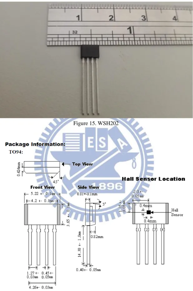
Hall Effect sensor we chosen is produced by Winson Semiconductor

Corporation. Its item number is WSH202, TO-94. Comparing with other continuous-time ratiometric linear Hall Effect Sensors, Hall Effect sensors produced by Winson have two advantages. First, it is the one of the continuous-time ratiometric linear Hall Effect sensors found with the most high operation frequency [20] [21] [22] [23] [24]. Second, according to the reference, these corporations, such as Melexis, Honeywell, ROHM, and Infineon, are foreign companies, but Winson is a company in Hsinchu, Taiwan. Hence, the symbols are easily obtained.

WSH202 integrates Hall sensing element, linear amplifier, sensitivity controller and emitter follower output stage. It accurately tracks extremely small change in magnetic flux density, which is generally too small to operate Hall Effect switch.

WSH202 can be applied as current sensor, tooth sensor, proximity detectors and motion detectors. As sensitive monitor of magnetic flux, it can effectively measure a system’s performance with negligible system loading while providing isolation from contaminated and electrically noisy environments

Followings are some details of the SPEC.

(35)

25

Figure 12. Equivalent circuit model and OUT vs Magnetic field [20]

Figure 13. Absolute maximum rating of WSH202 [20]

(36)

26

Figure 15. WSH202

(37)

27

3.1.3 Total system SPEC

In this section, whole system spec will be introduced. According to the Figure 4 and Figure.6, the transmitter equivalent model in coil system and the transmitter equivalent model in Hall Effect sensor system are the same. Using the same

transmitter provides the same condition to compare the performance of coil system and Hall Effect system. The following table shows parameters of the transmitter model.

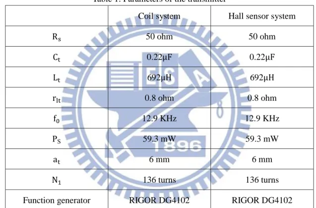
Table 1. Parameters of the transmitter

Coil system Hall sensor system

R_s 50 ohm 50 ohm Ct 0.22μF 0.22μF Lt 692μH 692μH r_lt 0.8 ohm 0.8 ohm f₀ 12.9 KHz 12.9 KHz PS 59.3 mW 59.3 mW at 6 mm 6 mm N₁ 136 turns 136 turns

Function generator RIGOR DG4102 RIGOR DG4102

R_s do not contain the output impedances of the function generators, which is 50 ohm, too. And R_s we chose here is cement wound resistors, which can endure more watt than the carbon film resistance. P_s is calculated by the equation (15) at f₀. Choosing resonate frequency at 12.9 KHz is to match the operation frequency region of the Hall Effect sensor.

(38)

28

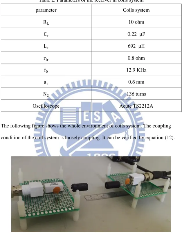
follows.

Table 2. Parameters of the receiver in coils system

parameter Coils system

R_L 10 ohm Cr 0.22 μF Lr 692 μH r_lr 0.8 ohm f₀ 12.9 KHz ar 0.6 mm N2 136 turns

Oscilloscope Acute TS2212A

The following figure shows the whole environment of coils system. The coupling condition of the coil system is loosely coupling. It can be verified by equation (12).

Figure 17. Coils system.

According to Figure.6, the spec of the receiver in Hall Effect sensor system is shown as follows.

(39)

29

Table 3. Parameters of the receiver in Hall Effect sensor systems

Parameter Hall sensor system

Rhall 332 ohm

DC bypass 14V

Magnetic sensitivity 10 mV/G

Operating current 3 mA

Maximum operation frequency 23 KHz

Oscilloscope Acute TS2212A

In the receiver of Hall Effect sensor system, resonate frequency of the transmitter must be lower than the maximum operation frequency of Hall Effect sensor. And due to the small operation current, the value of R_hall cannot be too small to induce voltages.

The following figure shows the whole environment of Hall Effect sensor system.

(40)

30

3.2 Steps of recording data

In this section, steps of recording data will be introduced. Methods of

experiments and recording data affect accuracy a lot. The reliable measurement data must have the strict steps. The following sections will show the steps of measuring data.

3.2.1 Steps of recording signals

Recording signals is a very important information in this study. Our goal is to measure the power transfer function at different frequencies. With the power transfer function at different frequencies and 3dB bandwidth, received power can be estimated more exactly.

(41)

31

Above figure shows the block diagram of recording signals. We record the signals by five steps. First step, set up whole system before we start to measure. Second step, adjust the distance between the transmitter and receiver from 1 cm to 3 cm. Each loop increase 0.5 cm. Third step, change the frequency of function generator from 5 KHz to 22 KHz, and record the measured signals at receiver. Operating

frequency of generator increases 1 KHz per loop. Fourth step, transform the recorded signals to frequency domain to obtain the peak voltage value at operating frequency. After the signals at whole conditions are recorded, power transfer functions at different frequencies and distances are acquired.

3.2.2 Steps of recording noise

Besides recording signals, noise is an important information in this study, too. In this system, Noise is mostly generated from two parts. First part is our measuring instrument, such as oscilloscope, and second part is our systems. We can distinguish these noises by measuring it at different settings.

(42)

32

The above figure shows the steps of recording noise is three scenarios. The first experimental scenario is measuring the noise of oscilloscope 𝑁₁. When oscilloscope is not connected with receiver, we can record the noise 𝑁₁ which oscilloscope shown to obtain the noise of measuring instrument.

In the second scenario, the noise of oscilloscope connected with the whole Hall Effect sensor system is 𝑁₁+ 𝑁_2hall. 𝑁_2hall is the noise in Hall Effect sensor system without function generator.

In the third scenario, the noise of oscilloscope connected with the whole coil system is 𝑁₁+ 𝑁_2coil. 𝑁_2coil is the noise in coil system without function generator. 𝑁_2coil is the noise in coils system without function generator.

After recording the data of the noise, transform the noise data to frequency domain and average the noise voltages in 3dB bandwidth per Hz to obtain the 𝑁₁, 𝑁2hall, and 𝑁2coil. According to the recorded noise, we can analysis what generates noise most.

3.2.3 Steps of calculating SNR, bandwidth and channel capacity

In this section, the steps of calculating the signal power and noise power will be introduced first. 3dB bandwidth will be introduced second. And the channel capacity will be derived in the end

df B P P B S L 



transfer funtion (35)

The received power we recorded is derived as above equation. The received power is multiplexed by the power transfer function and the transmitted power. The power transfer function is obtained by our measurement data at different frequencies

(43)

33

dividing transmitted power. And the transmitted power divides the 3dB bandwidth to know how many power are transmitted per Hz in 3dB bandwidth. And we sum up all the received power in 3dB bandwidth to get the exactly received power.

About noise, the unit of recorded data, such as 𝑁₁, 𝑁_2hall, and 𝑁_2coil, are mV per Hz. The noise power can be obtained by squaring 𝑁₁, 𝑁_2hall, and 𝑁_2coil, averaging the value in 3dB bandwidth, multiplexing bandwidth of coil system or Hall Effect sensor system , and dividing the resistor. The following equation shows the derivation of noise power.









coil L coil coil hall hall hall hall

B

R

N

E

N

B

R

N

E

N













]

)

(

[

]

)

(

[

2 2 1 2 2 1 (36) (37) Bandwidth in this study means 3dB bandwidth. 𝐵_hall represents the 3dB

bandwidth of Hall Effect sensor system. 𝐵_coil represents the 3dB bandwidth of Coil system. And the value of 3dB bandwidth can be acquired by the power transfer function recorded at section 4.1.

Channel capacity is the tightest upper bound on the rate of information that can be reliably transmitted over a communications channel. In this research, the

performances of Hall Effect sensor system and coil system are estimated by the channel capacity. With the measured data, the channel capacity can be derived as follows [11].

(44)

34





















system

sensor

Effect

Hall

,

system

coil

,

system

sensor

Effect

Hall

,

system

coil

,

log

10

₂ hall coil hall coil L

N

B

N

P

B

capacity

channel

(38)

(45)

35

Chapter 4 Results and discussion

In this chapter, the result of measurement and simulation will be shown.

Simulation result contains the received power calculated by equations in chapter 2 and PSPICE. Comparing the simulation result and the measurement result can assess advantages and disadvantages in Hall Effect sensor system and coil system more precisely. With the result of comparing, the performance of Hall Effect sensor system can be improved.

4.1 Power transfer function of coils and Hall sensor

system

In this section, the measuring data and the simulation result of energy transfer function in coil system and Hall Effect sensor system will be shown. The simulation result contains the current simulation of coil system in PSPICE and the equation of chapter 2. With the comparing the simulation result of PSPICE and the equation in chapter 2, it can verify the correctness of the equation (8).

(46)

36

Figure 21 shows coil system simulation model in PSPICE. The distance between Tx and Rx is 1 cm. The coupling coefficient can be derived by equation (3). The received current in receiver simulated by PSPICE is shown below.

Figure 22. Simulation of Received current in PSPICE

The simulation result is recorded to compare with the result calculated by equation (8). Following figure shows the comparing result.

Figure 23. Comparing result of equation (8) and PSPICE

Frequency 0Hz 2KHz 4KHz 6KHz 8KHz 10KHz 12KHz 14KHz 16KHz 18KHz 20KHz 22KHz 24KHz 26KHz -I(C2) 0A 4mA 8mA 12mA 16mA 20mA 24mA

(47)

37

From Figure 23. the received current derived from equation (3) has almost the same value as the current simulated by PSPICE, which means the equation (3) has been verified by the PSPICE.

Energy is derived from the current of receiver. The derivation of current has been proved. The next is the received power of coil system. 3dB bandwidth of the coil system can be measured from Figure 24.

Figure 24. Received power of coil system

Figure 24 shows the different power estimation of the coil system. Because the length of coil is closed to the transmission distance, the transmission distance must take the length of coil into consideration. It considers some situations, such as

effective distance is longer 10mm than the setup distance, effective distance is longer 4mm than the setup distance and the effective distance is the setup distance, to make the estimation more accuracy. However, the shape of the theory curve is still not

(48)

38

matched the measured data. The possible reason is that measured resonate frequency of measured data is deviated from the setup resonate frequency.

To measure the 3dB bandwidth more clearly, Figure 24 is zoomed in as

following figure. The measured 3dB bandwidth of coil system is about 4 KHz. And the measured power is close to the received power derived by equation (22). There is still a little inaccuracy between measured data and derivation result. But it is

acceptable, for its order of magnitude is smaller than 10dB.

Figure 25. Received power of coil system (zoom in)

The following figure shows the measured received power of Hall Effect sensor system and the power derived by equation (30).

(49)

39

Figure 26.Power transfer function of Hall Effect sensor system.

From figure.26 the measured power in Hall Effect sensor system is close to the received power derived by the equation (32). It proves our derivation of the received power in Hall Effect sensor system is accurate. And the 3dB bandwidth in Hall Effect sensor system is about 15 KHz.

In this section, we verify the measured power with the equation derived at chapter 2 and obtain the 3dB bandwidth both coil system and Hall sensor Effect system. In our experimental environment, the signal cannot be transmitted over 3 cm. Hence, the derivation of received power is important for researchers to estimate the system performance. With the 3dB bandwidth and the power transfer function obtained in this section, received power, signal to noise ratio and channel capacity of these two systems can be acquired.

(50)

40

4.2 Comparison of the signal to noise ratio (SNR) of

coils and Hall Effect sensor system

In this section, measured noise and power will be discussed. The signal to noise ratio will be shown, too. According to the acquired data, the difference between coil system and Hall Effect sensor system can be seen clearly. After the comparison between the noise and received power in coil system and Hall Effect sensor system, the improvability of Hall Effect sensor will be pointed out precisely, too.

The measured noise, N₁, 𝑁_{2ℎ𝑎𝑙𝑙} and N_2coil by the steps of Figure 20 is shown below.

Figure 27. The noise N₁ of oscilloscope.

Figure.27 shows the measured noise of oscilloscope. In the experiment environment, some noise belong to the measuring instrument rather than the receiver

(51)

41

system. To get the more precisely comparison, the noise of the measuring instrument N₁ must be recorded first to distinguish the noise between receiver system and the whole system including the oscilloscope. The averaged value in 5 KHz to 22 KHz of the squared noise 𝑁₁2_is_{2.88 × 10}−11_𝑉2_/𝐻𝑧

Figure 28. The noise of the oscilloscope and Hall Effect sensor system

Figure 28 shows the noise of the oscilloscope cascading Hall Effect sensor system. The averaged value in 5 KHz to 22 KHz of the squared noise N₁+N_2hall is 2.285 × 10−8_𝑉2_/𝐻𝑧.

(52)

42

Figure 29. The noise of the oscilloscope and coil system

Figure 29 shows the measured noise of the oscilloscope cascading coil system. The averaged value in 5 KHz to 22 KHz of the squared noise is 2.91 × 10−11𝑉2

To conclude the result of the noise measurement, it is obvious that the oscilloscope cascading Hall Effect sensor system generates more noise than the oscilloscope cascading coil system. According to the measurement result, 𝑁₁+ 𝑁_{2𝑐𝑜𝑖𝑙} and 𝑁₁ have the same order of magnitude. The value of 𝑁_2coil compared with 𝑁₁ is very small, so that the impact of 𝑁_2coil can be ignored in the coil system. The processes behind the receiver in the coil system affect the noise level most.

However, the receiver noise in Hall Effect sensor system dominates the system performance. According to the recorded data, 𝑁₁+ 𝑁_2hall is 1.33 × 10−4 V. But 𝑁1 is only 4.75 × 10−6 𝑉. The gap of order of magnitude between 𝑁2hall and 𝑁1 is 2. In Hall Effect sensor system, the noise generated from the Hall Effect sensor dominates the whole system.

(53)

43

Received signal power is calculated by the equation

(35) with the power transfer function at section 4.1. Besides the recorded signal power, the derivation of received power in the coil system by equation (24), and the derivation of received power in Hall Effect sensor system by equation (32). The figure of comparing the received power in theory and recorded data is shown below.

Figure 30. Power received versus distance

From Figure 30 the value of theory power and measured power are closed. Due to the limited of experimental apparatus, the signal can be received and detected at most 3 cm. To see the limit of the performance, the estimation of received power is shown. Both the coil system and Hall Effect sensor system decay 40 dBm at 10 cm. The received power of coil system is about 37dBm higher than the received power of Hall Effect sensor system. It shows the room for improvement of Hall Effect sensor system. The inaccuracy of measured coil power is mainly due to the inaccurate distance

(54)

44

between the transmitter and the receiver. From the recorded data, the smaller setup distance is, the larger error it will be. This error is come from that the effective distance is larger than the setup distance.

3 3 2 2 3 2 2 eff 3 3 2 2 3 2 2 3 2 2 3 2 ) )( ) ) (( 1 ) ( 1 ( into repalced be can power received the of error to l propotiona is ch factor whi the is ) )( ) ( 1 ) ( 1 ( ) ( ) ( t coefficien coupling squared the to l propotiona is power received and the between error the is r t t set t set set r t t eff t set t r t L set eff set eff set eff a a a c d a d c d d a a a d a d a d a a k P d d c c d d d d                    (39)

From equation (39), it shows why the smaller setup distance is, the larger error it will be.

Besides, the coil received power takes the advantage at the measured data. Because the coil we choose can sense more magnetic fields than the Hall Effect sensor by its longer radius and the magnetic materials in the center of coil. The longer radius makes it have more area to sense the magnetic flux. And the magnetic materials in the center of coil can enhance the magnetic flux, too .The gap of received power between the coil system and Hall Effect sensor system should not be large as

providing data. The following figure shows the simulation of the coil, which has the same area to sense the magnetic flux as Hall Effect sensor.

Figure 30 also shows the gap between the coil system and the Hall Effect sensor system is reduced to 20 dB. If the coil we chosen has the same area to sense the magnetic flux as Hall Effect sensor, the gap between Hall Effect sensor and the coil system will be closer than the gap of the data we measured.

霍爾感應器用於近場磁感應通訊之探討

國立交通大學

電子工程學系電子研究所碩士班

碩士論文