適用於分散式存取系統且具有強健性的劃分演算法

i

國

立 交 通 大 學

電信工程學系

碩 士 論 文

適用於分散式存取系統且具有強健性的劃分演

算法

A robust splitting algorithm for the

distributed access system

研究生：柯富元

指導教授：廖維國 博士

適用於分散式存取系統且具有強健性的劃分演算法

A robust splitting algorithm for the distributed

access system

研 究 生︰ 柯富元

Student: Fu-Yuan Ko

指導教授︰ 廖維國 博士

Advisor: Dr. Wei-Kuo Liao

國 立 交 通 大 學

電信工程學系碩士班

碩士論文

A Thesis Submitted to

the Department of Communication Engineering

College of Electrical and Computer Engineering

National Chiao Tung University

in Partial Fulfillment of the Requirements

for the Degree of Master of Science

In

Communication Engineering

July 2008

Hsinchu, Taiwan, Republic of China

適用於分散式存取系統且具有強健性的劃分演算法

研 究 生︰ 柯富元

指導教授︰ 廖維國 博士

國立交通大學電信工程學系碩士班

中文摘要

在無線通訊上,分散式媒介允許控制(Medium Access Control)協訂常用於傳送資料。 我們考量輸出以及當錯誤發生時的穩定性來設計我們的協定為了解決輸出過低的問 題，我們參考兩種不同的媒介允許控制協定,slotted Aloha 和劃分演算法(Splitting algorithm)為了改善這兩者的缺點我們提出一種輸出和劃分樹狀演算法的輸出差不多且 在對抗錯誤傳輸時更強健的協定。和劃分樹狀演算法不同得是我們的協定更適用於較分 散式的系統。由於在我們的協定中我們假設每個使用者都知道現在有多個使用者想要傳 送所以我們稱呼我們的協定為 N 以知的劃分演算法。這個方法的輸出約 0.45。而強健 在無線通訊上另一個重要問題。此外我們針對錯誤傳輸列舉了一些極端的情形並且去討 論我們的方法對錯誤傳輸的容忍度。並且模擬在不同的錯誤率下的輸出。根據模擬結果 我們可得知在錯誤率很小的情形我們的輸出約等於無錯誤時的輸出減去錯誤率。

A robust splitting algorithm for the distributed

access system

tStudent: Fu-Yuan Ko Advisor: Dr. Wei-Kuo Liao

Department of Communication Engineering

National Chiao Tung University

Abstract

Distributed MAC protocols have long been used in the existing wireless communications for data transfer. In devising our protocol, both throughput and robustness against error-prone transmission are considered. In order to improve the throughput, our proposed protocol is based on two kinds of medium access control protocol, Slotted Aloha and splitting algorithm. In doing so, our proposed protocol supplements the drawbacks of these two protocols by achieving the throughput as high as the splitting tree algorithm whereas sustaining the robustness against the error-prone transmission. Besides, unlike the splitting tree algorithm, our protocol can be rendered into the highly distributed system. Due to the assumption that the number of active or so-called backlogged users needs to be known in our protocol a priori, we call it as “N is known splitting algorithm”. By analysis, we show that the maximum throughput of our proposed protocol is around 0.45. In addition, we enumerate certain critical cases and discuss the capability of our method against the erroneous transmission. We simulate our method in different error rate and verify their throughputs. According to our simulation results, we can find that our throughput of an error rate is similar to the throughput of no error minus the error rate when the error rate is small enough.

誌謝

首先，感謝指導教授廖維國老師，在研究所的三年時光，老師都給予我許多的 指導 ; 也感謝交通大學的張文鐘老師，以及田伯隆老師，能夠在百忙之中抽空前來參加 口試，並給予我論文上的指導與建議。 終於完成一篇屬於自己的論文，我內心的雀躍真是筆墨無法形容的 ; 回顧這三 年的研究所生涯， 不論是期末考的挑燈苦讀、還是跟實驗室的大家一起歡唱 KTV …， 都是我的美好回憶。此時此刻，我的內心真可說是百感交集，一方面正期待完成碩士學 業的未來生活，另一方面也對即將離開交通大學感到不捨。 尤其是充滿歡樂的 812b 實 驗室，大家給予我這溫暖的友情，是我一輩子也不會忘記的 ; 學長黑熊還有毛毛、為凡、 賢宗及柔嫚、國瑋學姐在我研究遇到瓶頸時，主動提供我相關的資訊，適時點醒我心中 的盲點 ; MOON、陳俊宏、是我研究所同甘共苦的好夥伴，一起討論課業，一起打屁嬉 鬧 。 從小到大，媽媽在我遭遇挫折的時候，總是給我鼓勵，教導我相信自己，相信 一定能突破困難，使我學會樂觀的看待生活中的不順遂 。祖母也會常常幫我祈禱,使我 在這幾年雖然有些小意外但也都平安的度過了。 謝謝大家。

Contents

Chinese Abstract………...……….iii English Abstract……….……….iv Acknowledgement………...v Contents……….………...vi List of Figures……….……….………vii Chapter 1: Introduction………….………..1

Chapter 2: Background knowledge………...………3

2.1 Slotted Aloha……….………….…….……….3

2.2 Tree splitting algorithm……….5

2.3 FCFS splitting algorithm……….…….………7

2.4 Tree algorithm using successive interference cancellation………...9

Chapter 3: N is known splitting algorithm………...10

3.1 Model.……….……..………...………...10

3.2 N is known splitting algorithm………….…..………11

3.3 N is known splitting algorithm in distributed system ………...……….13

Chapter 4: Analysis……….15

4.1 Throughput analysis………...15

4.2 The node behavior when an error occurs………18

4.2.1 Idle detected to collision………..19

4.2.2 Collision detected to idle……….20

4.2.3 Success detected to collision……….21

4.2.4 Success detected to idle………..21

Chapter 5: Simulator Design…….……….23

Chapter 6: Simulation Results………...………..………25

Chapter 7: Conclusion………...28

List of Figures

Number Page

2.1 Slotted Aloha Success (S) Collision(C) Empty (E)……….3

2.2 Departure rate as a function of attempted transmission rate G for slotted Aloha [2]………...4

2.3 An example of tree algorithm………...5

2.4 FCFS splitting algorithm improvement 1 [2]………7

2.5 FCFS splitting algorithm improvement 2 [2]………8

3.1 Cases of the end of a CRP. The yellow subset is the end of a CRP and the number in a subset is the number of nodes in this subset………..11

3.2 The example of N is known splitting algorithm………..12

4.1 Some cases of splitting when k=2………...16

4.2 The example of “collision detected to idle”………20

4.3 The example of “success detected to collision………21

4.4 The example of “success detected to idle”………...22

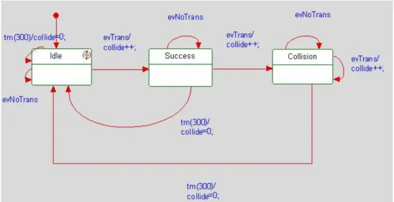
5.1 UML state-chart for Node………...23

5.2 UML state-chart for Channel………..24

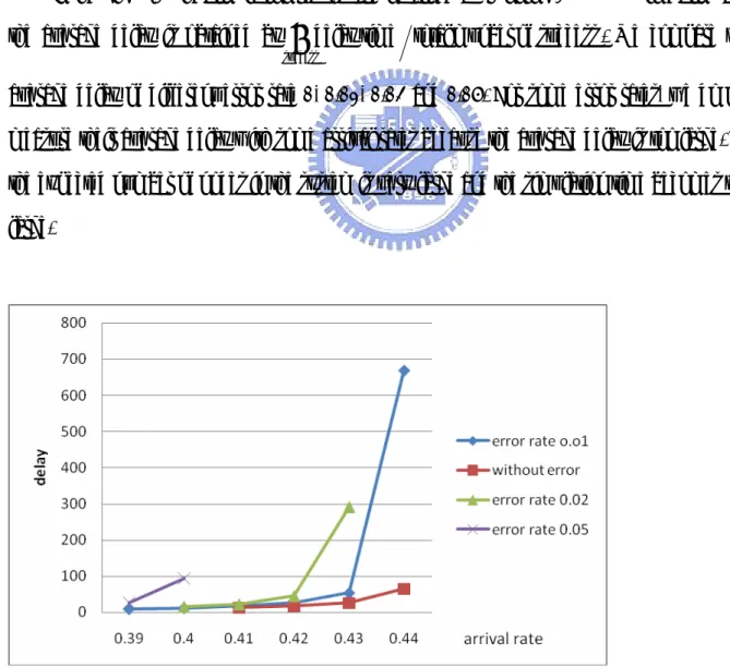
6.1 The average delay vs. arrival rate of different error rate………....25

6.2 Throughput vs. arrival rate of different packet error rate with running time 10,000 time slots………26

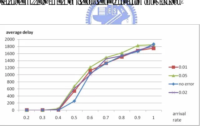
6.3 Average delay vs. arrival rate of different packet error rate with running time 10,000 time slots………27

Chapter 1

Introduction

Distributed MAC protocols have long been used in the existing wireless communications for data transfer. Essentially with such a protocol in place, a user participating in the wireless communication may send its packet at the beginning of a time slot and wait for the positive acknowledgment. There are three possible outcomes immediately after a time slot: First, only single packet is transmitted in the time slot and a positive acknowledgment is detected by all users. Such a situation stands for a successful transmission, denoted by “1”. Second, if there is no data being sent, all users will detect an idle status during the time slot, denoted by “0”. Finally, two more packets being sent will mark a collision because there is no positive acknowledgment received, denoted as “e”.

To enhance the throughput of the distributed MAC protocol, there are two major classes of algorithms having been proposed, namely the Slotted Aloha and tree splitting algorithm. The basic operation of Slotted Aloha is assuming that each user knows the number of users being requested to send their packets, so called backlogged users. Based on such a number, say N, the user then send its packet with the transmission probability as 1/N. In [1][2], the analysis has shown that such a way to set its transmission probability is optimal and the throughput is at most 1/e if the arrival of backlogged users follows the identical Poisson distribution.

Tree Splitting algorithm is an approach that divides the users involved in a collision into several subsets using some tree like mechanism [2][3]. Only the users or users in one of the subsets will transmit at the next time so the probability of collision is reduced. The maximum throughput in the splitting algorithm is about 0.43 [3]. Though it performs better than Slotted Aloha, however it needs a common receiver to achieve its algorithm.

In the splitting algorithm, the common receiver plays a very important role. It need send the feedback to each node, block the new nodes which arrive in the collision resolution period (CRP) [2] and split the new nodes into a correct number of subsets.

In our research, we consider a new distributed MAC algorithm that does not use the common receiver, which is necessary in Splitting-Tree Algorithm, but each node has the information of N, as in Slotted Aloha. We call this new algorithm as “N is known splitting algorithm”. Because of no common receiver, each node need detect the channel state instead of the feedback and judges the CRP by itself. Besides, the “N is known splitting algorithm” do

some changes, and its throughput can is about 0.45. We assume that the channel is a “Noisy collision channel” [4]. Each node might detect the wrong channel state because of the noise. The robust issue is very important to the tree splitting algorithm. For example, if an idle slot is incorrectly perceived by the common receiver as a collision, all nodes will not transmit in the next two slots. So we discuss the robust issue in our method and discuss the behavior of the error nodes.

The rest of the thesis is organized as follows. In chapter 2 we introduce the background knowledge of our study. The system framework is presented in chapter 3. And the analysis of “N is known splitting algorithm” is described in chapter 4. The design in our simulator is illustrated with simulator graphs in chapter 5. Simulation results are reported in chapter 6, followed by conclusion in chapter 7.

Chapter 2

Background knowledge

In this chapter we will introduce the basic concept of Slotted Aloha and Tree Splitting Algorithm.

2.1 Slotted Aloha

In the slotted Aloha, we assume that all transmitted packets have the same length and each packet requires one time unit (call a slot) for transmission. All transmitters are synchronized and each node transmits in the beginning of a slot. If a new packet arrives in a slot, it will not transmit until the beginning of next slot.

When a collision occurs in slotted Aloha, each node sending one of the colliding packets discovers the collision at the end of the slot and become backlogged. If each backlogged node were simply retransmit in the next slot after being involved in a collision, then another collision would surely occur. Each node retransmit packet with probability p when a collision occurs. We give an example in Fig. 2.1. In Fig. 2.1, three nodes collide at the slot 1 so they retransmit packet with probability p until they retransmit successfully.

Figure 2.1 Slotted Aloha Success (S) Collision(C) Empty (E)

We assume that the arrival rat in one slot is λ. Define the attempt rate G(n) as the expected number of attempted transmissions in a slot when n backlogged in the system.

G(n)=λ+np (2.1) If p is small, P is closely approximated as the following function of the attempt rate: _succ

( )

) ( G n succ G n e

P ≈ − (2.2) This approximation is derived directly from Eq. (2.2), using the approximation (1-x)y ≈ e - xy

for small x. This relationship is illustrated in Fig. 2.2. Similarly, the probability of idle slot is approximately e–G(n).

Fig 2.2 Departure rate as a function of attempted transmission rate G for slotted Aloha [2]

2.2 Splitting Tree Algorithms

The slotted Aloha requires some care for stabilization and is also essentially limited to throughputs of 1/e. We now want to look at more sophisticated collision resolution techniques that both maintain stability and also increase the achievable throughput. A splitting algorithm is an approach that divides the users involved in a collision into several subsets. Only the user or users in one of the subsets will transmit at the next time slot so that the probability of collision is reduced.

The first splitting algorithms were algorithms with a tree structure. When a collision occurs, say in the kth slot, all nodes not involved in the collision go into a waiting mode, and all those involved in the collision split into two subsets (e.g., by each flipping a coin). The first subset transmits in slot k+1, and if that slot is idle or successful, the second subset transmits in slot k+2 (see Fig. 2.2). Alternatively, if another collision occurs in slot k+1, the first of these two subsets split again, and the second subset waits for the resolution of that collision.

Figure 2.3An example of the tree algorithm

The rooted binary tree in Fig. 2.2 represents a particular pattern of idles, success, and collision resulting from such a sequence of splitting. S represents the set of packets in the original collision, and L (left) and R (right) represent the two subsets that S splits into. Similarly, LL and LR represent the two subsets that L splits into after L generates a collision. The set of packets corresponding to the root vertex S is transmitted first, and after the transmission of the subset corresponding to any nonleaf vertex, the subset corresponding to the vertex on the left branch, and all of its descendant subsets, are transmitted before the subset of the right branch. Given the immediate feedback we have assumed, it should be clear

that each node, in principle, can construct this tree as the 0, 1, e feedback occurs; each node can keep track of its own subset in the tree, and thus each node can transmits its own backlogged packet.

The transmission order above corresponds to that of a stack. When a collision occurs, the subset involved in collision is split, and each resulting stack is pushed on the stack (i.e., each stack element is a subset of nodes); then the head of the stack (i.e., most recent subset pushed on the stack) is removed from the stack and transmitted. The list, from left to right, of waiting subsets in Fig. 1 corresponds to the stack elements starting at the head for the given slot. Note that a node with backlogged packet can keep track of when to transmit by a counter determining the position of the packet’s current subset on the stack. When the packet is involve in a collision, the counter is set to 0 or 1, corresponding to which subset the packet is placed in. When the counter is 0, the packet is transmitted, and if the counter is nonzero, it is incremented by 1 for each collision and decremented by 1 for each success or idle.

One problem with this tree algorithm is what to do with the new packet arrivals that come in while a collision is being resolved. A collision resolution period (CRP) is defined to be completed when a success or idle occurs and there are no remaining elements on the stack (i.e., at the end of slot 9 in Fig. 1). At this time, a new CRP starts using the packets that arrived during the previous CRP. In the unlikely event that a great many slots are required in the previous CRP, there will be many new waiting arrivals, and these will collide and continue to collide until the subsets get small enough in the new CRP. The solution to this problem is as follow: At the end of a CRP, the set of nodes with new arrivals is immediately split into j subsets, where j is chosen so that the expected number of packets per subset is slightly greater than 1 (slightly greater because of the temporary high throughput available after a collision). These new subsets are then placed on the stack and the new CRP starts.

2.3 FCFS Splitting Algorithms

Another famous splitting algorithm is first-come-first-serve (FCFS) splitting algorithm. It splits the colliding packets into two subsets by packet arrival time and it always transmits the earlier arriving first. This algorithm can achieve the maximum throughput 0.4871 [2]. In this algorithm, the common receiver sends an “Allocation interval” to each node and only the nodes which have packets arriving in this “Allocation interval” can transmit. We denote it as S. If a collision occurs, the common receiver sends a new “Allocation interval” to each node, this new allocation interval is only half of S but their starting points are the same. We denote this new interval as L and the other interval as R. It seems very similar with tree splitting algorithm, but its throughput is higher. We illustrate the improvements in Fig.2.4 and Fig.2.5.

In the Fig.2.4, we assume the allocation interval for slot k is from T(k) to T(k)+α(k). When a “Collision” occurs in slot k, the allocation interval is split into two equal subintervals and the leftmost subinterval L is the allocation interval in slot k+1. Thus, T(k+1) = T(k) andα(k+1) =α(k)/2. When an “Idle”, as in slot k+1, follows a collision, one improvement to the tree splitting algorithm is employed. The previous rightmost interval R is known to contain two or more packets and immediately split, with RL forming the allocation interval for slot k+2. Thus, T(k+2) = T(k+1)+α(k+1) andα(k+2) =α(k+1)/2. Finally, successful transmissions occur in slot k+2 and k+3, completing the CRP.

another improvement to tree algorithm is employed. Since interval L contain two or more packets, the “Collision” in slot k tell us nothing about interval R and we would like to regard R as if it had never been part of an allocation interval. As shown for slot k+2, this simplicity itself. The interval L is split, with LL forming the next allocation interval and LR waiting; the algorithm simply forgets R. When LL and LR are successfully transmitted in slot k+2 and k+3, the CRP is end.

However, this algorithm needs the common receiver for sending the allocation time, and it needs many times to split the colliding interval into a very small subinterval to resolve the colliding packets whose arrival intervals are very close. Besides, the first improvement has a slight problem in the robust issue. If an idle slot is incorrectly perceived by the common receiver as a collision the algorithm continuous splitting indefinitely, never making further successful transmission. So we don’t use this algorithm in our research, but we refer its improvement method and do some changes in our research.

2.4 Tree algorithm using successive interference cancellation

In this method [5], its throughput can achieve 0.693. The main ideal of this method is

that we can get some information even the collision occurs. We assume that two nodes, A and B, transmit their packets to the receiver. So the received vector is: y1=A +B+ n, where n denote a noise vector. If only A sends its packet in the next slot, the received vector is: y2=A +nA. At the end of this slot, packet A is decoded and then cancelled to obtainy1 =xB +nA +n

~

. If n_A+ is sufficiently small, we can decode B in the same slot. So we use two slots and n

transmit two packets even when the collision occurs in first slot.

However, we do not use this method in our research, because it needs a complex receiver and we don’t see any product using this method. Besides, this method can’t use in distributed system.

Chapter 3

N is Known Splitting Algorithm

In this chapter we will introduce the hybrid splitting algorithm, in the algorithm we assume that the numbers of nodes, N, which have backlogged packets are known by each node. So we name this splitting algorithm as “N is known splitting algorithm”.

3.1 Model

We list the assumptions of the model and then discuss their implications.

1. Slotted system. Assume that all transmitted packet have the same length and that each packet requires one time unit (call a slot) for transmission. All transmitters are synchronized so that the reception of each packet starts at an integer time and ends before the next integer time.

2. Poisson arrivals. Assume that packets arrival for transmission at each of the m transmitting nodes according to independent Poisson process. Let λ be the overall arrival rate to the system,

3. Noisy collision channel. Assume that if two or more nodes send a packet in a given time slot, then there is a collision and receiver obtain no information about the contents or source of the transmitted packet. But packets can be corrupted also by noise even when collisions are absent.

4. 0,1,e Immediate feedback. At the end of each slot, each node detects whether 0 packet, 1 packet or more than one packet were transmitted in that slot.

5. Retransmission of collisions. Assume that each packet involved in a collision must be retransmitted in some later slot, with further such retransmission until the packet

be backlogged.

6. A .No buffering. If one packet at a node is currently waiting for transmission or colliding with another packet during the transmission, new arrivals at that node are discarded and never transmitted. An alternative to this assumption is the following.

B. Infinite set of nodes (m=∞). The system has an infinite set of nodes and each

newly arriving packet arrives at a new node.

3.2 N is known splitting algorithm

In the “N is known splitting algorithm”, we have some differences with the “tree splitting algorithm”.

1. In the CRP start each node transmits with probability 1/N. So we might transmit successfully in one slot with probability 1/e, when N is large enough.

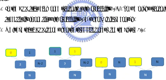
2. We judge that a CRP is end when the three cases occur, see the Figure 3.1.

Figure 3.1 Cases of the end of a CRP. The yellow subset is the end of a CRP and the number in a subset is the nodes in this subset.

2.1 The “Idle” occurs. We assume that a collision occurs in the subset L in the slot k. So we know that there are more than or equal to 2 nodes in the subset L. Then the nodes in subset L must split into two small subsets, LL and LR. If the LL subset transmit and an “Idle” occurs in the slot k+1, we know that there is no node in the subset LL and there are more than or equal to 2 nodes in the subset

LR. So we should not transmit the subset LR in the slot k+2.

2.2 Two continuous “Success” occur. Because this case must happen in the end of a branch and we do not know how many nodes are in the other branch.

2.3 An “Idle” or a “Success” occurs in the slot of the “CRP start”.

3. We add a flag to support 2.2 and 2.3. The flag is a local variable for each node and is set as 1 when a CRP starts. This flag will increase 1 if a “Success” occurs and will be set as 0 if a “Collision” occurs. So we can judge that the CRP is end when an “Idle” occurs or the flag is 2.

Similar to the tree algorithm, a node with a backlogged packet can keep track of when to transmit by its counter (e.g., when the counter is 0, the packet is transmitted). The initial value of the counter is 0, and this value will be changed according to the following statement.

If this node is split into the subset L when the CRP starts, its counter is set to zero. Alternatively, if this node is split into the subset R when the CRP starts, its counter is set to a large number (e.g., 1000). During the CRP, if the counter is not zero, it is increased by 1 for each collision and decremented by 1 for each success. If the counter is zero, it is set to 0 or 1, corresponding to which subset the packet is placed in when a collision occurs, and it is set to 0 when a success or idle occurs. When the CRP is completed, the counter will be initialized to 0. According to these descriptions, we give an example in Figure 3.2.

In the Fig 3.2, we assume that N nodes want to transmit when a CRP start, these nodes split into subset L and subset R with probability 1/N and N-1/N, respectively. The nodes of subset L transmit in slot 1, and the nodes of subset R wait in slot 1. Because the feedback in slot 1 is “Collision”, the subset L splits into two subsets (LL and LR) with equal probability. The nodes of the subset LL transmit in slot 2 and the nodes of subset LR and subset R wait in slot 2. Unfortunately, the feedback in the slot 2 is “Collision”, so the subset LL split into two small subsets (LLL and LLR). Then the nodes of subset LLL transmit in slot 3 and the nodes of subsets R, LR and LLR wait in the slot 3. Fortunately, the feedback in the slot 3 is “Success”. Then the nodes of LLR transmit in the slot 4 and the nodes of subsets R and LR wait. Because the feedback in slot 4 is also “Success”, we end this CRP.

3.3 N is known splitting algorithm in the distributed system

When we apply the “N is known splitting algorithm” in the distributed system, we have some problem about the immediate feedback. We will discuss these problems and modify the algorithm.

3.3.1 Detection rules

In the distributed system, each node senses the channel by itself and the immediate feedback will not be send by the common receiver. Each node detects the channel states in each time slot to instead the immediate feedback. Like the common receiver, we assume that each node can detect three kinds of channel states, “Idle”, “Success” and “Collision”. We define some detection rules that help each node to detect the channel.

1. The channel state is “Idle” if the node detects the SNR is below the threshold.

2. The channel state is “Collision” if the node detects the SNR that is over the threshold. 3. The received node must broadcast ACK to each node if it receives a packet and the CRC

is correct.

4. The transmitter can’t sense the channel when it transmits. So if the transmitter doesn’t receive the ACK, it judges that the channel state is collision.

5. Each node judges that the channel state is success when it receives the ACK.

Chapter 4

Analysis

In this section, we will analyze the average throughput and the behavior when the error occurs in the system that use the N is known splitting algorithm. We analyze the throughput without error and find the maxima stable throughput in section 4.1. Then we discuss all case of error and analysis the effect for each case in section 4.2.

4.1 Throughput analysis

The average throughput is equal to the total successful number divided by the total time slots. In N is known splitting algorithm, we divide the total time slots into several CRPs so the expected value of the throughput in a CRP is equal to the average throughput.

(4.1) CRP] a in slots time E[ CRP] a in numbers successful E[ CRP] a in ut E[throughp Throughput Average = =

To calculate the equation we need to calculate attributes first.

Tk: the expected value of time slots in a CRP given the condition that k nodes split to the left subset when a CRP starts.

Sk: the expected value of successful nodes in a CRP given the condition that k nodes split to the left subset when a CRP starts.

Pk: the probability that k nodes split to the left subset when a CRP starts. So the equation (4.1) may be restated as

(4.2)

∑

∑

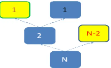
= k k k k k k T P S P Throughput

To find Tk we need to find T0, T1, T2 …Tk-1. It is very easy to find thatT₀ =1,T₁=1, but T2 is not easy to find. Because two nodes transmit in the same time slot, collision must happen. The two nodes must split again, and the probability that j nodes will be split in the left subset in the second layer is 2 ₎2

2 1 (

j

C , see the Fig.4.1.

Fig.4.1 some cases of splitting when k=2

If j= 0, according to the algorithm we descript in the chapter 3, this CRP will end and the length of CRP is equal to 2. If j=1, this node transmit and the other node will transmit in the next time slot then the CRP will end. So the length of CRP is equal to 3. If j=2, see the right illustration in Fig.4.1,the two node will split again and the behavior is like the left illustration in Fig.4.1.So )] 3 ( ) 2 1 ( ) 2 ( ) 2 1 ( [ ] ) 2 1 ( [ 2 2 1 2 2 0 0 2 2 2 C C i C i T i i + + + =

∑

∞ = (4.3)

3 T as follow (4.4) )] 1 ( ) 2 1 ( [ )] 2 ( ) 2 1 ( [ )] 2 ( ) 2 1 ( [ ) 2 1 ( 3 3 ₂ 2 2 3 3 1 3 3 0 3 0 3 3 3 =

∑

+ + + + + + + ∞ = T i C T i C i C C T i i

where i is the frequency that three nodes are split in the left subset. According to the equation (4.4), we can find that

(4.5) 2 k for ) 2 ( ) 2 1 ( ) 1 ( ) 2 1 ( 2 1 T 1 _{1 1} 1 ; 0 0 k ≥ ⎪⎭ ⎪ ⎬ ⎫ ⎪⎩ ⎪ ⎨ ⎧ + + × × + ⎥ ⎦ ⎤ ⎢ ⎣ ⎡ + + × × ⎟ ⎠ ⎞ ⎜ ⎝ ⎛ = − ₋ ≠ = ∞ =

∑

∑

k k k k j j j k k j ki i T i C T i C

where i is the frequency that k nodes are split in the left subset.

We use a similar way to calculate Sk by S0, S1, S2,…,Sk-1. Obviously, S0 is equal to 0 because no node transmits in the CRP and S1 is equal to 1 because only one node transmits in the CRP. We assume that there are j nodes split in the left subset where0≤ j≤2. If j is equal to 0, no nodes will be transmitted and the CRP will end. If j is equal to 1, the node of left subset is transmitted successfully. The node of right subset will be transmitted successfully in the next time slot then the CRP will end. If j is equal to 2, the two nodes must collide and are split again until 0 or 1 node split in the left subset.

(4.6) ) 1 ( ) 2 1 ( ) 2 1 ( 2 2 ₁ 1 0 2 2 =

∑

× + ∞ = S C S i i

(4.7) } ) 1 ( ) 2 1 ( ] ) 2 1 ( {[ ) 2 1 ( 1 2 1 1 0

∑

∑

− = − ∞ = + × × + × × = k j k k k j k k j i ki k C S C S S

where i is the times that k nodes are split in the left side and j is the number of nodes that are split in the left side.

Because each nodes may transmit with probability 1/N when a CRP starts, the probability that k nodes are divided in the left subset,P_k, is equal to N k N k

k

N N N

C ₍1_{) (} −1₎ − _{. In}

order to find the stable average throughput, we assume thatN→∞, then

(4.8) ! 1 ) 1 ( ) 1 ( lim e k N N N C P N k N k k N k ≅ _× − = − ∞ →

According to the equation (4.2), (4.5), (4.7) and (4.8) we can find the average throughput and its value is approximate to 0.45 packets per time slot.

4.2 The node behavior when error occurs

In the true environment, the packets transmit in the noisy collision channel. Unlike the noiseless collision channel model packets can be corrupted also by noise even when collisions are absent. In the noisy collision channel, even if only one node transmits during a time slot, its packet can still be corrupted by noise. Suppose that binary phase shift keying (BPSK) is used to modulate the information bits per packet, and let ρ =E_b / N₀ denote the signal-to-noise ratio (SNR) per bit, where E_band N₀ are the bit energy and one-side noise power density, respectively. For the additive white Gaussian noise (AWGN) channel, the bit error rate is given by P =Q( 2E /N ) , where Q x e y2/2dy

) 2 / 1 ( : ) ( =

∫

∞ π − is the

Marcum’s Q-function. Moreover, we assume that a packet comprising L_p bits can be successfully recovered only if all its bits are correctly received. The corresponding packet error rate (PER) is then given by Lp

b

e P

P =1−(1− ) _.

There are four detective errors in my simulation. First, idle detected to collision. It happens when no nodes transmit but the noise around the error nodes is too large such that the nodes detect error. Second, collision detected to idle. It happens when the node detects the signal intensity bellowing the threshold, but there are more than two nodes send packets. Third, success detected to idle. It happens when the node detects the signal intensity bellowing the threshold, but only one node transmits in the system. Fourth, success detected to collision. It happens when the node detects the signal intensity over the threshold, but only one node transmits in the system. We do not discuss with two cases, idle detected to success and collision detected to success, because their probability is too low.

4.2.1 Idle detected to collision

A node might detect the collision when no one transmits, if the noise around it is too large. In the N is known splitting algorithm, this node will increase its counter by 1. So its counter is more than or equal to 2. The other nodes will enter a new CRP because they detect the collision. This error node can’t transmit in the new CRP because its counter can’t decrease to 0 before the end of this CRP.

To analyze the effect of this case, we assume that a node has this error. We discuss the change of idle, success and collision probability in the next time slot and assume that no error occurs and no new packet arrives in the next time slot for the convenience.

The probability of “Idle” will become ₍ −1₎N−1

N N

and this value is more than N

N N

) 1 ( − , the idle probability without error. The successful probability will become ₍ −1₎N−1

N N

and this value is the same as₍ −1₎N−1

N N

, the successful probability without error. The probability of “Collision” will decrease because the summation of the three probabilities is 1.

4.2.2 Collision detected to idle

A collision slot is incorrectly perceived by a node as an idle if its signal intensity is below the threshold. In this case, the error node judges that the CRP ends because it perceives the channel as an idle and it will transmit with probability 1/N in the next slot.

In this case, the expected value of the transmitter in the next slot will increase. Because the error node would not transmit in the next slot if the error doesn’t occur.

To analyze the effect of this case we give an example in Figure 4.2. We assume that the error occurs in the second slot of the CRP and the error node is in the “N-3” subset. So the probability of collision in the third slot is ) (1)

2 1 ( ) 4 1 ( N ×

+ , the probability of success in the third slot is )(1) 4 1 ( ) 1 )( 2 1 ( N N N− ₊

and the idle probability in the third slot is )( 1) 4 1 ( N N− . Compare this probability with the non-error case, the probability of collision in the third slot is increase 1/2N and the probability of success and idle decrease 1/4N respectively. We can ignore these differences when N is large.

4.2.3 Success detected to collision

A successful slot is incorrectly perceived by a node as a collision if the receiver doesn’t

receive the packet successfully and this node perceives incorrectly because of the noise. We will discuss the effect in this case with the error nodes that transmit or not. The transmitter must be an error node in this case, so it will flip a coin to decide transmitting or not in the next slot. If a node that doesn’t transmit in this time slot occurs this error, it will add its counter and will not transmit in the next slot.

To analyze the effect of this case, we assume that the transmitter and one node of the subset R have this error. Obviously, the throughput must decrease in this case because packet should transmit successfully if error doesn’t occur.

We give an example in Fig 4.3. If error doesn’t occur, we spend three slots and have two successful transmissions in the CRP. If error occurs at the second slot of the CRP and if the transmitter in this slot decides to transmit in the third slot, the collision must occur in the third slot. Unfortunately, if no one can transmit in the fourth slot after splitting, the CRP ends and we spend four slots and have no success in the CRP. We do not discuss the error node of the subset R because it can’t transmit in this CRP.

Fig. 4.3 the example of “success detected to collision”

4.2.4 Success detected to Idle

receive the packet successfully and this node perceives incorrectly because of the noise. We will discuss the effect in this case with the error nodes that transmit or not. This error would not occur in the transmitter because the transmitter perceives the channel as a collision when it doesn’t receive the ACK. So we discuss this case for the nodes that doesn’t transmit.

We assume that a node that doesn’t transmit has this error and the transmitter detect the “Success” as the “Collision”. We give an example in Fig 4.4. Similar to the example in Fig 4.3, we assume that error occurs at the second slot of the CRP but the transmitter in this slot does not transmit in the third slot. It’s a good news for the node in the subset LR for last example, because only the node in the subset LR transmits in the third slot. But in this case, the error node might transmit in the third slot with probability 1/N, and a collision occurs.

Chapter 5

Simulator Design

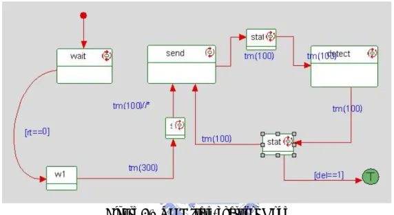
In our simulation, the main part is the node, so we introduce its diagram first. We describe the state chart of the node as the figure 5.1.

Figure 5.1 UML state-chart for Node

In “send” block, the node decides to transmit or not according to its counter and send a different event to the channel. In “detect” block, node detect the channel state and change it attribute according to the channel state and our splitting algorithm. If this node transmits successfully, it will terminate, else it will return the “send” block.

We describe the state chart of the channel as the figure 5.2. The channel is composite with three blocks, “Idle”, “Success” and “Collision”. The “Idle” block will change to the “Success” block if an event of transmitting comes. The “Success” block will change to the “Collision” block if another event of transmitting comes. Each block will change to the “Idle” block when the slot ends.

Chapter 6

Simulation results

To evaluate the performance of “N is known splitting algorithm”, two performance metrics are discussed: system throughput and the average delay of system. The throughput is defined as the number of success packets transmitted in one slot. The average delay is defined as the time from the packet generation to the packet transmitting successfully.

In the Fig. 6.1, the simulation results are obtained by running 1,000,000 time slot, and the average delay is obtained by delay time totalmunber ofsuccess

success

∑

. We compare the average delay of different error rate 0, 0.01, 0.02 and 0.05. For some error rates, we do not measure their average delay with some arrival rates because the average delay is too large. So the expected number of nodes in the system is very large and the simulation time becomes too large.

In Fig.6.1, it can be seen that the average delay is very similar for each error rate at the arrival rate 0.39. But when the arrival rate increases, the average delay of error rate 0.05 increases very fast after the arrival rate 0.40. We can see that the curve of average delay of the error rate 0.01 has a turning point at the arrival rate 0.43. It means that the arrival rate is close to the throughput of the error rate 0.01.

In the Fig. 6.2, the simulation results are obtained by running 10,000 time slot and the throughput is obtained by total success/ 10,000. We compare the throughput of different error rate 0, 0.01, 0.02 and 0.05.

Figure 6.2 Throughput vs. arrival rate of different packet error rate with running time 10,000 time slots.

.

The Fig 6.3 is obtained by the same simulation using in Fig 6.2. It shows the average delay vs. arrival rate of different packet error rate with running time 10,000 time slots. In the Fig. 6.3, the average delay increase very fast when the arrival rate is between 0.4 and 0.6. But the average delay increases slowly when the arrival rate is over than 0.7.

When the arrival rate is near its maximum throughput, each node stays in the system longer and the average delay increases fast. When the arrival rate is over the maximum throughput, some nodes might still stay in the system at the time slot 10,000 and the numbers of these nodes increase when the arrival rate increases. When the arrival rate is between 0.4 and 0.6, most of nodes transmit successfully and add their delay to the total delay. But when the arrival rate is between 0.7 and 1.0, most of nodes will stay in the system. The nodes which have a very large delay might stay in the system but the nodes which have a small delay might transmit successfully because the first-in-first-out is not applied in our algorithm.

Figure 6.3 Average delay vs. arrival rate of different packet error rate with running time 10,000 time slots

Chapter 7

Conclusion

In this thesis, we propose the “N is known splitting algorithm” based on the splitting tree

algorithm. We define a new method to judge CRP for each node and assume that each node can obtain the channel state by itself in our algorithm. In the four cases of the detected error, the cases of 1->e and 1->0 hurt the throughput badly.

In our method, the assumption that N is known by each node is not practical. In the future, we need find a method to estimate the number of nodes which want to send packet.

Reference

[1] Alberto Leon-Garcia and Indra Widjaja, “Communication Networks: fundamental concepts and key architectures” 2nd Ed.

[2] D. Bertsekas et al., Data networks, Englewood Cliffs, NJ: prentice-Hall,1992.

[3] J. Capetanakis, “The Multiple Access Broadcast Channel: Protocol and Capacity Consideration”, IEEE Trans. Infom. Theory, IT-25:505-515, 1979.

[4] X. Wang, Y. Yu and G. B. Giannakis, “A Robust High-Throughput Tree Algorithm Using Successive Interference Cancellation” EEE Transactions on Information Theory, submitted,2005

[5] Y. Yu and G.B. Giannakis, “High-throughput random access using successive interference cancellation in a tree algorithm,” IEEE Transactions on Information Theory, submitted,2005.

[6] M. Sheng, J. Li and F. Jiang, “Hybrid splitting algorithm for wireless MAC,” IEEE Communication Letters, 2005.

[7] X. Qin and R. Berry, “Opportunistic splitting algorithms for wireless networks,” IEEE Infocom, 2004.