IEEE COMMUNICATIONS LETTERS, VOL. 14, NO. 6, JUNE 2010 569
Analytical Model for Wireless Communication Systems
Hung-Hui Juan and ChingYao Huang, Member, IEEE
Abstract—In this paper, a user capacity model, combining
both the modulation and coding scheme (MCS) distribution model and resource allocation model, is developed to analyze the system performance of wireless communication systems. From the model, we can intuitively calculate the system capacity from MCS distribution. An example based on relay networks is used to quantify the benefit of deploying relay stations.
Index Terms—Resource management, mobile communication,
relay networks.
I. INTRODUCTION
I
N future wireless mobile communication systems, some advanced technologies including multi-hop relaying, multiple-input multiple-output (MIMO), femtocell, and etc., are proposed to achieve high transmission rates. With extra implementation costs, it is important to be able to quantify the performance under various deployment scenarios. Issues re-lated to radio resource allocation are addressed in [1]. In [2,3], orthogonal frequency division multiple access (OFDMA) sys-tem based resource allocation is proposed. From [4], the impacts on broadcast channel and capacity are investigated. [5] proposes a rate-and-power based resource allocation algorithm for OFDMA downlink systems. In our work, instead of focus-ing on the resource allocation algorithms, a system resource usage model is established to provide the engineering sense for system deployment and resource allocation. The remaining paper is organized as follows: The proposed analytical model is presented in Section II. In Section III, a two-hop relay network is used as an example to show how to apply the analytical model. Some analysis results are also discussed in Section III. Conclusion is drawn in Section IV.II. PROPOSEDUSERCAPACITYMODEL
The proposed model contains two components including the MCS distribution model and resource allocation model.
A. MCS distribution model
The probability that a mobile station (MS) on the i-level MCS is defined as:
𝑃𝑀𝐶𝑆,𝑖= Pr{MS on i-level MCS Coverage} (1)
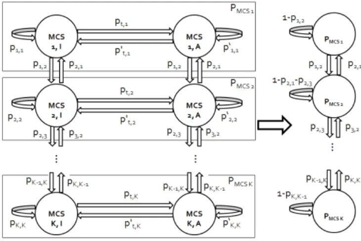
In wireless, with the changing signal quality, the associated MCS assignment will also be changed. To show that, a two dimensional Markov Chain is used. From Fig. 1, the state
Manuscript received February 20, 2009. The associate editor coordinating the review of this letter and approving it for publication was G. Mazzini.
This work was supported in part by the Taiwan ATU Program, NCTU-MediaTek Research Center, and NSC 97-2221-E-009-100-MY3.
The authors are with the National Chiao Tung University, Hsinchu, Taiwan, 300, R.O.C. (e-mail: [email protected], [email protected]).
Digital Object Identifier 10.1109/LCOMM.2010.06.090400
Fig. 1. MCS transition model.
label contains two parameters: The integer number represents the MCS level, and the letter of “I” and “A” means “Idle” and “Active”, respectively. For example, if a MS is transmitting or receiving data based on 64QAM-1/2 coding MCS, then it is labeled as “MCS, 1, A” state. If the MS is in the 16QAM-1/2 coding coverage but is idle, then it is labeled as “MCS, 2, I” state. Due to the MCS setting is mostly based on average channel performance, we assume that the state only jumps to its adjacent states. The state transition probability from i-level to j-level MCS, is𝑝𝑖,𝑗 and𝑝′𝑖,𝑗for “Idle” and “Active” modes,
respectively. And the state transition probability at i-level MCS between “Idle” and “Active” are𝑝𝑡,𝑖and𝑝′𝑡,𝑖. Since the moving
MS from one MCS coverage to another MCS coverage is independent from whether it is in “Idle” or “Active” mode,𝑝𝑖,𝑗
and 𝑝′
𝑖,𝑗 will be equal. With that, we can prove that the two
dimensional Markov chain can be deducted to one dimensional Markov chain; a general proof is provided in Appendix.
B. Resource allocation model
The normalized probability of𝑃𝑀𝐶𝑆,𝑖,𝐴,𝜌𝑖, can be
calcu-lated as:
𝜌𝑖=∑𝐾𝑃𝑀𝐶𝑆,𝑖,𝐴 𝑗=1
𝑃𝑀𝐶𝑆,𝑗,𝐴
(2)
With the 𝜌-factor, we can investigate the transmission
efficiency of radio resources. For the user capacity study, based on a long-term observation, the distribution of MCS, 𝜌1, 𝜌2, . . . 𝜌𝑘 , is stable. For i-level MCS, the number of associated
information bits carried by one resource unit (RU) is defined asbi. We assume that the total number of MSs is N and the maximum number of RU in each downlink sub-frame is𝑈𝐷𝐿.
570 IEEE COMMUNICATIONS LETTERS, VOL. 14, NO. 6, JUNE 2010
Then we can get the following inequality:
𝐾
∑
𝑖=1
𝜌𝑖𝑁𝑅𝜏𝑇𝑓
𝜂𝑖 ≤ 𝜏𝑈𝐷𝐿 (3)
where𝜏 is total frames transmitted, R is the average required
data rate, and𝑇𝑓 is the frame duration.
The inequality (3) can be rewritten as:
𝑁𝑅𝑇𝑓⋅ 𝐾 ∑ 𝑖=1 𝜌𝑖 𝜂𝑖 ≤ 𝑈𝐷𝐿 (4)
If there are M different applications and each has the average required data rate of 𝑅𝑗 and mixed traffic ratio of
for application j, then the inequality (4) can be extended as:
𝑁𝑇𝑓⋅ 𝑀 ∑ 𝑗=1 {𝛽𝑗𝑅𝑗⋅ 𝐾 ∑ 𝑖=1 𝜌𝑗,𝑖 𝜂𝑖 } ≤ 𝑈𝐷𝐿 (5)
where𝜌𝑗,𝑖denotes the normalized station probability of MCS i
for application j. Apparently, the inequality (3-5) indicates that resource constraints will result in a capacity limit. For further performance analysis, we can estimate the user capacity and the maximum system throughput from the proposed model once we know MCS distribution. From inequality (5), the user capacity𝑁∗can then be calculated with the mixture of traffic
types and the distribution in MCS:
𝑁∗= 𝑈𝐷𝐿
𝑇𝑓⋅∑𝑀𝑗=1{𝛽𝑗𝑅𝑗⋅∑𝐾𝑖=1 𝜌𝜂𝑗,𝑖𝑖 }
(6) In the next section, we will show how to compare the user capacity and system throughput of a wireless system with and without the deploying of relay stations.
III. ANEXAMPLEFORRELAYNETWORK
In this section, the user capacity of a wireless two-hop relay network is considered as an example to demonstrate the use of the user capacity model. Without restricting the deployment method of relay stations (RSs), we assume that the proportion of users served by RSs is ˙So, the downlink resource plane can be partitioned into two: one is the resource allocation for the MSs served by macro base station (BS), and the other is the resource allocation for the MSs served by RSs. From inequality (4), the resource allocation for the MSs served by BS and RSs can be written as:
𝑁𝑅𝑇𝑓(1 − 𝛼) ⋅ 𝐾 ∑ 𝑖=1 𝜌𝑖 𝜂𝑖 + 𝑁𝑅𝑇𝑓𝛼 ⋅ ( 𝐾 ∑ 𝑖=1 𝜌𝑅𝑀,𝑖 𝜂𝑖 + 𝐾 ∑ 𝑖=1 𝜌𝐵𝑅,𝑖 𝜂𝑖 ) (7) Here𝜌𝑖is the MCS distribution for BS to MS link,𝜌𝑅𝑀,𝑖is
for RS to MS link, and𝜌𝐵𝑅,𝑖is for BS to RS link, respectively.
Finally, the resource allocation inequality can be written as: 𝑁𝑅𝑇𝑓[(1−𝛼)⋅ 𝐾 ∑ 𝑖=1 𝜌𝑖 𝜂𝑖+𝛼⋅( 𝐾 ∑ 𝑖=1 𝜌𝑅𝑀,𝑖 𝜂𝑖 + 𝐾 ∑ 𝑖=1 𝜌𝐵𝑅,𝑖 𝜂𝑖 )] ≤ 𝑈𝐷𝐿 (8) The first term represents the average number of resource unit used by BS-MS link. The second term presents the average number of resource unit used by RS-MS link, and the third term presents the average number of resource unit used by BS-RS link. For the pure BS network, the resource
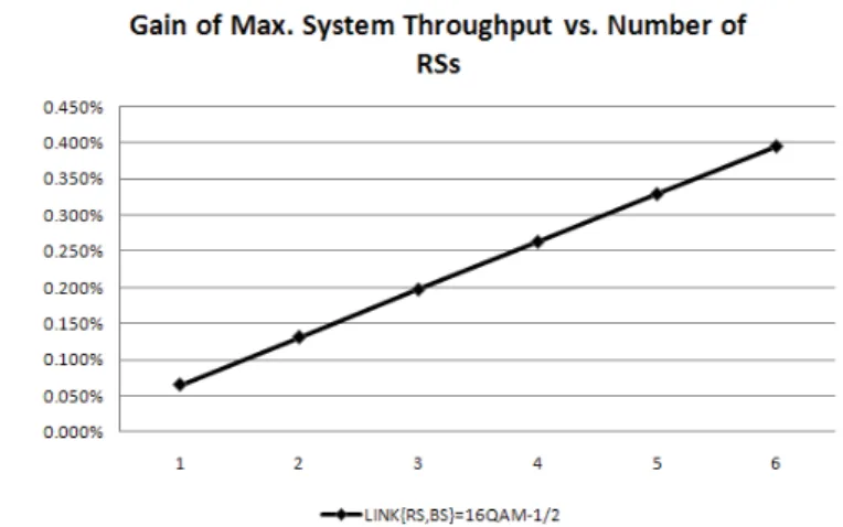
Fig. 2. System throughput gain with BS-RS link of 16QAM-1/2 MCS.
allocation inequality is (4). The user capacity, N*, is calculated in (6) with M=1 (for single application). And the user capacity of the two-hop relay network is (9).
𝑁∗= 𝑈𝐷𝐿 𝑅𝑇𝑓[(1 − 𝛼) ⋅ 𝐾 ∑ 𝑖=1 𝜌𝑖 𝜂𝑖+ 𝛼 ⋅ ( 𝐾 ∑ 𝑖=1 𝜌𝑅𝑀,𝑖 𝜂𝑖 + 𝐾 ∑ 𝑖=1 𝜌𝐵𝑅,𝑖 𝜂𝑖 )] (9)
Moreover, we can estimate the maximum system throughput. Since we assume that the required average data rate of each user is R. The maximum system throughput (MST) (the multiplication of the user number and transmission rates) of the pure BS network and two-hop relay network are calculated in (10) and (11), respectively. 𝑀𝑆𝑇 = 𝑈𝐷𝐿 𝑇𝑓⋅ 𝐾 ∑ 𝑖=1 𝜌𝑖 𝜂𝑖 (10) 𝑀𝑆𝑇 = 𝑈𝐷𝐿 𝑇𝑓[(1 − 𝛼) ⋅ 𝐾 ∑ 𝑖=1 𝜌𝑖 𝜂𝑖 + 𝛼 ⋅ ( 𝐾 ∑ 𝑖=1 𝜌𝑅𝑀,𝑖 𝜂𝑖 + 𝐾 ∑ 𝑖=1 𝜌𝐵𝑅,𝑖 𝜂𝑖 )] (11)
Although the deployment of RSs can help MSs in the cell edge and improve their performance. It also results in transmission redundancy in which BS will first transmit data to RS and then the RS will redirect the data to MS. This redundancy in transmission could potentially degrade the system performance. Compared (10) and (11), the condition that the relay network has better system performance than the pure BS network is shown in (12).
(1−𝛼)⋅ 𝐾 ∑ 𝑖=1 𝜌𝑖 𝜂𝑖+𝛼⋅( 𝐾 ∑ 𝑖=1 𝜌𝑅𝑀,𝑖 𝜂𝑖 + 𝐾 ∑ 𝑖=1 𝜌𝐵𝑅,𝑖 𝜂𝑖 ) ≤ 𝐾 ∑ 𝑖=1 𝜌𝑃 𝑢𝑟𝑒𝐵𝑆,𝑖 𝜂𝑖 (12)
To investigate the performance, we set a simple example for considering only a geographic distribution of MCS as a baseline performance to show the influence of number of RSs and the link quality in between BS and RS. In the analysis, the BS cell radius is 1000 m and the RSs are equally separated and located at the ring of 2/3 cell radius. Three MCSs including 64QAM-1/2, 16QAM-1/2, and QPSK-1/2 are considered. For BS, each MCS has the coverage radius of 200m, 600m, and 1000m, respectively. And for each RS, only 64QAM-1/2 and
JUAN and HUANG: ANALYTICAL MODEL FOR WIRELESS COMMUNICATION SYSTEMS 571
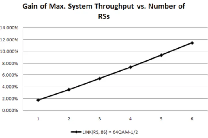
Fig. 3. System throughput gain with BS-RS link of 64QAM-1/2 MCS.
16QAM-1/2 are considered at the coverage radius of 120 m and the coverage radius of 333.33 m.
Figure 2 shows the gain of the system throughput as com-pared to the Pure BS case. We can see that the improvement is less than 1% even with 6 RSs deployed. But from Fig. 3, there is more than 10% of improvement, if the link between RS and BS can be improved to 64QAM-1/2. Apparently, having a better link in between the BS and RS has more impacts on the system performance as compared to adding more RS stations.
IV. CONCLUSION
In this paper, a user capacity model is developed based on MCS distribution model and resource allocation model. The model captures the effect of various applications and most important the MCS distribution. From the two-hop relay example, we can quickly quantify the gain with the changes of RS station number and the link quality in between BS and RS. Furthermore, the capacity model can be adopted by consid-ering QoS constraints, scheduling and advanced technologies like MIMO and beam forming which can potentially change the MCS distribution and the transmitted rates per RU.
APPENDIXA
Here we will show that the two dimensional Markov chain can be deducted to one dimensional Markov chain. As a result, the state probability, 𝑃𝑀𝐶𝑆,𝑖, depending only on transition
probability. The state probability,𝑃𝑀𝐶𝑆,𝑖, can be expressed
as: 𝑃𝑀𝐶𝑆,𝑖≡ 𝑃𝑀𝐶𝑆,𝑖,𝐼+ 𝑃𝑀𝐶𝑆,𝑖,𝐴 For i = 1, 𝑃𝑀𝐶𝑆,1,𝐼= 𝑝1,1⋅ 𝑃𝑀𝐶𝑆,1,𝐼+ 𝑝2,1⋅ 𝑃𝑀𝐶𝑆,2,𝐼+ 𝑝′𝑡,1⋅ 𝑃𝑀𝐶𝑆,1,𝐴 𝑃𝑀𝐶𝑆,1,𝐴= 𝑝′1,1⋅ 𝑃𝑀𝐶𝑆,1,𝐴+ 𝑝2,1⋅ 𝑃𝑀𝐶𝑆,2,𝐴+ 𝑝𝑡,1⋅ 𝑃𝑀𝐶𝑆,1,𝐼 𝑃𝑀𝐶𝑆,1= 𝑃𝑀𝐶𝑆,1,𝐼+ 𝑃𝑀𝐶𝑆,1,𝐴 = 𝑝2,1⋅ (𝑃𝑀𝐶𝑆,2,𝐼+ 𝑃𝑀𝐶𝑆,2,𝐴) + (𝑝1,1+ 𝑝𝑡,1) ⋅ 𝑃𝑀𝐶𝑆,1,𝐼+ (𝑝′1,1+ 𝑝′𝑡,1) ⋅ 𝑃𝑀𝐶𝑆,1,𝐴 given𝑝1,1+ 𝑝𝑡,1+ 𝑝1,2= 1 and 𝑝′1,1+ 𝑝′𝑡,1+ 𝑝1,2= 1 𝑃𝑀𝐶𝑆,1= 𝑝2,1⋅ 𝑃𝑀𝐶𝑆,2+ (1 − 𝑝1,2) ⋅ 𝑃𝑀𝐶𝑆,1,𝐼+ (1 − 𝑝1,2) ⋅ 𝑃𝑀𝐶𝑆,1,𝐴 = 𝑝2,1⋅ 𝑃𝑀𝐶𝑆,2+ (1 − 𝑝1,2) ⋅ 𝑃𝑀𝐶𝑆,1 For1 < 𝑖 < 𝐾, 𝑃𝑀𝐶𝑆,𝑖,𝐼= 𝑝𝑖−1,𝑖⋅ 𝑃𝑀𝐶𝑆,𝑖−1,𝐼+ 𝑝𝑖,𝑖⋅ 𝑃𝑀𝐶𝑆,𝑖,𝐼+ 𝑝𝑖+1,𝑖⋅ 𝑃𝑀𝐶𝑆,𝑖+1,𝐼+ 𝑝′ 𝑡,𝑖⋅ 𝑃𝑀𝐶𝑆,𝑖,𝐴 𝑃𝑀𝐶𝑆,𝑖,𝐴= 𝑝𝑖−1,𝑖⋅𝑃𝑀𝐶𝑆,𝑖−1,𝐴+𝑝′𝑖,𝑖⋅𝑃𝑀𝐶𝑆,𝑖,𝐴+𝑝𝑖+1,𝑖⋅𝑃𝑀𝐶𝑆,𝑖+1,𝐴+ 𝑝𝑡,𝑖⋅ 𝑃𝑀𝐶𝑆,𝑖,𝐼 𝑃𝑀𝐶𝑆,𝑖= 𝑃𝑀𝐶𝑆,𝑖,𝐼+ 𝑃𝑀𝐶𝑆,𝑖,𝐴 𝑃𝑀𝐶𝑆,𝑖= 𝑝𝑖−1,𝑖⋅𝑃𝑀𝐶𝑆,𝑖−1+𝑝𝑖+1,𝑖⋅𝑃𝑀𝐶𝑆,𝑖+1+(𝑝𝑖,𝑖+𝑝𝑡,𝑖)⋅𝑃𝑀𝐶𝑆,𝑖,𝐼+ (𝑝′ 𝑖,𝑖+ 𝑝′𝑡,𝑖) ⋅ 𝑃𝑀𝐶𝑆,𝑖,𝐴 = 𝑝𝑖−1,𝑖⋅𝑃𝑀𝐶𝑆,𝑖−1+𝑝𝑖+1,𝑖⋅𝑃𝑀𝐶𝑆,𝑖+1+(1−𝑝𝑖,𝑖+1+𝑝𝑖,𝑖−1)⋅(𝑃𝑀𝐶𝑆,𝑖,𝐼+ 𝑃𝑀𝐶𝑆,𝑖,𝐴) = 𝑝𝑖−1,𝑖⋅ 𝑃𝑀𝐶𝑆,𝑖−1+ 𝑝𝑖+1,𝑖⋅ 𝑃𝑀𝐶𝑆,𝑖+1+ (1 − 𝑝𝑖,𝑖+1+ 𝑝𝑖,𝑖−1) ⋅ 𝑃𝑀𝐶𝑆,𝑖 For𝑖 = 𝐾 𝑃𝑀𝐶𝑆,𝐾,𝐼= 𝑝𝐾−1,𝐾⋅𝑃𝑀𝐶𝑆,𝐾−1,𝐼+𝑝𝐾,𝐾⋅𝑃𝑀𝐶𝑆,𝐾,𝐼+𝑝′𝑡,𝐾⋅𝑃𝑀𝐶𝑆,𝐾,𝐴 𝑃𝑀𝐶𝑆,𝐾,𝐴= 𝑝𝐾−1,𝐾⋅𝑃𝑀𝐶𝑆,𝐾−1,𝐴+𝑝′𝐾,𝐾⋅𝑃𝑀𝐶𝑆,𝐾,𝐴+𝑝𝑡,𝐾⋅𝑃𝑀𝐶𝑆,𝐾,𝐼 𝑃𝑀𝐶𝑆,𝐾= 𝑃𝑀𝐶𝑆,𝐾,𝐼+ 𝑃𝑀𝐶𝑆,𝐾,𝐴 = 𝑝𝐾−1,𝐾⋅ 𝑃𝑀𝐶𝑆,𝐾−1+ (1 − 𝑝𝐾,𝐾−1) ⋅ 𝑃𝑀𝐶𝑆,𝐾,𝐼+ (1 − 𝑝𝐾,𝐾−1) ⋅ 𝑃𝑀𝐶𝑆,𝐾,𝐴 = 𝑝𝐾−1,𝐾⋅ 𝑃𝑀𝐶𝑆,𝐾−1+ (1 − 𝑝𝐾,𝐾−1) ⋅ (𝑃𝑀𝐶𝑆,𝐾,𝐼+ 𝑃𝑀𝐶𝑆,𝐾,𝐴) For all i, the steady state probability of the new one dimen-sional Markov chain,𝑃𝑀𝐶𝑆,𝑖, depends only on the transition
probability and state probabilities. Q.E.D. REFERENCES
[1] L. Jorguseki, J. Farserotu, and R. Prasad, “Radio resource allocation in third-generation mobile communication systems,” IEEE Commun. Mag., vol. 39, no. 2, pp. 117-23, Feb. 2001.
[2] S. Pietrzyk and G. J. M. Janssen, “Multiuser subcarrier allocation for QoS provision in the OFDMA systems,” in Proc. IEEE Veh. Technol. Conf., vol. 2, Sep. 2002, pp. 1077-1081.
[3] M. Ergen, S. Coleri, and P. Varaiya, “QoS aware adaptive resource allocation techniques for fair scheduling in OFDMA based broadband wireless access systems,” IEEE Trans. Broadcast., Dec. 2003. [4] L. Li and A. Goldsmith, “Capacity and optimal resource
alloca-tion for fading broadcast channels—part I: ergodic capacity,” IEEE Trans. Inf. Theory, vol. 47, pp. 1083-1102, Mar. 2001.
[5] K. Seong, M. Mohseni, and J. M. Cioffi, “Optimal resource allocation for OFDMA downlink systems,” in IEEE ISIT, 2006.