以微觀力學模式模擬複合材料與應變率有關之非線性行為
124
0
0
全文
(2) 以微觀力學模式模擬複合材料與應變率有關之非線性行為 Modeling Nonlinear Rate Dependent Behavior of Composites Using Micromechanical Approach 研 究 生:陳奎翰. Student:Kuei-Han Chen. 指導教授:蔡佳霖. Advisor:Jia-Lin Tsai. 國. 立. 交. 通. 大. 學. 機 械 工 程 系 碩 士 論 文 A Thesis Submitted to Department of Mechanical Engineering College of Engineering National Chiao Tung University in partial Fulfillment of the Requirements for the Degree of Master in Mechanical Engineering July 2005 Hsinchu, Taiwan, Republic of China. ㆗ 華 民 國 九 十 ㆕ 年 七 月.
(3) 以微觀力學模式模擬複合材料 與應變率有關之非線性行為 學生:陳奎翰. 指導教授:蔡佳霖. 國立交通大學機械工程學系碩士班 摘. 要. 本研究目的在於以微觀力學模式描繪碳纖/環氧樹脂複合材料與應變 率有關之非線性行為。材料性質方面,將環氧樹脂假設為彈性黏塑性材料 並以㆔參數黏塑性模式描述之,纖維則假設為橫向等向性材料。藉由環氧 樹脂在 10-4、10-2 以及 1/s ㆔種應變率之㆘的壓縮試驗,㆔參數模式所需的 係數可藉由實驗獲得的應力應變曲線來定義。伴隨著已知的碳纖與環氧樹 脂的材料性質,碳纖/環氧樹脂複合材料可藉由微觀力學模式進行模擬。在 此研究㆗,有兩個微觀力學模式被採用,分別是 Square Fiber Model 以及 Generalized Method of Cells。此外,兩種纖維排列方式(Square Edge Packing 與 Square Diagonal Packing)與兩種纖維形狀(圓形與正方形)被㆒併考量 並且與 ANSYS 所執行之有限元素法做㆒系列纖維排列與纖維形狀對材料 性質影響性的比較與探討。數值結果指出纖維形狀對偏軸複合材料機械性 質的影響並不明顯,然而,纖維的排列方式對此卻有顯著的影響性,而且 Square Edge Packing 相較於 Square Diagonal Packing 模擬出更硬的應力應變 曲線。 i.
(4) 為了驗證微觀力學模式的準確性,偏軸的碳纖/樹脂複材試片在 10-4 到 550/s 的應變率之㆘做壓縮測試以獲得實驗值。由實驗值與模式預測的比較 結果可知,數值預測結果雖然與實驗有㆒定程度的差異,但結合㆔參數黏 塑性模式的微觀力學模式的確有能力描述與應變率有關的材料非線性行 為。. ii.
(5) Modeling Nonlinear Rate Dependent Behavior of Composites Using Micromechanical Approach Student:Kuei-Han Chen. Advisor:Dr. Jia-Lin Tsai. Institute of Mechanical Engineering. National Chiao Tung University. Abstract This research aims to characterize the nonlinear rate dependent behavior of graphite/epoxy composites using a micromechanical approach.. For epoxy phase, it was. assumed to be following the elastic/viscoplastic behavior described by a three parameterts viscoplasticity model; while the graphite fiber was assumed to be a transverse isotropic solid. By performing compression tests on the epoxy resin at three different strain rates of 10-4, 10-2 and 1/s, the stress and strain relation of the epoxy resin was generated. Based on the experimental data, the three parameter viscoplasticity model was developed.. With the. ingredient properties, the mechanical behaviors of graphite/epoxy composites were characterized using the micromechanical approach.. There are two micromechanical models,. i.e. Generalized Method of Cell (GMC) and Square Fiber Model (SFM), were employed in this study. In addition, two different fiber arrangements, i.e., square edge packing and square iii.
(6) diagonal packing as well as the fiber shapes, i.e. square type and round type, were taken into account.. The finite element analysis with commercial code ANSYS was also adopted to. investigate the fiber arrangement effect and the fiber shape effect.. It was indicated basically,. the mechanical behaviors were not affected appreciably by the fiber shape.. On the contrary,. the fiber arrangements play an essential role on the mechanical behaviors.. The square edge. packing demonstrates stiffer behaviors than the square diagonal packing.. In order to verify. the model predictions, off-axis graphite/epoxy composite specimens were tested at strain rate ranges from 10-4/s to 550/s.. Comparison of model predictions obtained from GMC and SFM. analysis with the experimental results revealed that the micromechanical approaches are capable of predicting the nonlinear rate sensitivity of off-axis specimens although there are still distinctions between the model and the experimental results.. iv.
(7) 誌謝 此文,謹獻給伴我走過碩士生涯的師長、同學、朋友們。 兩年前,我帶著無知與懵懂進入交通大學機械系碩士班追隨蔡佳霖博士從事複合材 料研究,從㆒名專業知識停留在大學程度的毛頭小子,藉由研究所課程的訓練與洗禮, 逐漸培養出正確積極的研究態度與充足的專業知識,進而蛻變為具獨當㆒面處理、解決 問題能力的碩士生。這段改變歷程固然艱苦,但品嚐到豐收果實的霎時間,㆒切辛苦都 是值得的,畢竟,要怎麼收穫,先那麼栽。 在此,我誠摯㆞向兩年來在各方面支持我的㆟們致㆖由衷的感謝。感謝指導教授蔡 佳霖老師,俗話說「㆒日為師終身為父」,謝謝老師您兩年來的指導,無私㆞傳授我們 研究的方法與專業知識,讓我對複合材料有深層且深刻的認識,生活㆖也蒙您照顧,使 實驗室雖經風浪也能㆒路安穩度過。老師,謝謝您。 感謝使我衣食無缺無後顧之憂的父母,你們不肖的兒子離家求學九年,未曾替家盡 過㆒份心力,願我入伍服役後學會成熟、負責以及爸爸您希望我體悟的服從,早日替家 庭負擔生計。感謝前女友筱婷,雖然離別使我的生活頓失重心與依靠,但這段日子,我 熬過來了,相信在遠方的妳也默默㆞為我祝福並希望我也同妳㆒般過得好。感謝馥,陪 伴我最後㆔個月的研究所生涯,每逢週末的郊遊踏青、小酌閒談,是研究所後期最快樂 的時光。 感謝兩位已畢業的學長漢偉與仁傑,將剛進實驗室的我帶㆖軌道,去年你們畢業 時,我擔心自己的能力不足以接掌實驗室負責㆟以及引領學弟們,㆒年後,雖不臻完美 卻也㆗規㆗矩。感謝同學濬清在畢業前夕苦熬著偏軸複材的壓縮試驗,提供㆒組近乎完 美的實驗數據給我的微觀力學模型使用,沒有你的實驗配合,這本論文無法稱為完整。 感謝同學世民給我不少試片製作㆖的觀念與技術,尤其在樹脂除氣與模具的使用㆖,提 供了莫大的協助。感謝學弟明道與世華,在我研究苦悶之際給予精神㆖的支持與提供排 憂解愁的管道。 最後,特別感謝明安國際朱國棟博士、清華大學葉孟考教授與㆗正大學黃崧任博士 於百忙㆗抽空擔任學位論文口試委員並給予論文內容甚多建議,使此論文更趨完善與正 確。此外,感謝工研院材料所的盧廷鉅學長與德霖技術學院邱進東博士分別教導我 ABAQUS 與 MARC 的基礎操作,雖然這兩套軟體最後沒為我的論文所採用,但能順利 得到有限元素法的分析成果,㆓位功不可沒。 欲感謝之㆟眾多,恐有疏漏,在此致㆖歉意並於文末㆒道感謝,感謝㆒路陪我走來 的眾㆟,謝謝你們。. 陳奎翰 2005.07.19 於交通大學. v.
(8) 目. 錄. ㆗文摘要. ………………………………………………………………………………. i. 英文摘要. ………………………………………………………………………………. iii. 誌謝. ………………………………………………………………………………. v. 目錄. ………………………………………………………………………………. vi. 表目錄. ……………………………………………………………………………… viii. 圖目錄. ……………………………………………………………………………… viii. Chapter 1. Introduction…………………………………………………………………. 1. 1.1 Research Motive………………………………………………………. 1. 1.2 Paper Review…………………………………………………………. 1. 1.3 Research Approach……………………………………………………. 6. Chapter 2. Polymer Modeling…………………………………………………………. 7. 2.1 Experiments……………………………………………………………. 7. 2.1.1 Compression Test…………………………………………………. 7. 2.1.2 Tensile Test………………………………………………………. 8. 2.1.3 Measurement of Coefficient of Thermal Expansion………………. 9. 2.2 Visco-Plasticity Model…………………………………………………. 12. 2.3 Modeling of Split Hopkinson Pressure Bar Results……………………. 16. Chapter 3. Square Fiber Model…………………………………………………………. 18. 3.1 Square Fiber Model……………………………………………………. 18. 3.2 Modified Square Fiber Model…………………………………………. 24. 3.2.1 Square Edge Packing Array………………………………………. 24. 3.2.2 Square Diagonal Packing Array…………………………………. 28. Chapter 4. Generalized Method of Cells………………………………………………. 33. 4.1 Generalized Method of Cells (GMC)…………………………………. 33. Chapter 5. Finite Element Analysis……………………………………………………. 48. 5.1 Finite Element Approach………………………………………………. 48. Chapter 6. Results and Discussion……………………………………………………. 53. 6.1 Thermal Stress Effect…………………………………………………… 53. vi.
(9) 6.2 Discussion of Fiber Shape and Fiber Arrangement Effect……………. 55. 6.2.1 Fiber Shape Effect………………………………………………… 55 6.2.2 Fiber Arrangement Effect………………………………………… 56 6.3 Comparing with Experimental Data……………………………………. 57. Chapter 7. Conclusion…………………………………………………………………. 60. Reference ………………………………………………………………………………. 61. Appendix A A MATLAB Code for Square Fiber Model………………………………… 65 Appendix B A MATLAB Code for Generalized Method of Cells………………………. vii. 70.
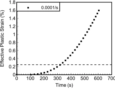
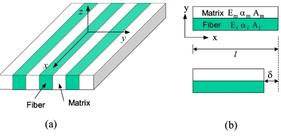
(10) LIST OF TABLES Table01.. Table02.. Material properties used in the micromechanical analysis where the matrix properties were obtained from experiments and the fiber properties were determined to fit the linear elastic of experimental data at all off-axis angles.....78 Material properties employed in the finite element analysis................................78. LIST OF FIGURES Fig. 2.1 Fig. Fig. Fig. Fig. Fig. Fig. Fig.. 2.2 2.3 2.4 2.5 2.6 2.7 2.8. Fig. 2.9 Fig. Fig. Fig. Fig.. 2.10 2.11 2.12 2.13. Fig. 3.1 Fig. 3.2 Fig. 3.3 Fig. 3.4. Fig. 3.5 Fig. 3.6 Fig. 4.1 Fig. 4.2 Fig. 4.3. Dimensions of tensile and compression specimens. (a) Cylindrical compression specimen. (b) Coupon tensile specimen………………………… 79 Experimental setup for compression tests…………………………………….. 79 Compression test results of polymer at 10-4, 10-2 and 1/s strain rates………… 80 Tensile test result to determine Poisson’s ratio of the polymer……………….. 80 Schematic for a strain gage subjected to a biaxial strain field………………… 81 A half-bridge circuit for measuring the coefficient of thermal expansion……. 81 Thermal response for the polymer…………………………………………….. 82 Effective stress – effective plastic strain curves for polymer at three different strain rates……………………………………………………………………... 82 Effective plastic strain versus time curve for epoxy at strain rate of 10-4/s…… 83 Log-log plot for determining the parameters in the viscoplasticity model……. 83 The stress – strain curve of the polymer from SHPB results………………….. 84 The stress – time curve from SHPB test………………………………………. 84 Prediction results of polymer at different strain rates by using three parameters model……………………………………………………………… 85 Demonstration of RVEs with various fiber arrangements. (a) Square edge packing array. (b) Square diagonal packing array…………………………….. 86 Geometry of square fiber model………………………………………………. 86 Square edge packing array for modified square fiber model………………….. 87 Fiber distribution of square diagonal packing array (SDP) based on the fiber volume fraction. (a) Less than 39.3 %. (b) Equal to 39.3 %. (c) Greater than 39.3 %. (d) Attain to maximum fiber volume fraction 78.5 %………………... 87 Square diagonal packing array for modified square fiber model……………... 88 Two fiber phases can be treated as a whole one if the constant stress or strain assumptions in eqn (3.2.21) were applied…………………………………….. 88 The coordinate system and geometry information of the generalized method of cells…………………………………………………………………………. 89 Local coordinate systems of the generalized method of cells………………… 89 Normal vectors at the interfaces of subcells…………………………………... 90 viii.
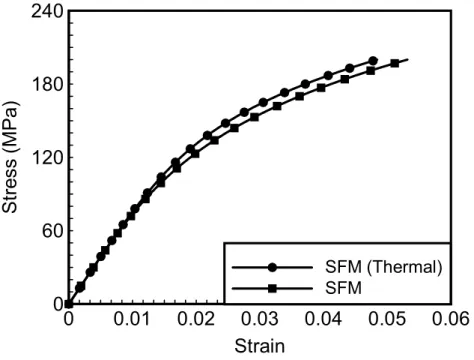
(11) Fig. 4.4 Fig. 5.1 Fig. 5.2 Fig. 5.3 Fig. 6.1. Fig. 6.2. Fig. 6.3. Fig. 6.4 Fig. 6.5 Fig. 6.6. Fig. 6.7 Fig. 6.8. A four regions RVE employed in the GMC, in which β = γ = 1 represents the fiber phase…………………………………………………………………. 90 3-D square diagonal packing array employed in ANSYS…………………….. 91 (a)A finite element mesh generated by ANSYS………………………………. 91 (b)A full view of finite element mesh…………………………………………. 92 An assumed stress–strain curve of the matrix………………………………… 92 (a) Simplified model for unidirectional fiber composites. (b) Evaluation of thermal residual stress based on the displacement continuity in the x direction…………………………………………………………… 93 (a)Thermal stress effect on the stress and strain curve of 300 fiber composite obtained from the square fiber model……………………………………… 93 (b)Thermal stress effect on the stress and strain curve of 900 fiber composite obtained from the square fiber model……………………………………… 94 (a)Thermal stress effect on the stress and strain curve of 300 fiber composite obtained from the generalized method of cells…………………………….. 94 (b)Thermal stress effect on the stress and strain curve of 900 fiber composite obtained from the generalized method of cells……….……………………. 95 The RVE with 26 × 26 subcells employed in the calculation of generalized method of cells (square edge packing)………………………………………... 95 The RVE with 50 subcells in fibrous region employed in the modified square fiber model (square edge packing)……………………………………………. 96 (a)Fiber shape effects on the stress and strain curves of 150 fiber composites using the generalized method of cells (GMC) and the square fiber model (SFM)………………………………………………………………………. 96 (b)Fiber shape effects on the stress and strain curves of 300 fiber composites using the generalized method of cells (GMC) and the square fiber model (SFM)………………………………………………………………………. 97 (c)Fiber shape effects on the stress and strain curves of 450 fiber composites using the generalized method of cells (GMC) and the square fiber model (SFM)………………………………………………………………………. 97 (d)Fiber shape effects on the stress and strain curves of 600 fiber composites using the generalized method of cells (GMC) and the square fiber model (SFM)………………………………………………………………………. 98 The RVE with 20 × 20 subcells employed in the calculation of generalized method of cells (square diagonal packing)……………………………………. 98 The RVE employed in the modified square fiber model (square diagonal packing)……………………………………………………………………….. 99. ix.
(12) Fig. 6.9. Fig. 6.10. Fig. 6.11. Fig. 6.12. (a)The effect of fiber arrangements on the stress and strain curves of 150 fiber composites obtained from the SFM and GMC………………………….…. 99 (b)The effect of fiber arrangements on the stress and strain curves of 300 fiber composites obtained from the SFM and GMC……………………... 100 (c)The effect of fiber arrangements on the stress and strain curves of 450 fiber composites obtained from the SFM and GMC……………………... 100 (d)The effect of fiber arrangements on the stress and strain curves of 600 fiber composites obtained from the SFM and GMC……………………... 101 (a)The effect of fiber arrangements on the stress and strain curves of 150 fiber composites obtained from the FEM………………………………… 101 (b)The effect of fiber arrangements on the stress and strain curves of 300 fiber composites obtained from the FEM………………………………… 102 (c)The effect of fiber arrangements on the stress and strain curves of 450 fiber composites obtained from the FEM………………………………… 102 (d)The effect of fiber arrangements on the stress and strain curves of 600 fiber composites obtained from the FEM………………………………… (a)Comparison of the stress and strain curves of 150 fiber composites with square edge packing array obtained from FEM, SFM and GMC………... (b)Comparison of the stress and strain curves of 300 fiber composites with square edge packing array obtained from FEM, SFM and GMC………... (c)Comparison of the stress and strain curves of 450 fiber composites with square edge packing array obtained from FEM, SFM and GMC………... (d)Comparison of the stress and strain curves of 600 fiber composites with square edge packing array obtained from FEM, SFM and GMC………... (e)Comparison of the stress and strain curves of 150 fiber composites with square diagonal packing array obtained from FEM, SFM and GMC……. (f)Comparison of the stress and strain curves of 300 fiber composites with square diagonal packing array obtained from FEM, SFM and GMC……. (g)Comparison of the stress and strain curves of 450 fiber composites with square diagonal packing array obtained from FEM, SFM and GMC……. (h)Comparison of the stress and strain curves of 600 fiber composites with square diagonal packing array obtained from FEM, SFM and GMC……. (a)Comparison of the experimental data with the model prediction obtained from SFM for 150 fiber composites………………………………………. (b)Comparison of the experimental data with the model prediction obtained from SFM for 300 fiber composites………………………………………. (c)Comparison of the experimental data with the model prediction obtained from SFM for 450 fiber composites………………………………………. x. 103 103 104 104 105 105 106 106 107 107 108 108.
(13) Fig. 6.13. (d)Comparison of the experimental data with the model prediction obtained from SFM for 600 fiber composites………………………………………. (a)Comparison of the experimental data with the model prediction obtained from GMC for 150 fiber composites……………………………………... (b)Comparison of the experimental data with the model prediction obtained from GMC for 300 fiber composites……………………………………... (c)Comparison of the experimental data with the model prediction obtained from GMC for 450 fiber composites……………………………………... (d)Comparison of the experimental data with the model prediction obtained from GMC for 600 fiber composites…………………………………….... xi. 109 109 110 110 111.
(14) Chapter 1 Introduction 1.1 Research Motive Composite materials, because of their high strength/weight ratio, have been extensively used not only in aerospace industry but also in marine and automotive industries. In some of the applications, high strain rate loading may be produced, such as blast loading of a submarine hull and bird strike of an aircraft structure. Thus characterizing and modeling the high strain rate responses of composite materials is becoming an essential task for further applications.. It is well known that. the polymeric materials exhibit nonlinear rate dependent behavior, which implies that the polymeric composite will somehow exhibit the rate sensitivity if the associated behavior is dominated by the matrix.. In past decades, the nonlinear rate dependent. behavior of composites have been studied by many researchers who treated the unidirectional composites as orthotropic homogeneous solids. macro-mechanical analysis.. This is so called. However, in this macro-mechanical approach, the. mechanism of how the fiber and the matrix material affect the overall composite nonlinearity can not be fully characterized.. Therefore, a research from the. micromechanical viewpoint was proposed and used to investigate this phenomenon. In the micromechanical approach, the fiber arrangement, the fiber shape, fiber properties and matrix properties were taken into account and the effect of the ingredients on the rate sensitivity of the composites were further examined.. 1.2 Paper Review Unidirectional fiber composite materials exhibit nonlinear rate dependent behavior under off-axis loading.. There are two points of view to discuss this. physical phenomenon, i.e. macromechanical and micromechanical mechanics, and all published literatures originated from either of the two perspectives. Based on the 1.
(15) viewpoint of macromechanics, Sun and Chen [1] developed a single parameter yield function under plane stress assumption and brought it into the flow rule with a power law curve fitting effective stress – effective plastic strain relation to describe the nonlinearity of fiber composites. This single parameter in the yield function was chosen suitably so that all off-axis experimental data collapse into a single master curve in the effective stress versus effective plastic strain domain.. It is a fact that the. single parameter model has good agreements with experiments. Because of rate independence in this model, some improvements were carried out.. Gates and Sun [2]. combined the over stress model [3] with the single parameter model to predict the rate dependent behavior of composites under loading (the over stress is positive) and unloading (the over stress is zero) conditions. In order to use the over stress model, a quasistatic stress - strain relation was set as a reference state, and when the strain rate is higher, the corresponding relative effective stress was calculated by subtracting the quasistatic effective stress from the current effective stress associated with the same strain level.. The relative effective stress and effective plastic strain rate. relations obtained from the over stress model were then employed together with the flow rule for characterizing the plastic deformation of composites subjected off-axis loading.. Yoon and Sun [4] used the same way as Gates and Sun [2] to investigate. the effects of variant strain rates on a monotonic tension process under off-axis loading.. The results were also compared with a modified Bodner and Partom’s. model [5].. Weeks and Sun [6] modeled off-axis composites using a mathematical. form similar to Johnson-Cook model [7] in conjunction with the single parameter model.. A quasistatic state was chosen as a reference state to get the corresponding. reference effective plastic strain rate and effective stress while the Johnson-Cook model was working.. Then, the effective stress and effective plastic strain rate. relation at high strain rate analyses could be obtained via this model and applied into 2.
(16) flow rule to get corresponding plastic responses like the over stress model. Thiruppukuzhi and Sun [8] directly introduced a rate dependent term into the effective stress – effective plastic strain power law relation and proposed a three parameters model for modeling the nonlinear rate dependent behavior of unidirectional fiber composites. Since the power law equation is a convenient form to use, in this study, the three parameters model was adopted as the viscoplasticity model to describe the rate dependent nonlinearity of the matrix phase. In order to investigate the nonlinear effect of matrix on the mechanical behavior of fiber composites, a micromechanical approach is proposed by modeling the composites as heterogeneous solids consisting of fiber and matrix phases. Through the characteristics of repetition, a Representative Volume Element (RVE) was selected to represent the whole composite materials.. By analyzing the. mechanical behavior of the RVE, the overall material responses of composites could be determined.. There are several micromechanical models available for describing. the mechanical behaviors of composites, i.e., Eshelby model [9], Mori-Tanaka model [10,11], square fiber model [12] and generalized method of cells [13-15].. Eshelby [9]. introduced Eshelby’s tensor together with the equivalent principal concept to model a homogeneous inclusion embedded in an infinite matrix.. Basically, Eshelby model is. a dilute model because only one inclusion is considered. Mori and Tanaka [10] extended Eshelby’s approach to establish a non-dilute model in which the stress and strain states of the inclusion and the matrix were considered in an average sense. Benveniste [11] gave alternative explanations of Eshelby model and Mori-Tanaka model by introducing the strain concentration concept and obtained succinct formulas for these two models.. Commonly, the Eshelby model and Mori-Tanaka model were. mainly applied to characterize the stiffness of short fiber composites. However, they could be extended to characterize the long fiber composites if the aspect ratio of the 3.
(17) inclusion was assumed to be infinity [16] and the nonlinear behavior of composites can be described if an incremental Mori-Tanaka mean field approach was adopted [17]. Sun and Chen [12] proposed a “Square Fiber Model” constructed by a RVE composed of one square fiber and two pure matrix regions.. A 2-D plane stress. plastic potential modified from von Mises J2 function was applied in conjunction with the associated flow rule to describe the plastic strain of the matrix material, while the fiber was regarded as an orthotropic elastic material.. The entire stiffness matrix of. the composite was derived from some suitable constant stress and constant strain assumptions between each subcell in the RVE.. Therefore, we can obtain the total. strain increments due to a given stress history by using this model.. Similar to this. way, Goldberg and Stouffer [18] suggested a four regions model with one square fiber and three matrix regions.. Not a plane stress condition but both two transverse. directions have to be applied constant stress and strain assumptions in all subregions to obtain the overall constitutive equation.. The matrix phase was described using the. Bodner and Partom’s model [5] and the corresponding deformation was solved by using the Runge-Kutta method. Away from the forgoing theories, Aboudi [13, 14] derived a four regions micro-mechanical model called “Method of Cells”, which is very efficient in modeling the elastic and inelastic behavior of fiber-reinforced unidirectional composites. Based on the displacement and traction continuity at the interfaces of all subcells as well as the periodicity at the RVE, a stress - strain relation was described in a matrix form to predict mechanical behavior of composite materials. By extending the method of cells, Paley and Aboudi [15] proposed a scheme called Generalized Method of Cells (GMC) which can deal with an undetermined numbers of subcells.. The weak point in GMC is that the more subcells you have, the more. CPU time is required. To enhance computational efficiency of GMC, Orozco [19] took advantage of the sparse features of the strain concentration matrix. 4. It is.
(18) basically an improvement in the numerical processing.. The sparse implementation. of GMC made it possible to solve the problems with complex micro-structures and tiny refinements.. Pindera and Bednarcyk [20] adopted a different manner to enhance. the computational efficiency of GMC.. They expressed the displacement continuity. between the subcells in terms of stresses and then derived a modified formulation of GMC.. This formulation is regarded as the most efficient way in the employment of. GMC until now. The feature of the GMC is that which cells were fibers or matrices were not indicated in advance.. In other words, we can assign the cells with either. fibers or matrix after forward when the final constitutive equation was established. In applications of the GMC, Orozco and Pindera [21] combined the GMC with an available tangent plasticity matrix to analyze transverse mechanical behavior of composites under different fiber arrangements and fiber shapes.. A large number of. subcells were constructed in their study to model the complex microstructures. It showed that different fiber arrangements and fiber shapes lead to distinct constitutive behavior. Ogihara et al. [22] characterized the nonlinear behavior of carbon/epoxy unidirectional and angle-ply laminates. The GMC was applied first to obtain the property of unidirectional fiber composites under off-axis loading.. Together with the. laminate plate theory, the angle-ply laminates were calculated from the unidirectional composites. Kawai et al. [23] investigated the AS4/PEEK composites under loading and unloading conditions on the off-axis response at strain rate up to 0.01/min.. The. PEEK matrix was described by Chaboche model and the composite was predicted using GMC.. The results showed good agreements with the experimental results for. AS4/PEEK composites.. However, the strain rates in their investigation were not. high enough for engineering applications. Using finite element analysis, Zhu and Sun [24] investigated the nonlinear behaviors of fiber composites by applying suitable boundary conditions on a RVE selected properly with three different fiber 5.
(19) arrangements.. It was shown that the square diagonal packing array provides the best. prediction on the experimental results for all samples with various off-axis angles. 1.3 Research Approach In view of the forgoing, most of efforts were made on the nonlinear behaviors of fiber composites.. While very few studies concerning the rate effect on the. constitutive behaviors were reported. Therefore, this research aims to characterize the nonlinear rate dependent behavior of graphite/epoxy composites.. More. emphases will be placed on the combination effect of microstructure and strain rate. As a result, a micromechanical model consisting of fiber and matrix phases together with their respective constitutive relations will be employed for this analysis. It is noted that the fiber phase was assumed as transverse isotropic elastic materials.. For. matrix phase, the cylindrical specimens were tested in compression on a MTS system to characterize its rate dependent behavior.. Based on the experimental results, the. three parameters model [8] was employed to describe the rate sensitivity of the matrix material. With the matrix and fiber constitutive curves, the micromechanical models will be implemented for modeling the nonlinearity of the fiber composites. It is noted that there were two different micromechanical models utilized in this analysis, i.e. Square Fiber Model (SFM) [12] and Generalized Method of Cells (GMC) [15]. The effect of the fiber arrangements and fiber shapes will be taken into account in the micromechanical modeling together with the finite element method (FEM) and the results will be compared to one another. In addition, the effect of thermal residual stresses are also involved in the analysis.. Finally, the square fiber embedded in the. RVE with square edge packing array was performed using SFM and GMC and has a comparison to the experimental results obtained by testing off-axis graphite/epoxy composites at strain rates from 10-4/s to 550/s. 6.
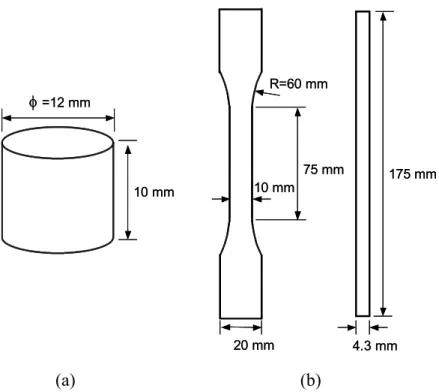
(20) Chapter 2 Polymer Modeling Since material properties of the polymer, i.e. Young’s Modules, Poisson’s ratio, and viscoplastic behavior, are required for modeling the behaviors of composites, tensile and compression tests were performed to determine the corresponding properties. The tensile test was performed to determine the Poisson’s ratio of the polymer while the compression test was employed to determine the Young’s modulus and the viscoplastic behavior of the polymer.. Based on the experimental data of. compression test at 10-4, 10-2, 1/s strain rates, the model coefficients of three parameters model [8] were determined and this model was applied to predict the Split Hopkinson Pressure Bar (SHPB) results up to 650/s strain rate.. Besides, the. coefficient of thermal expansion (CTE) of the polymer was measured to investigate the thermal stress effects on the off-axis composites.. 2.1 Experiments 2.1.1 Compression Test The polymer (Bisphenol A) in the form of powder provided from Ad-group Taiwan was filled into a pre-designed stainless mold for fabricating the cylindrical specimens.. In the beginning, the mold was putted into a vacuum oven and heated. from room temperature to 75 o C within 50 minutes.. During this process, the. polymer was changed from powder state to liquid state with very high viscosity and its volume decreased due to gas disappearance, then, some powder was replenished until the desired amount of polymer was reached.. In the next 8 minutes, the. temperature was raised to 95 o C and then kept for 130 minutes. the polymer was also degassing in the vacuum oven.. At the same time,. After degassing for a period of. time, the polymer was overflowed on the mold easily and we should open the door of the vacuum oven and scrape the polymer to retreat to cavities by using a thin plate. 7.
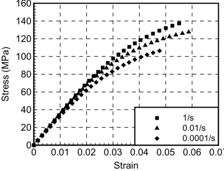
(21) It was to be noted that this scraping process must be finished as soon as possible (within 5 minutes) to avoid a large drop of oven temperature.. After repeating the. degassing and scraping process 6 times within the 130 minute, the temperature was held on 90 o C for 30 minutes to perform the curing process and raised to 145 o C within 10 minutes and maintained 60 minutes to carry out the post curing process. After the curing and post-curing processes, the specimens were removed from the mold with care.. In order to have parallel and smooth loading surfaces, all specimens. were polished using a polishing machine with 25.0µ aluminum oxide powers.. After. polishing, the final dimensions for the specimens are 10 mm in height and 12mm in diameter as shown in Fig. 2.1(a).. To demonstrate the strain rate effect on the. polymer, compression tests were performed on the cylindrical specimens using hydraulic MTS machine at three different strain rates, 10-4, 10-2 and 1/s.. Back to. back strain gages were adhered on the specimens for the strain measurement during compression tests. tests.. Fig. 2.2 demonstrates the experimental setup for the compression. The stress history was obtained from the load cell and the associated strain. history was measured from the strain gages mounted on the specimens.. During the. tests, both stress and strain signals were recorded by LabView together with PC computer.. All results of compression test were shown in Fig. 2.3 and the Young’s. modulus of the polymer was determined as 3.4 GPa.. 2.1.2 Tensile Test For measuring the Poisson’s ratio of the polymer, tensile tests were carried out on the coupon specimens, with the dimensions as shown in Fig. 2.1(b), fabricated in the same manner as described early excepted that the designed mode is different. Two strain gages were mounted on the centers of the specimens.. One was in the. axial direction and the other was in the lateral direction to measure the axial and 8.
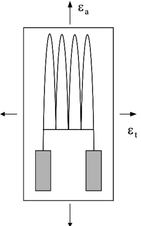
(22) transverse strains, respectively. The tensile test was implemented on a hydraulic MTS system at 10-4/s strain rate and the result was shown in Fig. 2.4. According to this result, the Poisson’s ratio of the polymer was evaluated as 0.37.. 2.1.3 Measurement of Coefficient of Thermal Expansion In the analysis of thermal residual stress effect, the coefficient of thermal expansion (CTE) of the matrix was measured first.. A simple method [25-27] has. been applied to finish this measurement in which the EA-06-062TT-120 strain gage was chosen and the adhesive M-bond 610 was used for its high operation temperature. The EA-06-062TT-120 strain gage has two pieces of electrical resistance on a unit, one is an axial field and the other is transverse.. Therefore, axial and transverse. deformations of a specimen can be measured at the same time.. Based on the strain. gage technique, when the gage was subjected to a biaxial strain field, as shown in Fig. 2.5, the following relation was found ∆R = Fa ε a + Ft ε t R. (2.1.1). where R = original gage resistance Fa = axial gage factor Ft = transverse gage factor ε a = axial strain field ε t = transverse strain field Define the transverse sensitivity coefficient K as K=. Ft Fa. (2.1.2). If the strain gage was mounted on a specimen with Poisson’s ratio ν 0 and the specimen was under a uniaxial loading, the strain fields can be represented as 9.
(23) ε t = −ν 0ε a. (2.1.3). Substituting eqns (2.1.2) and (2.1.3) into eqn (2.1.1) yields ∆R = Fa (1 − ν 0 K ) ε a = Fg ε a R. (2.1.4). where Fg = Fa (1 − ν 0 K ) is the well-known gage factor and the measured strain can be represented as εa =. ∆R R Fg. (2.1.5). Since eqn (2.1.4) can be applied only if the specimen was subjected to a uniaxial stress field and the transverse strain field was due to the Poisson’s ratio effect only, on the measurement of CTE, the matrix under thermal expansion was within a biaxial strain field and eqn (2.1.4) can not be followed directly. Therefore, the transverse sensitivity must be embraced to correct the gage results.. With the. assistance of measured strains at the axial and transverse direction, ε mx and ε my , the corrected strains ε x and ε y are given by [25] εx = εy =. (1 − ν 0 K ) (ε mx − Kε my ) 1− K2 (1 − ν 0 K ) (ε my − Kε mx ) 1− K2. (2.1.6) (2.1.7). It can be shown that in the current analysis, the strain of isotropic test material with Poisson’s ratio equal to 0.37 under the same measured strain ε mx = ε my will be about 2 % error if the correction equations (2.1.6) and (2.1.7) are not applied. It’s a slight effect so the correction hasn’t been done here. It was noted that when the gage was mounted on a stress free specimen and underwent temperature change, we can not say the gage signal was fully induced by the specimen deformation but also affected by the thermal effect.. To cancel the. thermal effect on the electrical resistance, a half-bridge circuit as shown in Fig. 2.6 10.
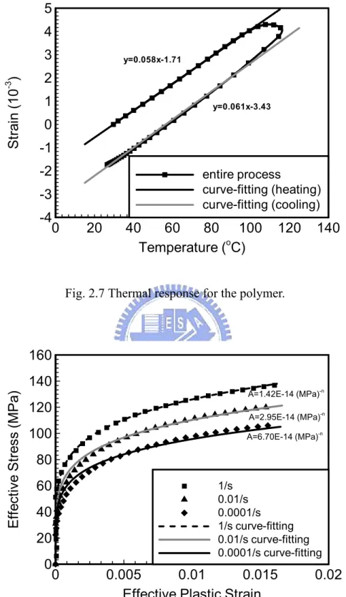
(24) was applied [26].. There are two materials in the system, one is the test material and. the other is the reference material. The CTE of the test material is unknown but known for the reference material.. Since αx − αr =. εx − εr ∆T. (2.1.8). and ∆E = V. R1R 2 ∆R1 ∆R 2 ∆R 3 ∆R 4 − + − (R1 + R 2 )2 R1 R 2 R 3 R 4 . (2.1.9). where α x is the CTE of the test material at measured direction, α r is the CTE of the reference material, ε x is the thermal strain from the test material and ε r is the thermal strain from the reference material.. By means of eqns (2.1.8) and (2.1.9), the. thermal effect on the electrical resistance can be eliminated skillfully and the CTE of the test material can be determined. The experimental system was placed in a programmable-control vacuum oven where the test material is a 30 × 20 × 2 mm3 thin plate and the reference material is a titanium silicate material with very small CTE (here we assume it is equal to zero). A thermal couple was adhered on the reference material to record the history of temperature change but not on the test material due to the limitation of specimen size. Because of low heating and cooling rate (about 19 0C/hr and 22 0C/hr, respectively), it can be assumed that the test and reference material possess the same temperature during heating and cooling processes so the temperature signal of the reference material can present the temperature of the test material, too. According to the final result shown in Fig. 2.7, the CTE of the matrix is about 5.9 × 10 −5 / o C from the average of heating and cooling slopes.. 11.
(25) 2.2 Visco-Plasticity Model A viscoplasticity model can be derived based on the low strain rate compression tests to describe the nonlinear rate dependent behavior of the epoxy materials. The epoxy material was treated as an isotropic von Mises plastic material and the J2 plastic potential. J2 =. [. ]. 1 (σ11 − σ22 ) 2 + (σ22 − σ33 ) 2 + (σ33 − σ11 ) 2 + σ122 + σ223 + σ132 6. was employed to develop the viscoplasticity model.. (2.2.1). By using the associated flow. rule, the plastic strain rate is expressed as ∂J ε& ijp = λ& 2 ∂σij. (2.2.2). where λ& is a proportional factor. Defining an effective stress σ as σ = 3J 2. (2.2.3). through the plastic work rate relation, i.e. & p = σ ε& p = σ ε& p = 2J λ& W ij ij 2. (2.2.4). the effective plastic strain rate ε& p can be expressed explicitly as. (. 2 1 p ε& = ε&11 − ε& p22 3 2 p. ) +( 2. ε& p22. ) +(. p 2 − ε& 33. p ε& 33. ). and the proportional factor λ& in eqn (2.2.2) was derived as. 12. 12. 3 p2 p2 p 2 + γ& 12 + γ& 23 + γ& 13 4. p 2 − ε&11 . (2.2.5).
(26) 3 ε& p 3 σ& λ& = = 2 σ 2 Hpσ. (2.2.6). where Hp. Hp =. σ& ε& p. (2.2.7). is the rate dependent plastic modulus. It is noted that for the J2 material subjected to uniaxial loading, the effective stress is equal to the axial stress and the effective plastic strain is the same as the axial plastic strain ε px obtained by subtracting the elastic part from the total measured strain ε x .. As a result, the effective stress and effective plastic strain curves of the. epoxy can be obtained directly from the experimentally determined axial stress and axial plastic strain curves. Fig. 2.8 shows the effective stress and effective plastic strain curves measured at strain rates of 10-4, 10-2 and 1/s. Let the effective stress – effective plastic strain curves could be fitted individually by a power law as ε p = A( σ ) n. (2.2.8). and the results were also illustrated in Fig. 2.8. It was found that the power index n in eqn (2.2.8) is constant for all strain rates. However, the amplitude A is a function of strain rate.. Again, assume that the amplitude A is a power law function of. effective plastic strain rate as [8]. ( ). A = χ ε& p. m. (2.2.9). Then a viscoplasticity model can be expressed in the form. ( ). ε p = χ ε& p 13. m. (σ )n. (2.2.10).
(27) It is noted that the effective stress and effective plastic strain curves plotted in Fig. 2.8 were produced for respective constant strain rates but not for constant effective plastic strain rates as required in the viscoplasticity model.. By subtracting. the elastic component from the total strain, the plastic strain component, and thus the effective plastic strain, can be obtained.. Fig. 2.9 shows the effective plastic. strain-time curves for epoxy specimens corresponding to strain rate of 10-4/s.. It is. evident from Fig. 2.9 that the effective plastic strain rate is not constant over the entire loading range.. Nevertheless, it almost reaches a constant value beyond ε p = 0.25% .. Since the initial deformation of the stress-strain curve is mainly dominated by the elastic response, in determining parameters χ and m in eqn (2.2.9), the data corresponding to the initial portion for which the effective plastic strain is less than 0.25% was truncated. Fig. 2.10 shows amplitude A as a function of effective plastic strain rate on the log-log scale for the epoxy material obtained from the compression tests.. The parameters χ and m are then determined from these plots as the. intercept and the slope, respectively. Once m and χ are determined, this model can be extrapolated to predict the material behavior at any strain rates. The values of the parameters in the viscoplasticity model for epoxy are listed in Table 1. With eqn (2.2.10), the rate dependent plastic modulus is expressed as. Hp =. 1 nχ( ε& ) ( σ ) n −1 p m. (2.2.11). According to the definition of the effective stress given in eqn (2.2.3), σ& was derived as 1 (2σ11 − σ22 − σ33 ) σ& 11 + (− σ11 + 2σ22 − σ33 ) σ& 22 + (− σ11 − σ22 + 2σ33 ) σ& 33 σ& = 2σ + 6σ 23σ& 23 + 6σ13σ& 13 + 6σ12σ& 12. (2.2.12). By substituting eqn (2.2.12) together with eqn (2.2.6) into eqn (2.2.2), the plastic strain rate is written as 14.
(28) p ε&11 p ε& 22 p ε& 33 9 1 p = 2 γ& 23 4 H p σ γ& p 13 p γ& 12 . S12 . S1S2. S1S3. S22. S1S4. S1S5. S2S3 S2S4 S2S5 S32. S3S4 S24. symmetric. S3S5 S4S5 S52. S1S6 σ& 11 S2S6 σ& 22 S3S6 σ& 33 S4S6 σ& 23 S5S6 σ& 13 S62 σ& 12 . (2.2.13). where 1 (2σ11 − σ 22 − σ33 ) 3 1 S2 = (− σ11 + 2σ 22 − σ 33 ) 3 1 S3 = (− σ11 − σ 22 + 2σ 33 ) 3 S4 = 2σ 23 S1 =. (2.2.14). S5 = 2σ13 S6 = 2σ12. In combination of the elastic parts, the constitutive relation of epoxy material at various strain rates was established as. { ε& } = [ SM ]{ σ& }. (2.2.15). [ S ] = [ S ]+ [ S ]. (2.2.16). where M. In eqn (2.2.16), and. [S ] p. e. p. [ S ] represents the elastic compliance matrix of the epoxy e. denotes the plastic compliance matrix given in eqn (2.2.13).. It is to be. noted that with eqn (2.2.15), the epoxy material properties at different loading rates could be characterized from which, through a micromechanical analysis, the mechanical behaviors of polymeric composites could also be generated. Inverting eqn (2.2.15), we derived 15.
(29) { σ& } = [ C M ]{ ε& }. (2.2.17). [ C ]= [S ]. (2.2.18). where M. M −1. The constitutive relation expressed in the form of eqn (2.2.17) was used in chapter 4 as the matrix material properties for the generalized method of cells micromechanical model.. 2.3 Modeling of Split Hopkinson Pressure Bar Results The stress and strain relations of polymer (Bisphenol A) under high strain rate were found using the steel SHPB apparatus. The gas pressure of 100 psi was used to push the steel striker bar and the compression wave was generated in the steel incident bar with 3 mm thickness copper pulse shaper attached on the impact surface.. The. compression wave signals were obtained by a pair of diametrically opposite gages mounted on the middle of the incident bar and the transmission bar.. The. amplification factors of incident bar channel and transmission bar channel were both set at 400. The excitation voltages of the Wheatstone bridge circuits were set at 5V. However, the amplification factor of specimen gage signal was set at 25 and excitation voltage was set at 3V. The sampling rate of oscilloscope was set at 10 MHz to record the voltage signals from Wheatstone bridge circuits and the final stress - strain curve of the polymer was shown in Fig. 2.11 where the Young’s modulus was determined as 3.9 GPa.. With the assistance of given stress history from experiments. as shown in Fig. 2.12, the associated plastic strain rates can be estimated by eqn (2.2.13) in which the effective stress was evaluated using eqn (2.2.3) and the effective. 16.
(30) plastic strain rate embedded in the plastic modulus H p was determined through eqn (2.2.5). Then, the total strain was constructed through the combination of elastic strains and plastic strains. The prediction result was plotted together with MTS results and shown in Fig. 2.13.. Since the Young’s modulus of the polymer up to. 650/s strain rate attains to 3.9 GPa greater than the MTS result 3.4 GPa, the polymer somehow exists viscoelastic behavior but wasn’t considered in the three parameters model.. Therefore, there is a significant distinction between the prediction and. experimental results due to the effect of different elastic strain.. 17.
(31) Chapter 3. Square Fiber Model. In this chapter, the square fiber model (SFM) proposed by Sun and Chen [12] for modeling the composite nonlinearity was reviewed. Since the typical square fiber model was constructed based on the square edge packing array as shown in Fig. 3.1(a), it can not be applied to other fiber arrangements, like the square diagonal packing array demonstrated in Fig. 3.1(b).. As a result, a modified SFM was. developed to account for the RVE with various fiber arrangements.. In addition, the. thermal stress effect was considered using SFM and will be discussed in chapter 6.. 3.1 Square Fiber Model Sun and Chen [12] proposed a representative volume element (RVE) as shown in Fig. 3.2 for unidirectional composites.. This RVE is so-called square edge packing. array (SEP) as shown in Fig. 3.1(a). In this RVE, the round fiber is approximated by a square one with a cross-section area equal to that of the circular one.. It is noted. that because of geometric symmetry, only a quarter of the RVE is considered.. This. RVE is composed of three subregions, AF, AM and B, in which AF stands for the fiber; AM and B stand for the matrix. Region A.. Subregions AF and AM were assembled into. The fiber subregion AF is considered to be a square cross-section with. the same cross section area of the original quarter circle. The coordinate system is set up such that the fiber direction is parallel to the x1 axis.. A plane stress. assumption prevails in the x1 − x 2 plane such that the out of plane stress components would vanish ( σ13 = σ 23 = σ33 = 0 ).. In addition, the follow assumptions are also. made. (a) The stress and strain states are uniform in all subregions. (b) In region A, the stress and strain fields in AF and AM follow suitable constant stress or constant strain assumptions, i.e. 18.
(32) AF AM A σ12 = σ12 = σ12 (constant stress) AM A σAF 22 = σ 22 = σ 22 (constant stress) AF AM A ε11 = ε11 = ε11. (3.1.1). (constant strain). (c) For combination of region A and B, the constant strain assumptions are made, i.e.. A B ε11 = ε11 = ε11. ε A22 = ε B22 = ε 22. (3.1.2). A B γ12 = γ12 = γ12. Based on the micromechanics, the average stress and strain fields in the subregion A are treated as σijA =. 1 AF + AM. εijA =. 1 AF + AM. (∫. (∫. AF. σijAFdA + ∫. ε AFdA + AF ij. AM. σijAM dA. ∫ AM εij. AM. dA. ). ). (3.1.3). (3.1.4). , and the average stress and strain fields in the RVE are given by σij =. 1 A+B. (∫. εij =. 1 A+B. (∫. A. σijA dA + ∫ σijBdA B. ε A dA + A ij. ). ∫ B εij dA ) B. (3.1.5) (3.1.6). The explicit forms for eqns (3.1.3)-(3.1.6) expressed in terms of local stress and strain with the assistance of eqns (3.1.1) and (3.1.2) are derived as A AF AM σ11 = v1σ11 + v 2σ11 AM ε A22 = v1ε AF 22 + v 2 ε 22 A γ12. =. AF v1γ12. +. (3.1.7). AM v 2 γ12. and A B σ11 = v A σ11 + v Bσ11. σ 22 = v A σ A22 + v Bσ B22 A B σ12 = v A σ12 + v Bσ12. where 19. (3.1.8).
(33) v1 =. h1 h1 + h 2. v2 =. h2 h1 + h 2. vA =. h3 h3 + h 4. vB =. h4 h3 + h 4. (3.1.9). It is noted that v1 and v 2 , represent the volume fraction of subregions AF and AM with respective to the region A, and v A and v B indicate the volume fraction of regions, A, B, respectively to the RVE.. With eqns (3.1.1), (3.1.2), (3.1.7). and (3.1.8), the relationships between the subregion stresses and strains and the RVE stresses and strains were established.. To derive the stress and strain relations of the. RVE, the corresponding fiber and matrix properties must be given in advance.. The. fiber is considered to be an orthotropic elastic material. Therefore, in the region AF, we have the incremental stress and strain relations. { dε }= [ S ]{ dσ } AF. AF. 1 F E1 − νF = F12 E1 0 . − ν F21 E F2 1 E F2. AF. (3.1.10). where. [S ] AF. 0. 0 0 1 F G12 . (3.1.11). While, the matrix phase is considered to be an elastic-plastic material and can be characterized by the plasticity model mentioned in chapter 2.. Since the square. fiber model is a 2-D plane stress model, the 2-D von Mises J2 is given as. (. 1 AM J 2 = σ11 3 . ) + (σ ) 2. AM 2 22. (. ). AM AM AM 2 − σ11 σ 22 + 3 σ12 . (3.1.12). Substituting J2 into flow rule and following the same derivatives in chapter 2 with the assistance of power law relation given in eqn (2.2.8) leads to. { dε }= [ S ]{ dσ } AM. AM. AM. (3.1.13). which gives a relation between total strain increment and stress increment for all pure matrix regions, i.e. AM and B, and the components of compliance matrix 20. [S ] AM. in.
(34) eqn (3.1.13) were. (. AM S12 AM S16. SAM 22 SAM 26 AM S66. ). 1 9 AM n − 3 AM AM An S1 S1 + σ EM 4 n − 3 AM AM νM 9 S1 S2 = SAM = − + An σ AM 21 M 4 E n − 3 AM AM 9 AM S1 S3 = S61 = An σ AM 2 n − 3 AM AM 1 9 S 2 S2 = M + An σ AM 4 E n − 3 AM AM 9 AM S2 S3 = S62 = An σ AM 2 n − 3 AM AM 1 = M + 9An σ AM S3 S3 G. AM S11 =. (. (. ). (. ). (. ). (. ). (3.1.14). ). in which S1AM =. (. ). SAM 2. (. ). S3AM. 1 AM 2σ11 − σ AM 22 3 1 AM = 2σ AM 22 − σ11 3 AM = σ12. (3.1.15). With the stresses and strains relations for subregions AF and AM (given in eqn (3.1.10) and eqn (3.1.13), respectively), the constitutive relation of subregion A was generated through eqns (3.1.1) and (3.1.7) and the explicit results are given by A A A A A dσ11 S11 dε11 S12 S13 A A A A A dε 22 = S21 S22 S23 dσ 22 dγ A SA SA SA dσ A 62 66 12 12 61. (3.1.16). where A = a1 E1F S11 A F = SA21 = a 2 E1F − ν12 S12 E1F A A = S61 = a 3 E1F S16. (. ). (. F AM SA22 = v1 1 E F2 − ν12 a 2 E1F + v 2 b 2SAM 21 + S22. (. A F AM = − v1a 3 ν12 SA26 = S62 E1F + v 2 b3SAM 21 + S26. (. A F AM AM = v1 G12 + v 2 b3S61 + S66 S66. in which 21. ). ). ). (3.1.17).
(35) a1 = (1 − v 2b1 ) v1 a 2 = − v 2 b 2 v1 a 3 = − v 2 b3 v1. (. AM + v2 b1 = v1E1FS11. (. ). (3.1.18). −1. )(. AM F AM + ν12 + v2 b 2 = − v1 E1FS12 v1E1FS11. (. AM AM + v2 b3 = − v1E1FS16 v1E1FS11. ). ). −1. −1. Inverting eqn (3.1.16), we obtain. { dσ }= [ C ]{ dε }. (3.1.19). [ C ]= [S ]. (3.1.20). A. A. A. where A −1. A. For the region B, since it is matrix materials, the compliance matrix is exactly the same as that in eqn (3.1.13).. Thus, the incremental stresses and strain relation is. expressed as. { dε }= [ S ]{ dσ } B. , and. B. B. (3.1.21). [ S ] is the same as [ S ]. B. AM. Inverting eqn (3.1.21), we obtain. { dσ }= [ C ]{ dε }. (3.1.22). [ C ]= [S ]. (3.1.23). B. B. B. where B −1. B. Again, with constitutive relation of region A and B (given by (3.1.19), and (3.1.21)), through eqn (3.1.8) and eqns (3.1.2), the incremental stress and strain relation of entire RVE was derived as. { dσ } = [ C ]{ dε }. (3.1.24). where. [C] = v A [ CA ]+ v B [ CB ] 22. (3.1.25).
(36) With eqn (3.1.24), for a given loading history, the constitutive relation of the composites can be generated by using the numerical iteration. At the beginning, the overall stiffness matrix [C] of composites in eqn (3.1.24) was constructed with initial stress states equal to zero. For a tiny stress increment, the corresponding strain increment was calculated from eqn (3.1.24). The strain increments in RVE are exactly the same as those in regions A and B based on the constant strain assumption given in eqn (3.1.2), and the corresponding stress increments in the two regions were evaluated with the assistance of the respective constitutive law given in eqns (3.1.19) and (3.1.22).. Since region B was pure matrix, its stress components was directly. substituted into eqn (3.1.14) to update the stiffness matrix. [ C ]. B. However, for. region A, there are two subregions, AM and AF enclosed. In order to update the stiffness matrix. [ C ], A. the stress components in the subregion AM need to be. evaluated, since the compliance matrix. [S ] AM. in eqn (3.1.13) is dependent on the. AM stress states. The incremental stress states dσ AM and dσ12 in the subregion AM 22 A can be evaluated directly from dσ A22 and dσ12 in the region A based on the constant. stress assumption.. AM Similarly, the incremental strain sate dε11 was also obtained. A with constant strain assumption. from dε11. Once the stress components dσ AM and 22. AM AM AM dσ12 and the strain component dε11 were determined, the stress increment dσ11. could be derived through the first relation of eqn (3.1.13).. With the stress. components in the subregion AM, the corresponding compliance. [S ]. eqn (3.1.13) was renewed. an updated stiffness matrix. By combining the compliance. [S ] AF. AM. matrix in. of subregion AF,. [ C ] was obtained and thereafter, the new stiffness A. [C]. of the RVE was calculated which was employed to evaluate the strain increment in the next step associated with other tiny stress increments. 23. The detail program for the.
(37) SFM combined with three parameters model was attached in the Appendix A.. 3.2 Modified Square Fiber Model Since the square fiber model (SFM) proposed by Sun and Chen [12] was derived based on the square edge packing with a square fiber inside, it is difficult to deal with the RVE with circular fiber together with different fiber arrangements by using the SFM.. To overcome this problem, a modified SFM was proposed in this. section by dividing the representative volume element (RVE) into numbers of horizontal tiny subcells.. The constant stress (or constant strain) conditions applied. in the SFM (shown in the previous section) were again employed at each subcells in the modified SFM.. There are two fiber arrangements considered here, i.e. square. edge packing array and square diagonal packing array, which were illustrated respectively in Fig. 3.1(a) and Fig. 3.1(b).. 3.2.1 Square Edge Packing Array In the case of square edge packing array as shown in Fig. 3.3, the RVE consists of a region A with a height h f equal to the radius r of the fiber and a pure matrix region B with a height of h m which is equal to l − r . length of the square RVE.. It is noted that l is the. There are two subregions AF and AM contained in the. region A. The region A was divided into N subcells horizontally from A1 to An and the height of each subcell is h f N .. Thus, in each subregion An consisting of AFn. and AMn, the stress and strain fields follow constant stress or constant strain assumptions, i.e. AFn AMn An σ12 = σ12 = σ12 AMn n σ AF = σ A22n 22 = σ 22. ε. AFn 11. =ε. AMn 11. =ε. An 11. 24. n = 1,2,3,..., N. (3.2.1).
(38) On the other hand, for the RVE, the following assumptions were applied, AN A1 A2 B ε11 = ε11 = L = ε11 = ε11 = ε11. ε A221 = ε A222 = L = ε A22N = ε B22 = ε 22. (3.2.2). AN A1 A2 B γ12 = γ12 = L = γ12 = γ12 = γ12. Based on the micromechanics, the average stress and strain fields for each subcell An are defined as σijA n =. 1 AFn + AM n . ∫ AF σij. dA + ∫. εijA n =. 1 AFn + AM n . ∫ AF εij. dA + ∫. AFn. n. AFn. n. σijAM n dA . (3.2.3). εijAM n dA . (3.2.4). AM n. AM n. and, for the RVE, they are given by σij =. N B dA σ + ∑ ∫ A n σijA n dA N ∫ B ij n =1 B + ∑ An . 1. (3.2.5). n =1. εij =. N B dA ε + ε A n dA ∑ ij N ∫ ∫B A n ij n =1 B + ∑ An . 1. (3.2.6). n =1. Substituting eqns (3.2.1) and (3.2.2) into eqns (3.2.3)-(3.2.6) yields AMn AFn An σ11 = v AFn σ11 + v AMn σ11 AM n AM n n ε A22n = v AFn ε AF ε 22 22 + v. n = 1,2,3,...N. (3.2.7). AMn AFn An γ12 = v AFn γ12 + v AMn γ12. and N. (. ). (. ). (. ). An B σ11 = ∑ v A n σ11 + v Bσ11 n =1 N. σ 22 = ∑ v A n σ A22n + v Bσ B22 n =1 N. (3.2.8). An B σ12 = ∑ v A n σ12 + v Bσ12 n =1. where v AFn and v AM n represent the volume fraction of fiber and matrix phases with respect to the subcell An, and v A n and v B denote the volume fraction of subregion An and subregion B with respect to entire RVE, respectively. Based on geometric correlation given in Fig. 3.2, the volume fractions, v A n and v B can be 25.
(39) determined directly as v An =. hf N hf + hm. (3.2.9). hm v = hf + hm B. However, in order to evaluate the volume fraction, v AFn and v AM n in the subcell An with convenience, the angle θn was defined as the orientation of the ray emanating from the fiber center to the intersection of the fiber circumference and the nth horizontal grid line.. Thus, the corresponding volume fraction is written as v AFn =. r cos θ n l. v AMn = 1 − v AFn. (3.2.10). where θn = sin −1. (n − 1) h f rN. n = 1,2,3,..., N. (3.2.11). can be determined from the geometric correlation given in Fig. 3.2.. For the. sub-region An, it has the same constitutive relation as shown in eqn (3.1.16) except that the volume fractions v1 and v 2 are replaced by v AFn and v AM n , respectively, and also that in the sub-cell AMn, the compliance matrix becomes. [ S ]. AM. [S ] AM n. instead of. Therefore, the constitutive equation for subcell An is expressed as An An dε11 S11 An An dε 22 = S21 dγ A n SA n 12 61. An S12 SA22n An S62. where. 26. An An dσ11 S13 SA23n dσ A22n An An S66 dσ12 . (3.2.12).
(40) An = a1 E1F S11 An F = SA21n = a 2 E1F − ν12 S12 E1F An An = S61 = a 3 E1F S16. (. ). ( (b S +v ) +S. F n n + SAM SA22n = v AFn 1 E F2 − ν12 a 2 E1F + v AM n b 2SAM 21 22 AM n. An F SA26n = S62 E1F = − v AFn a 3 ν12. (. An AM n F S66 = v AFn G12 + v AM n b3S61. AM n 3 21. n + SAM 26. ) ). (3.2.13). AM n 66. in which. (. ). a1 = 1 − v AM n b1 v AFn a 2 = − v AM n b 2 v AFn a 3 = − v AM n b3 v AFn. (. AM n b1 = v AFn E1FS11 + v AM n. (. AM n F b 2 = − v AFn E1FS12 + ν12. (. ) )(v. (3.2.14). −1 AFn. AM n E1FS11 + v AM n. AM n AM n b 3 = − v AFn E1FS16 v AFn E1FS11 + v AM n. where. [S ] An. ). [S ] AM n. −1. −1. is the compliance matrix of subcell An.. mathematical form of compliance matrix. ). It is to be noted that the. is the same as that in eqn (3.1.13),. which was evaluated in terms of the current stress states of subcell AMn. Again, for the region B, the constitutive equation is the same as eqn (3.1.21) which was rewritten as. { dε }= [ S ]{ dσ } B. B. B. (3.2.15). With ingredient constitutive equations given in eqns (3.2.12) and (3.2.15) together with eqns (3.2.2), (3.2.8), we derived the incremental form of overall constitutive equation as. { dσ } = [ C ]{ dε }. (3.2.16). where. [ C ] + v [ C ]+ L + v [ C ]+ v [ C ] = ∑ v [ C ]+v [ C ]. [C] = v A. 1. N. A1. An. A2. An. A2. B. B. n =1. 27. AN. AN. B. B. (3.2.17).
(41) 3.2.2 Square Diagonal Packing Array In addition to the square edge packing array for the fiber arrangement, there are other fiber arrangements called the square diagonal packing (SDP) array which will be discussed in this section. Fig. 3.1(b) shows the typical RVE for this fiber arrangement.. Because of symmetry, only one quarter of the RVE will be considered. in the analysis.. In fact, due to different fiber fractions, there are three possible. situations to be accounted for the generation of the constitutive relations as shown in Fig 3.4. It was found that the critical fiber volume fraction for SDP is 39.3 %. Above this value, two quarter fibers will have interaction within the center region of the RVE as shown in Fig. 3.4(c). It was noted that Fig. 3.4(d) shows the maximum fiber volume fraction of SDP is 78.5 %.. Since, in industrial applications of fiber. composites, the fiber volume fraction is around 60% which is greater than the critical value, and thus we only consider the case with higher volume fractions.. As shown. in Fig. 3.5, the RVE was separated into three partitions initially with two horizontal lines.. One was along the top of the left fiber and the other was passing through the. bottom of the right fiber. Let us denote the center region as subregion B with a height of h B which is equal to 2r − l , and the other two regions as subregion A with the individual height , h A , equal to l − r , where l is the length of the square RVE and r is the radius of the fiber. Noted that there are two subregions, i.e., AF (fiber phase of region A) and AM (matrix phase of region A) contained in the region A, and three subregions, i.e., BFL (fiber phase in the left side of region B), BM (matrix phase of region B) and BFR (fiber phase in the right side of region B), were included in the region B. Subsequently, regions A and B were divided into N and M horizontal subcells, represented by An and Bn respectively, such that totally there are 2N+M subcells enclosed in the RVE.. The height for each subcell An in region A is h A N ,. while for subcell Bn in region B, the height is h B M . 28. In order to determine the.
數據
+7
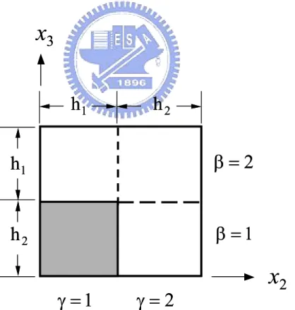
![Fig. 4.1 The coordinate system and geometry information of the generalized method of cells [15]](https://thumb-ap.123doks.com/thumbv2/9libinfo/8116868.165756/102.892.242.641.125.492/fig-coordinate-geometry-information-generalized-method-cells.webp)
相關文件
Wang, Solving pseudomonotone variational inequalities and pseudocon- vex optimization problems using the projection neural network, IEEE Transactions on Neural Networks 17
Define instead the imaginary.. potential, magnetic field, lattice…) Dirac-BdG Hamiltonian:. with small, and matrix
incapable to extract any quantities from QCD, nor to tackle the most interesting physics, namely, the spontaneously chiral symmetry breaking and the color confinement..
Indeed, in our example the positive effect from higher term structure of credit default swap spreads on the mean numbers of defaults can be offset by a negative effect from
Microphone and 600 ohm line conduits shall be mechanically and electrically connected to receptacle boxes and electrically grounded to the audio system ground point.. Lines in
When ready to eat a bite of your bread, place the spoon on the When ready to eat a bite of your bread, place the spoon on the under plate, then use the same hand to take the
Jin-Jei Wu, Daru Chen, Kun-Lin Liao, Tzong-Jer Yang, and Linfang Shen, “A novel fiber sensor based on a Bragg fiber with a defect layer”, Presented in 2009 Annular Meeting of
The fist type of photonic crystal fiber is composed of a solid silica core with modulation core refractive index and a cladding with triangular lattice elliptical air holes,
