以反透視映射模型與移動補償為基礎的障礙物偵測應用在倒車行為的安全上

i

國

立

交

通

大

學

生醫工程研究所

碩

士

論

文

以反透視映射模型與移動補償為基礎的障礙物

偵測應用在倒車行為的安全上

Generic Obstacle Detection for Backing-Up Maneuver Safety

Based on Inverse Perspective Mapping and Movement

Compensation

研 究 生：李嶸健

指導教授：林進燈 教授

ii

以反透視映射模型與移動補償為基礎的障礙物偵測應用在倒車行為

的安全上

Generic Obstacle Detection for Backing-Up Maneuver Safety Based on

Inverse Perspective Mapping and Movement Compensation

研 究 生：李嶸健 Student：Jung-Chien Lee

指導教授：林進燈 Advisor：Chin-Teng Lin

國 立 交 通 大 學

生 醫 工 程 研 究 所

碩 士 論 文

A Thesis

Submitted to Institute of Biomedical Engineering College of Computer Science

National Chiao Tung University in partial Fulfillment of the Requirements

for the Degree of Master

in

Computer Science

July 2010

Hsinchu, Taiwan, Republic of China

iii

以反透視映射模型與移動補償為基礎的障礙物

偵測應用在倒車行為的安全上

學生：李嶸健

指導教授：林進燈 博士

國立交通大學生醫工程研究所

摘要

近年來，交通事故造成人員受傷或死亡的數量仍然居高不下，因此世界各地 提升安全性的高效能車輛與日俱增，其中車輛與其他障礙物碰撞事故發生最為頻 繁，很多研究人員提出利用立體視覺的一般障礙物偵測技術，然而，影像式駕駛 輔助安全系統中在移動車輛中以單支攝影機的障礙物偵測仍然是一個困難且具 有挑戰性的問題。在本篇論文中，我們提出一個以移動補償與反透視映射模型為 基礎的單眼影像式障礙物偵測技術，提出一個創新的地面移動量估測技術藉由利 用路面偵測取得影像中最有用的地面特徵點，並且分析特徵點的光流主要分布， 可以準確的獲得地面移動補償量，此外，利用反透視映射模型對影像中平面與非 平面物體的不同特性來偵測障礙物。為了要得到更可靠的偵測結果與最靠近的可 能碰撞位置，一個垂直方向的統計將被用來定位物體。我們提出的方法將會估計 目標物離本車的距離來做更進一步的安全應用，最後我們測試了很多在日常生活 倒車場景中可能會發生的情況，藉由實驗結果可證明我們提出的系統在障礙物偵 測與距離估測上可達到一定的穩健性與準確性。

iv

本論文的目標是希望藉由偵測阻礙行進路線上或突出地面具有一定高度的 物體來提升倒車行為的安全，此外，藉由標示目標物離本車最近的位置與距離， 可有效的避免在倒車上的碰撞。

v

Generic Obstacle Detection for Backing-Up

Maneuver Safety Based on Inverse Perspective

Mapping and Movement Compensation

Student: Jung-Chien Lee

Advisor: Dr. Chin-Teng Lin

Institute of Biomedical Engineering

College of Computer Science National Chiao Tung University

ABSTRACT

The number of road traffic accidents which involves the fatality and injury accidents is so much in recent years, so that the number of higher performance vehicles for safety is growing up over the world. Among of all the collision accidents between vehicle and other generalized obstacles occur most frequently. For generic obstacle detection, researchers have proposed many methods which focus on stereo vision. However, automatic obstacle detection with a single camera system mounted on a moving vehicle is still a challenging problem in vision-based safety driving support systems. In this paper, we present a monocular vision-based obstacle detection algorithm which is based on movement compensation and IPM. We proposed a novel ground movement estimation technique which is employing road detection to assist in obtaining most useful ground features in the image, and analysis the principal distribution of optical flow of these feature points, the ground movement for compensation is obtained accurately. Besides, adopting different characteristics

vi

between planar and non-planar object result from IPM to detect obstacle. In order to get more reliable detection and the nearest collision position, a vertical profile is used to locate the obstacle. Furthermore the proposed technique is to measure the distance of target how far away ego-vehicle for safety application. This system has been tested for many conditions which could occur when backing up in real life situations, and the experimental results already demonstrated the effectiveness and accurateness of the proposed obstacle detection and distance measurement technique.

The objective of this paper is to improve the safety for backing up maneuver by detecting objects that can obstruct the vehicle’s driving path or anything raise out significantly from the road surface. Besides, backing up collision can be avoided effectively by marking the nearest position and indicating the distance away from our ego-vehicle.

vii

致 謝

本論文的完成，首先要感謝指導教授林進燈博士這兩年來的悉心指導，不管 在學業或研究方法上都提供我許多意見與想法，這些寶貴的知識讓我受益良多。 另外也要感謝口試委員們的建議與指教使本論文更為完整。 其次，感謝超視覺實驗室的蒲鶴章博士與范剛維博士，還有建霆、子貴、肇 廷、Linda、東霖、勝智學長姐們，以豐富的知識與過來人的經驗給予我莫大的 幫助，同學佳芳、哲男、健豪、聖傑的相互砥礪共同奮鬥，這段日子有苦有笑， 我會懷念我們一起為實驗為論文奮戰的時光，還有學弟們在研究過程中的幫忙， 提供建議、拍攝影片、打氣鼓勵、製造歡樂，因為有你們在 915 的日子很快樂。 其中特別感謝子貴學長，在理論及程式技巧上給予我相當多的幫助與建議，讓我 獲益良多。還有感謝超視覺實驗室給我的一切，這兩年來不管是知識的學習還是 待人處事上讓我成長很多並且終身受用。 最後要感謝我最愛的父母，對我的教育與栽培，在我求學的路上總是不斷的 給予我鼓勵與關懷，一點一滴，永藏於心，並給予我精神及物質上的一切支援， 使我能安心地致力於學業。此外也感謝妹妹佳敏對我不斷的關心與支持。 謹以本論文獻給我的家人及所有關心我的師長朋友們。

viii

Contents

 

Chinese Abstract ... iii

English Abstract ... v

Chinese Acknowledgements ... vii

Contents ... viii List of Tables ... x List of Figures ... xi Chapter 1 Introduction... 1 1.1 Background   ... 1  1.2 Motivation   ... 3  1.3 Objective   ... 5  1.4 Thesis Organization   ... 5 

Chapter 2 Related Works ... 7

2.1 Related Works of Inverse Perspective Mapping (IPM) ... 7 

2.2 Related Works of Obstacle Detection  ... 8 

Chapter 3 System Overview and Fundamental Techniques ... 11

3.1 System Overview  ... 11 

3.2 Inverse Perspective Mapping (IPM) ... 13 

3.3 Optical Flow  ... 17 

Chapter 4 Obstacle Detection Algorithm ... 22

4.1 Feature Point Extraction  ... 22 

4.1.1 Feature Analysis ... 22

4.1.2 Road Detection ... 25

4.1.3 Feature Point Extraction ... 31

ix

4.2.1 Ground Motion Estimation ... 33

4.2.2 Compensated Image Building ... 37

4.2.3 Compensation Verification ... 39

4.3 Obstacle Localization   ... 41 

4.3.1 Obstacle Candidate Image ... 41

4.3.2 Obstacle Localization ... 42

4.4 Obstacle Verification  ... 45 

4.5 Distance Measurement  ... 46 

Chapter 5 Experimental Results ... 49

5.1 Experimental Environments  ... 49 

5.2 Experimental Results of Obstacle detection  ... 49 

5.3 Accuracy Evaluation   ... 54 

5.3.1 Compensation Evaluation ... 54

5.3.2 Accuracy Evaluation of Obstacle detection ... 56

5.3.3 Accuracy Evaluation of Obstacle Distance ... 58

Chapter 6 Conclusions and Future Work ... 59

x

List

of Tables

Table 1-1: The sub-items of intelligent transportation system ... 1

Table 1-2: Case number of traffic accidents over the world from 1997 to 2008 ... 4

Table 5-1 Comparison results of compensation error ... 55

Table 5-2 Accuracy evaluation of proposed obstacle detection ... 57

Table 5-3 Accuracy evaluation of [6] ... 57

xi

List of Figures

Fig. 3-1 System Flowchart ... 12

Fig. 3-2 System Flowchart ... 13

Fig. 3-3: The expectative results of diagrams (a) perspective effect removing (b) the property of a vertical straight line (c) the property of a horizontal straight line ... 15

Fig. 3-4: (a) Bird’s view and (b) side view of the geometric relation between world coordinate and image coordinate system ... 15

Fig. 3-5: Geometric relation of image coordinate system and world coordinate system ... 16

Fig. 3-6: Two-dimensional optical flow at a single pixel:optical flow at one pixel is underdetermined and so can yield at most motion, which is perpendicular to the line described by the flow equation ... 20

Fig. 4-1 Results of edge detection and its corresponding optical flow ... 24

Fig. 4-2 Results of corner detection and its corresponding optical flow ... 24

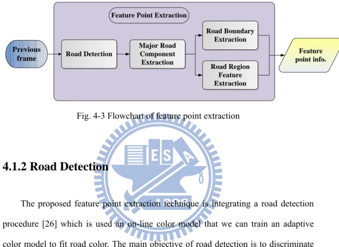
Fig. 4-3 Flowchart of feature point extraction ... 25

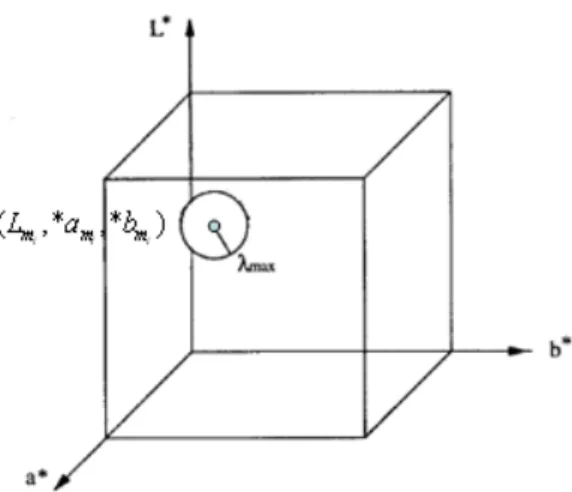
Fig. 4-4 A color ball i in the L*a*b* color model whose center is at (Lm, *am, *bm) and with radius λ ... 28 _max Fig. 4-5 Sampling area and color ball with a weight which represents the similarity to current road color ... 28

Fig. 4-6 Pixel matched with first B weight color balls which are the most represent standard color ... 30

Fig. 4-7 Results of road detection ... 31

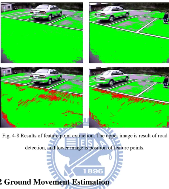
Fig. 4-8 Results of feature point extraction. The upper image is result of road detection, and lower image is position of feature points ... 32

Fig. 4-9 flow of ground movement estimation ... 33

Fig. 4-10 Difference between optical flow of original image and those of bird’s view image when vehicle is moving straight ... 34

Fig. 4-11 Difference between optical flow of original image and those of bird’s view image when vehicle is turning ... 35

xii

Fig. 4-12 Differences between optical flows of obstacle and those of planar object 35

Fig. 4-13 Histogram distribution of optical flow in world coordinate system ... 36

Fig. 4-14 Two-dimensional coordinate plane ... 37

Fig. 4-15 procedure of the compensated image building ... 39

Fig. 4-16 Chart of temporal coherence ... 40

Fig. 4-17 Flow of Obstacle Detection ... 41

Fig. 4-18 results of image difference between current image and compensated image ... 42

Fig. 4-19 Flowchart of obstacle localization ... 43

Fig. 4-20 the obstacle candidate image and the corresponding vertical-orientated histogram ... 44

Fig. 4-21 Procedure of creating vertical-orientated histogram ... 45

Fig. 4-22 procedure of obstacle verification ... 46

Fig. 4-23 Transformation between image coordinate and world coordinate ... 47

Fig. 4-24 Scale measure between world coordinate and real length ... 48

Fig. 4-25 flow of distance measurement ... 48

Fig. 5-1 Environment of camera setup ... 49

Fig. 5-2 Pedestrian stop on vehicle’s driving path ... 51

Fig. 5-3 Pedestrian crossing on vehicle’s driving path ... 51

Fig. 5-4 A typical parking situation ... 52

Fig. 5-5 Multiple objects in parking situation ... 53

Fig. 5-6 A low contrast environment when backing up ... 53

Fig. 5-7 A low contrast environment and interfered by brake lights when backing up ... 54

Fig. 5-8 Diagram of ground truth building ... 55

Fig. 5-9 Result of erroneous ground movement ... 57

1

Chapter 1.

Introduction

 

1.1 Background

The history of vehicle could be traced back to the 18th century. At that time, vehicle was a simple steam-powered three wheeler. As time goes on, there are many variations on vehicle improvement, such as the change of power, the change of style, and the change of function.

Nowadays, in addition to the consideration of vehicle style and brand, more and more consumers would take other factors into account. For example: the safety of vehicle, the entertainment equipments, the engine performance of vehicle and so on. Due to the demands of consumers, new generation vehicle which involves in the intelligent transportation system (ITS) has been developed rising and flourishing. The intelligent transportation system sub-items are listed in Table 1-1 [1].

Table 3-1: The sub-items of intelligent transportation system

Items Some sub-items

Advanced Traffic Management Systems (ATMS)

Changeable Message Sign Weigh-In-Motion

Electronic Toll Collection Automatic Vehicle Identification

Advanced Traveler Information Systems (ATIS)

Highway Advisory Radio Global Positioning System Wireless Communications Advanced Vehicle Control and Safety Systems

(AVCSS)

Collision Avoidance Systems Driver Assistance Systems Automatic Parking System Commercial Vehicle Operations Automatic Cargo Identification

2

(CVO) Automatic Vehicle Location

Advanced Public Transportation Systems (APTS)

Automatic Vehicle Monitoring

Electronic Fare Payment

The intelligent transportation system which we emphasize on advanced vehicle

can be subdivided into two parts: (1) high performance and pollution-less power (2) intelligent control and advanced safety. For high performance and pollution-less power, many engineers have developed some new fuels or power such as bio-alcohol, bio-diesel fuel, hydrogen-based power, and hybrid power. For intelligent control and advanced safety, the objective of this part is to assist drivers when they are inattentive by using sensors and controllers. There are great deals of researches that have been done in this part. For instance, pre-collision warning system, intelligent airbags, electronic stability program (ESP), adaptive cruise control (ACC), lane departure warning (LDW) and so on.

More and more international vehicle companies or groups have invested in driving safety applications, for example, Toyota, Honda, and Nissan in Japan developed many products continuously. In Europe, the PREVENT project of i2010 will research and promote this project in order to decrease the number of casualty in the traffic accidents.

For driving safety, either vision-based (passive sensor) or radar-based (active sensor) sensing system are used in the intelligent vehicle in order to help driver deal with the situations on the road. The radar-based sensing system can detect the presence of obstacle and its distance, but the drawbacks of this system are low spatial resolution and slow scanning speed. Erroneous judgment will occur when the system is lying in the complicated environment or bad weather. Although vision-based sensing system will also suffer from the environment and weather restriction, it still provide more information and real scene to drivers to see what is happened when the

3 system is alarming.

The vision-based sensing system used in the intelligent vehicle can be subdivide into four parts by function: (1) obstacle warning system, (2) parking-assist system, (3) lane departure warning system ,(4) interior monitoring systems [2].Within this thesis, we concern about the first and the second part only.

1.2 Motivation

According to the statistics [3] in Table 1-2, the number of higher performance vehicles is growing up over the world in recent years, but the number of road traffic accidents number which involves the fatality and injury traffic accidents is still so much. By researching the factors of them, we can refer to a main reason: improper driving, such as inattentive driving, failing to slow down, drunk driver fatigue and so on.

To analyze the type of accidents, we find out a fact that collision accidents between vehicle and other generalized obstacles occur most frequently. For example, vehicle could collide with pedestrians, collide with other vehicle, or collide with static objects such as tree or pole. And we focus on improving backing-up maneuver safety. According to a recent NHTSA report [4] backing-up crashes are liable for at least 183 fatalities and more than 6700 injuries annually in the US. These numbers show how important it is to give drivers ways to avoid these crashes.

Indeed, many car manufacturers now propose rear obstacle detection systems on their vehicle to prevent backing-up collisions. These systems are mainly based on ultrasonic or radar sensors which have been found [4] to offer poor performance in detecting child pedestrians. Reference [4] reported that rear view cameras ‘have the greatest potential to provide drivers with reliable assistance in identifying people in

4

the path of the vehicle when backing’. Yet, these conclusions are balanced by concerns on camera performance and driver’s ability to use efficiently the additional information provided. Indeed,to show most of the environment behind the vehicle, these cameras have a wide field of view introducing large distortion of images. Such images can prove difficult to interpret (especially for the evaluation of distance and recognition of objects) by untrained drivers as presented in [4] page 39: ‘The mirror convexity also caused significant distortion of displayed objects, making them more difficult to recognize. A hurried driver making quick glances prior to initiating a backing maneuver might not allocate sufficient time to allow the driver to recognize an obstacle presented in the mirror.’

Furthermore, as these systems have not yet reached the technical capacities to be used as safety devices they are used more as comfort equipment. Thus drivers do not necessarily look at the screen during all of their backing-up maneuvers.

The objective of our research is to provide a rear obstacle detection system, that is a vision-based system capable of detecting obstacle in the rear view, especially in the path of the vehicle when backing. We hope that utilize this technology to improve the safety when backing the car.

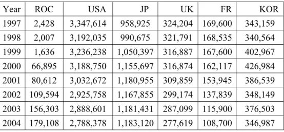
Table 1-4: Case number of traffic accidents over the world from 1997 to 2008

Year ROC USA JP UK FR KOR

1997 2,428 3,347,614 958,925 324,204 169,600 343,159 1998 2,007 3,192,035 990,675 321,791 168,535 340,564 1999 1,636 3,236,238 1,050,397 316,887 167,600 402,967 2000 66,895 3,188,750 1,155,697 316,874 162,117 426,984 2001 80,612 3,032,672 1,180,955 309,859 153,945 386,539 2002 109,594 2,925,758 1,167,855 299,174 137,839 348,149 2003 156,303 2,888,601 1,181,431 287,099 115,900 376,503 2004 179,108 2,788,378 1,183,120 277,619 108,700 346,987

5 2005 203,087 2,699,000 1,156,633 267,816 108,000 342,233 2006 211,176 2,575,000 1,098,199 255,232 102,100 340,229 2007 216,927 2,491,000 1,034,445 244,834 103,200 335,906 2008 227,423 - 945,504 228,367 - -

1.3 Objective

The collision accidents between vehicle and other generalized obstacles occur frequently during backing up period. Therefore, developing obstacle detection technique to prevent the crash accident is our main purpose. In our research, the obstacle which we want to detect is any object that can obstruct the vehicle’s driving path or anything raising out significantly from the road surface. Therefore, the objective of our research is to develop a monocular vision-based obstacle detection algorithm on rear-view for improving backing-up maneuver safety. Adopting the advantages of vision-based obstacle detector, which have longer and wider detection range relative to radar, and that visual display can help driver to know position of obstacle and to indicate the distance away from ego-vehicle further more. Besides, we expect to utilize single camera to achieve obstacle detection not to adopt stereo vision, because low cost relative to stereo vision is considered. Then we intend to detect obstacle effectively for general environment and estimate the distance between target position and ego-vehicle accurately to alarm the driver. By proposing the obstacle detection for backing up, we want to prevent some backing-up crashes and to improve the safety.

1.4 Thesis Organization

6

works about IPM and obstacle detection. Chapter 3 introduces system overview and some fundamental techniques such as IPM and optical flow. Chapter 4 shows obstacle detection algorithm including feature point extraction, ground movement estimation, obstacle localization, obstacle verification and distance measurement. Chapter 5 shows experimental results and evaluations. Finally, the conclusions of this system and future work will be presented in chapter 6.

7

Chapter 2.

Related Works

2.1 Related Works of Inverse Perspective Mapping

(IPM)

The objective of inverse perspective mapping method is to remove the perspective effect caused by camera. This effect will cause the far scene to be condensed and always make following processing to be confused.

The main team who researched about the application of inverse perspective mapping topic are Alberto Broggi’s team at the University of Parma in Italy. First, they proposed an inverse perspective mapping theory and establish the formulas [5]. Then they use these theories combine with some image processing algorithm, stereo camera vision system, and parallel processor for image checking and analysis (PA-PRICA) system which works in single Instruction multiple data (SIMD) computer architecture to form a complete general obstacle and lane detection system called GOLD system [6]. The GOLD system which was installed on the ARGO experimental vehicle is in order to achieve the goal of automatic driving.

There are other researchers using the inverse perspective mapping method [5] or similar mapping method combining with other image processing algorithm to detect lane or obstacles. For example, W. L. Ji [7] utilized inverse perspective mapping to get the 3D information such as the front vehicle height, distance, and lane curvature. Cerri et al. [8] utilized stabilized sub-pixel precision IPM image and time correlation to estimate the free driving space on highways. Muad et al. [9] used inverse perspective mapping method to implement lane tracking and discussed the factors which influent IPM. Tan et al. [10] combined the inverse perspective mapping and

8

optic flow to detect the vehicle on the lateral blind spot. Jiang et al. [11] proposed the fast inverse perspective mapping algorithm and used it to detect lanes and obstacles. Nieto et al. [12] proposed the method that stabilized inverse perspective mapping image by using vanish point estimation. Yang [13] adjusted the characteristic of inverse perspective mapping proposed by Broggi [5], which is the property a horizontal straight line in the image will be projected to an arc on the world surface. However, a horizontal straight line in the image will be projected to a straight line on the world surface, and a vertical straight line in the image will also be projected to a straight line and the prolongation will pass the camera vertical projection point on the world surface.

2.2 Related Works of Obstacle Detection

The obstacle detection is the primary task for intelligent vehicle on the road, since the obstacle on the road can be approximately discriminated from pedestrian, vehicle, and other general obstacles such as trees, street lights and so on. The general obstacle could be defined as objects that obstruct the path or anything located on the road surface with significant height.

Depending on the number of sensors being used, there are two common approaches to obstacle detection by means of image processing: those that use a single camera for detection (monocular vision-based detection) and those that use two (or more) cameras for detection (stereo vision-based detection).

The stereo vision-based approach utilizes well known techniques for directly obtaining 3D depth information for objects seen by two or more video cameras from different viewpoints. Koller et al. [14] utilized disparities in correspondence to the

9

obstacles to detect obstacle and used Kalman filter to track obstacles. A method for pedestrian(obstacle) detection is presented in [15] whereby a system containing two stationary cameras. Obstacles are detected by eliminating the ground surface by transformation and matching the ground pixels in the images obtained from both cameras. The stereo vision-based approaches have the advantage of directly estimating the 3D coordinates of an image feature, this feature being anything from a point to a complex structure. The difference in viewpoint position causes a relative displacement, called disparity, of the corresponding features in the stereo images. The search for correspondences is a difficult, time-consuming task that is not free from the possibility of errors. Therefore, the performance of stereo methods depends on the accuracy of identification of correspondences in the two images. In other words, searching the homogeneous points pair in some area is the prime task of stereo methods.

The monocular vision-based approaches utilize techniques such as optical flow. For optical flow based methods which indirectly compute the velocity field and detect obstacle by analyzing the difference between the expected and real velocity fields, Kruger et al. [16] combined optical flow with odometry data to detect obstacles. However, optical flow based methods have drawback of high computational complexity and fail when the relative velocity between obstacles and detector are too small. Inverse perspective mapping (IPM), which is based on the assumption of moving on a flat road, has also been applied to obstacle detection in many literatures. Ma et al. [17][18][19] present an automatic pedestrian detection algorithm based on IPM for self-guided vehicles. To remove the perspective effect by applying the acquisition parameters (camera position, orientation, focal length) on the assumption of a flat road geometry, and predicts new frames assuming that all image points lie on the road and that the distorted zones of the image correspond to obstacles. Bertozzi et

10

al. [20] develop a temporal IPM approach, by means of inertial sensors to know the speed and yaw of the vision system and the assumption of flat road. A temporal stereo match technique has been developed to detect obstacles in moving situation. Although these methods could utilize the property of IPM to obtain effective results, but all of these should rely on external sensors such as odometer or inertial sensor to acquire ego-vehicle’s displacement on the ground that enables them to compensate movement over time for the ground plane. Yang et al. [21] proposed a monocular vision-based approach by compensating for the ground movement between consecutive top-view images using the estimated ground-movement information and computes the difference image between the previous compensated top-view image and the current top-view image to find the obstacle regions. Therefore, we want to propose a pure vision-based algorithm only use a single camera and does not need additional sensor that could detect the target object for general environment.

11

Chapter 3

System Overview and Fundamental

Techniques

3.1 System Overview

The overall system flowchart is shown in Fig. 3-1 and Fig. 3-2. At the beginning, we will utilize the road detection technique to support the feature point extraction. Due to the characteristic of color space, we first transform the RGB images to Lab color space. The road detection algorithm is processed on Lab color space. Then, we analysis the features which are suitable for track in our condition, the road boundary and the features which gradient is satisfied the restriction in the road region is selected, and the detailed contents will be described in Section 4.1.

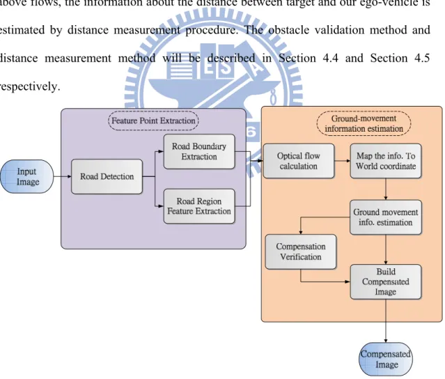
While we are obtaining the feature points, the optical flow will be calculated among all of the feature points. Due to the perspective effect, the direction and length of the optical flows on the road in the original image are not the same. Therefore, we transform the information include the image coordinate and optical flow of feature points from the image coordinate to the world coordinate by inverse perspective mapping(IPM) [13] and build the bird’s view image. When we obtain the information of feature points in world coordinate, the principal distribution of optical flow and the temporal coherence is used to estimate and verify the ground movement respectively. By transforming coordinate between image coordinate and world coordinate and compensating the ground movement, we can build a compensated image which is shifted by ground movement. The ground movement compensation procedure will be shown in Section 4.2 in detail.

12

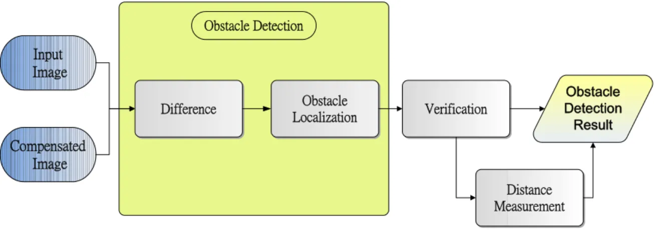
As depicted in Fig. 3-2, the obstacle localization procedure is done by image difference. By thresholding the image, we can obtain the obstacle candidate image which the planar object in the image will be eliminated and the non-planar object which is the obstacle regions will be marked. For each obstacle region the closest position to our ego-vehicle is the interesting. The objective of obstacle localization is to look for the closest position and we can warn the driver by showing the target position. The detail of the obstacle localization will be described in Section 4.3. To ensure the detection results whether the objects are obstacles or not, we utilize the road detection result to validate the initial results. When the objects are detected by above flows, the information about the distance between target and our ego-vehicle is estimated by distance measurement procedure. The obstacle validation method and distance measurement method will be described in Section 4.4 and Section 4.5 respectively.

13 Input Image Compensated Image Difference Obstacle Localization Verification Obstacle Detection Result Obstacle Detection Distance Measurement

Fig. 3-2 System Flowchart

As mentioned above, ground movement information is estimated from optical flow in the world coordinate system and used to compensation for the difference between consecutive frame images in the world coordinate. Therefore, the inverse perspective mapping (IPM) and optical flow techniques adopted in our system will be introduced in the next section 3.2 and 3.3 respectively.

3.2 Inverse Perspective Mapping (IPM)

The perspective effect associates different meanings to different image pixels, depending on their position in the image. Conversely, after the removal of the perspective effect, each pixel represents the same portion of the information content, allowing a homogeneous distribution of the information among all image pixels. In other words, a pixel in the lower part of the image represents less information, while a pixel in the middle of the same image involves more information.

To cope with the effect that non-homogenous information content distribution among all pixels, an inverse perspective mapping transformation method will be introduced to remove perspective effect. To remove the perspective effect, it is

14

necessary to know the specific acquisition conditions (camera position, orientation, optics, etc.) and the scene represented in the image (the road, which is now assumed to be flat). This constitutes the a priori knowledge. The procedure aimed to remove the perspective effect by resample the incoming image, remapping each pixel on the original camera’s image toward a different position and producing a new two-dimensional (2-D) array of pixels. The resulting image represents a top view of the scene, as it was observed from a significant height. Hence we will obtain a new image whose pixels indicate homogeneous information content.

In our research, the inverse perspective mapping [13], which will be able to remove the perspective effect by transforming the image coordinate to world coordinate and then process upon the world coordinate to estimate ground movement.

With some prior knowledge such as the flat road assumption and intrinsic and extrinsic parameters, we will be able to reconstruct a two-dimension image without perspective effect. The expectative results of diagrams are shown in Fig. 3-3. The transformation equation pair [13] with two expectative results: (1) a vertical straight line in the image will still be projected to a straight line whose prolongation will pass the camera vertical projection point on the world surface, (2) a horizontal straight line in the image will be projected to a straight line instead of an arc on the world surface. This result can be verified by similar triangle theorem.

15 (a)

(b) (c)

Fig. 3-3: The expectative results of diagrams (a) perspective effect removing (b) the property of a vertical straight line (c) the property of a horizontal straight line

The spatial relationship between the world coordinate and image coordinate system is shown in Fig. 3-4, and the illustrations of deriving process shown in Fig. 3-5

16 x η y η x

η

(a) (b)

Fig. 3-4: (a) Bird’s view and (b) side view of the geometric relation between world coordinate and image coordinate system.

From Fig. 3-5, the following equations will be derived β β θ -1 -m 2 u 1 = → α α θ -1 -n 2 v 2 = → (3-1) x

η

Fig. 3-5: Geometric relation of image coordinate system and world coordinate system The forward transformation equations will be derived, and the backward transformation equations are easily obtained by some mathematical computation. The

17

forward transformation and backward transformation equations are shown below:

Forward transformation equations:

1 1 2

X H*cot(

θ θ

)*cos( ) H*csc(

γ

θ θ

)*tan( )*sin( )

θ

γ

⇒ =

+

+

+

1 1 2

Y -H*cot(

θ θ

)*sin( ) H*csc(

γ

θ θ

)*tan( )*cos( )

θ

γ

⇒ =

+

+

+

(3-2) Backward transformation equations:

) -) H ) sin( * Y -) cos( * X ( (cot * 2 1 -m u -1 γ γ _{θ β} β + = ⇒ ) ) ) csc( * H ) cos( * Y ) sin( * X ( (tan * 2 1 -n v 1 1 - _α θ θ γ γ α + + + = ⇒ (3-3) The notations in the above equations and figures are introduced as follows:

(u,v) : The image coordinate system.

(X,Y,Z) : The world coordinate system where (X,Y,0) represent the road surface. (L,D,H) : The coordinate of camera in the world coordinate system.

θ: The camera’s tilt angle. γ: The camera’s pan angle.

β

α

, : The horizontal and vertical aperture angle. m,n : The dimension of image (m by n image). O: The optic axis vector.

y x,η

η : The vector which represents the optic axis vector O projected on the road

surface and its perpendicular vector.

To implement the inverse perspective mapping, we use the equations (3-3) instead of equations (3-2) and scan row by row on the remapped image to compute

18

the mapping points on the original image while we do not want an image full of hollows. However, the objective of inverse perspective mapping in our research is not to build the bird’s view image, but aiming to use the transformation to remove the perspective effect and to transform coordinate between the original image coordinate and the world coordinate system. By utilizing inverse perspective mapping, the ground movement estimation procedure will process in the world coordinate system.

3.3 Optical Flow

When we are dealing with a video source, as opposed to individual still images, we may often want to assess motion between two frames (or a sequence of frames) without any other prior knowledge about the content of those frames. The optical flow itself is some displacement that represents the distance a pixel has moved between the previous frame and the current frame. Such a construction is usually referred to as a dense optical flow, which associates a velocity with every pixel in an image. The Horn-Schunck method [22] attempts to compute just such a velocity field. One seemingly straightforward method simply attempting to match windows around each pixel from one frame to the next; this is known as block matching. Both of these methods are often used in the dense tracking techniques.

In practice, calculating dense optical flow is not easy. Consider the motion of a white sheet of paper. Many of the white pixels in the previous frame will simply remain white in the next. Only the edges may change, and even then only those perpendicular to the direction of motion. The result is that dense methods must have some method of interpolating between points that are more easily tracked so as to solve for those points that are more ambiguous. These difficulties manifest themselves

19

most clearly in the high computational costs of dense optical flow.

This leads us to the alternative option, sparse optical flow. Algorithms of this nature rely on some means of specifying beforehand the subset of points that are to be tracked. If these points have certain desirable properties, such as the “corners”, then the tracking will be relatively robust and reliable. The computational cost of sparse tracking is so much less than dense tracking that many practical applications are often adopting. Therefore, we consider the most popular sparse optical flow technique, Lucas-Kanade (LK) optical flow [23][24], this method also has an implementation that works with image pyramids, allowing us to track faster motions.

The Lucas-Kanade (LK) algorithm, was applied to a subset of the points in the input image, it has become an important sparse technique. The LK algorithm can be applied in a sparse context because it relies only on local information that is derived from some small window surrounding each of the points of interest. The disadvantage of using small local windows in Lucas-Kanade is that large motions can move points outside of the local window and thus become impossible for the algorithm to find. This problem led to development of the “pyramidal” LK algorithm, which tracks starting from highest level of an image pyramid (lowest detail) and working down to lower levels (finer detail). Tracking over image pyramids allows large motions to be caught by local windows.

The basic idea of the LK algorithm rests on three assumptions:

1. Brightness constancy. A pixel from the image of an object in the scene does not change in appearance as it (possibly) moves from frame to frame. For grayscale images, this means we assume that the brightness of a pixel does not change as it is tracked from frame to frame.

2. Temporal persistence. The image motion of a surface patch changes slowly in time. In practice, this means the temporal increments are fast enough relative to the scale

20

of motion in the image that the object does not move much from frame to frame. 3. Spatial coherence. Neighboring points in a scene belong to the same surface, have

similar motion, and project to nearby points on the image plane.

By using these assumptions, the following equation can be yielded, where y component of velocity is v and the x component of velocity is u:

0

x y t

I u+I v+ =I (3-4)

For this single equation there are two unknowns for any given pixel. This means that measurements at the single-pixel level cannot be used to obtain a unique solution for the two-dimensional motion at that point. Instead, we can only solve for the motion component that is perpendicular to the line described by the flow equation. Fig. 3-6 presents the mathematical and geometric details.

0

T x y t t

I u

+

I v

+ =

I

⇒ ∇

I u

= −

I

x y I u u I I v ⎡ ⎤ ⎡ ⎤ =_{⎢ ⎥ ∇ = ⎢ ⎥} ⎣ ⎦ ⎣ ⎦ (3-5) t I I − ∇

Fig. 3-6: Two-dimensional optical flow at a single pixel:optical flow at one pixel is underdetermined and so can yield at most motion, which is perpendicular to the line

described by the flow equation

21

have a small aperture or window in which to measure motion. When motion is detected with a small aperture, you often see only an edge, not a corner. But an edge alone is insufficient to determine exactly how (i.e., in what direction) the entire object is moving. To resolve the aperture problem, we turn to the last optical flow assumption for help. If a local patch of pixels moves coherently, then we can easily solve for the motion of the central pixel by using the surrounding pixels to set up a system of equations. For example, if we use a 5-by-5 window of brightness values, round the current pixel to compute its motion, we can then set up 25 equation as follows: { 1 1 1 2 2 2 25 25 25 ( ) ( ) ( ) ( ) ( ) ( ) ( ) ( ) ( ) x y t x y t x y t I p I p I p I p I p u I p v I p I p d I p b A ⎡ ⎤ ⎡ ⎤ ⎢ ⎥_{⎡ ⎤} ⎢ ⎥ ⎢ ⎥_{⎢ ⎥=}⎢ ⎥ ⎢ ⎥_{⎣ ⎦} ⎢ ⎥ ⎢ ⎥ ⎢ ⎥ ⎢ ⎥ ⎣ ⎦ ⎣ ⎦ M M M 14243 144424443 (3-6) To solve for this system, we set up a least-squares minimization of the equation, wherebymin Ad−b 2 is solved in standard form as: ( T ) T

A A d =A b. From this relation we obtain our u and v motion components. Writing this out in more detail and the solution to this equation is yielded:

1 ( ) T _T t x x x x y T T x y y y _y t A A _{A b} I I I I I I u u A A A b I I I I v I I v − ⎡ ⎤ ⎡ ⎤ ⎡ ⎤ ⎡ ⎤ = −⎢ ⎥ ⇒ = ⎢ ⎥ ⎢ ⎥ ⎢ ⎥ ⎢ ⎥ ⎣ ⎦ ⎣ ⎦ ⎣ ⎦ _{⎣ ⎦}

∑

∑

∑

∑

∑

∑

144424443 ₁₄₂₄₃ (3-7)

22

Chapter 4

Obstacle Detection Algorithm

4.1 Feature Point Extraction

4.1.1 Feature Analysis

There are many kinds of local features that one can track. Features which are used to estimate ground movement based on its motion, that is to find these features from one frame in a subsequent frame of the video stream. Obviously, if we pick a point on a large blank wall then it won’t be easy to find that same point in the next frame of a video. If all points on the wall are identical or even very similar, then we won’t have much luck tracking that point in subsequent frames. On the other hand, if we choose a point that is unique then we have a pretty good chance of finding that point again. In practice, the point or feature we select should be unique, or nearly unique, and should be parameterizable in such a way that it can be compared to other points in another image. Therefore, we might be tempted to look for points that have some significant change within neighboring local area that is the good features which have a strong derivative in spatial domain. Another characteristic of features is about the position of the image. Due to the objective of the following procedure is to estimate the ground movement information, features lie on the ground region is useful for the following ground movement estimation algorithm. According to above analysis, a good feature to track should have two characteristics. First, a feature should have strong derivative which could assist us to track them and obtain a precise motion. Then, the position of feature should be restricted on the road region (non-obstacle region). The features which we will use them to estimate the ground

23

movement information should conform the above two characteristic, these features will be suitable for estimating ground movement information.

To consider the first characteristic – strong derivative, a point to which a strong derivative is associated may be on an edge of some kind. Then considering this property of edge we employ the Sobel operator to find out the edge of image. The points which be extracted by edge detection are used to be feature points, which then calculate optical flow for all of these feature points. These edge points and its optical flow of image is shown in Fig. 4-1. But a problem is arising as depicted in Fig 4-1(b), it could look like all of the other points along the same edge. An ambiguous optical flow will happen when the edge points parallel to the direction of motion. It turns out that strong derivative of a single direction is not enough. However, if strong derivatives are observed in two orthogonal directions then we can hope that this point is more likely to be unique. For this reason, many trackable features in the image that are corners. Intuitively, corners are the points that contain enough information to be picked out from one frame to the next. We examined by the most commonly used definition of a corner was provided by Harris[25]. This definition relies on the matrix of the second-order derivatives (∂2x, ∂2 y, ∂x∂y) of the image intensities. We can think

of the second-order derivatives of images, taken at all points in the image, as forming new second-derivative images or, when combined together, a new Hessian image. This terminology comes from the Hessian matrix around a point, which is defined in

two dimensions by:

2 2 2 2 2 2 I ( ) I x x y H p I I y x y ⎡ ∂ ∂ ⎤ ⎢ _{∂ ∂ ∂} ⎥ ⎢ ⎥ = ⎢ _{∂ ∂} ⎥ ⎢_{∂ ∂ ∂} ⎥ ⎣ ⎦ (4-1)

By using Harris corner definition, the result of corner detection and its corresponding optical flow is shown Fig. 4-2. It is obvious to observe that motion of corner is

24

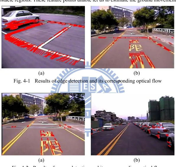
relative accurate than edge point. Although corner have more precise optical flow, another problem is arising that is position of corner almost lie on obstacle region such as vehicle component. The Fig. 4-2(b) is shown the result of corner detection in a common driving condition, we can see that the feature points are nearly located on obstacle regions. These feature points unable let us to estimate the ground movement.

(a) (b)

Fig. 4-1 Results of edge detection and its corresponding optical flow

(a) (b)

Fig. 4-2 Results of corner detection and its corresponding optical flow

By considering above analysis of features, we proposed a feature point extraction method employ road detection procedure to assist in getting ground features. The flowchart of proposed feature point extraction is shown in Fig. 4-3. The objective is to distinguish the major road region and non-road region, and utilize the result of the road detection, that is to extract the boundary of major road and some good features within road region. By integrating road detection, the more useful ground features

25

could be extracted and could improve results of ground movement effectively. The next chapter 4.1.2 will introduce the detail of road detection and describe what feature point will be selected.

Previous

frame Road Detection

Road Boundary Extraction

Road Region Feature Extraction Feature Point Extraction

Feature point info. Major Road

Component Extraction

Fig. 4-3 Flowchart of feature point extraction

4.1.2 Road Detection

The proposed feature point extraction technique is integrating a road detection procedure [26] which is used an on-line color model that we can train an adaptive color model to fit road color. The main objective of road detection is to discriminate the road and non-road region roughly, because the result is used to support feature extraction not used to extract obstacle regions. However, we adopt an on-line learning model that allows continuously update during driving, through the training method that can enhance plasticity and ensure the feature is on the road region.

Due to the color appearance in the driving environment, we have to select the color features and using these color features to build a color model of the road. Therefore, we have to choose a color space which has uniform, little correlation, concentrated properties in order to increase the accuracy of the model. In computer color vision, all visible colors are represented by vectors in a three-dimensional color

26

space. Among all the common color spaces, RGB color space is the most common color feature selected because it is the initial format of the captured image without any distortion. However, the RGB color feature is high correlative, and the similar colors spread extensively in the color space. As a result, it is difficult to evaluate the similarity of two color from their 1-norm or Euclidean distance in the color space.

The other standard color space HSV is supposed to be closer to the way of human color perception. Both HSV and L*a*b* resist to the interference of illumination variation such as the shadow when modeling the road area. However, the performance of HSV model is not as good as L*a*b* model because the road color cause the HSV model not uniform that lead to the HSV color model not as uniform as the L*a*b* color model. There are many reasons attribute this result. Firstly, HSV is very sensitive and unstable when lightness is low. Furthermore, the Hue is computed by dividing (Imax - Imin) in which Imax = max(R,G,B), Imin = min(R,G,B), therefore

when a pixel has a similar value of Red, Green and Blue components, the Hue of the pixel may be undetermined. Unfortunately, most of the road surface is in similar gray colors with very close R, G, and B values. If using HSV color space to build road color model, the sensitive variation and fluctuation of Hue will generate inconsistent road colors and decrease the accuracy and effectiveness. L*a*b* color space is based on data-driven human perception research that assumes the human visual system owing to its uniform, little correlation, concentrate characteristics are ideally developed for processing natural scenes and is popular for color-processed rendering. L*a*b* color space also possesses these characteristics to satisfy our requirement. It maps similar colors to the reference color with about the same differences by Euclidean distances measure and demonstrates more concentrated color distribution than others. Then considering the advantaged properties of L*a*b* for general road environment, the L*a*b* color space for road detection is adopted.

27

The RGB-L*a*b* conversion is described as follow equations: 1. RGB-XYZ conversion: 0.431 0.342 0.178 X = ⋅ +R ⋅ +G ⋅B 0.222 R+0.707 G+0.071 B Y = ⋅ ⋅ ⋅ 0.020 0.130 0.939 Z = ⋅ +R ⋅ +G ⋅ B 2. Cube-root transformation: 1 3 1 3 * 166 16 >0.008856 * 903.3 0.008856 * 500 [ ( ) ( )] * 200 [ ( ) ( )] X , , , XYZ n n n n n n n n n n n Y Y L if Y Y Y Y L if Y Y X Y a f f X Y Y Z b f f Y Z

where Y Z are tristimulus values of reference white poi

⎧ _{⎛ ⎞} ⎪ _{= ⋅⎜ ⎟ −} ⎪⎪ ⎝ ⎠ ⎨ ⎪ _{⎛ ⎞} ⎪ = ⋅_{⎜ ⎟} ≤ ⎪ _{⎝ ⎠} ⎩ = ⋅ − = ⋅ − 1 3 _>0.008856 ( ) 7.787 16 /116 0.008856 n n n n n nt X = 95.05,Y = 100,Z = 108.88 Y t Y f x Y t Y ⎧ ⎪ ⎪ = ⎨ ⎪ _{+ ≤} ⎪⎩

By modeling and updating of the L*a*b* color model, the built road color model can be used to extract the road region. The L*a*b* model is constituted of K color balls, and each color ball mi is formed by a center on ( ,* ,* )

i i i

m m m

L a b and a fixed

radiusλ_max =5 as seen in Fig. 4-4. In order to train a color model, we set a fixed area of the lower part of the image and assume pixels in the area are the road samples. For each of these pixels in the beginning 30 frames are used to initialize the color model, and updating the model every ten frames to increase processing speed but still maintain high accurate performance.

28

Fig. 4-4 A color ball i in the L*a*b* color model whose center is at (Lm, *am, *bm)

and with radius λ _max

The sampling area is used to be modeled by a group of K weighted color balls. We denote the weight and the counter of the mi th color ball at a time instant t by Wm ti,

and _,

i

m t

Counter , and the weight of each color ball represents the stability of the color.

The color ball which more on-line samples belonged to over time accumulated a bigger weight value shown in Fig. 4-5. Adopting the weight module increases robustness of the model.

Fig. 4-5 Sampling area and color ball with a weight which represents the similarity to current road color.

29

The weight of each color ball is updated by its counter when the new sample is coming which is called one iteration. Therefore the counter would be initialized to zero at the beginning of iteration. The counter of each color ball records the number of pixels added from the on-line samples in the iteration. The first thing to do is that which color ball is chosen to be added. We measure the similarity between new pixel xt and the existing K color balls using a Euclidean distance measure (4-1). The

maximum value of K is 50 which represents each on-lined model contains 50 color balls at most. 2 2 2 max ( , ) ( ) ( ) ( ) i i i i m x m x m x Similarity x m =sqrt_⎣⎡ L −L + a −a + b −b ⎤_⎦<=λ (4-1)

If a new pixel xt was covered by any of the color ball in the model, one will be

added to the counter of best matching color at this iteration as the equation (4-2). After entire new sample pixels at this iteration undertake the matching procedures mentioned above, the weights of every color ball are updated according to their current counter and their weight at last iteration. The updating method is as follows:

i i m i i max m(x )= arg min(Similarity(x ,m ) <=λ ) (4-2) , 1 (1 ) / [0,1], i i m t w t w m sample w sample W W counter N N α α α + = ⋅ + − ⋅ ∈

, where α is user-defined learning rate, N_w sample is the sampling area

Then using the weight to decide which color ball of the model most adapt and resemble current road. The color balls are sorted in a decreasing order according to their weights. As a result, the most probable road color features are at the top of the list. The first B color balls are selected to be enabled as standard color for road detection, and these color balls with a higher weight has more importance in detection

step B st mat dete dete road the whi posi so o p. Road dete tandard colo tch is found ected as roa Fig. 4 Fig. 4-7 sh ermined as d detection world coor ich is cause ition in the on). ection is ac or balls sele d, the pixel x ad. 4-6 Pixel ma hows some road else a to all of th rdinate, that ed by the ge image due hieved via ected at the xt is consid atched with represe results of o are the non e image bec t is the ran eometrical c to camera s 30 comparison previous in dered as non first B weig ent standard on-line L*a* n-road regio cause of the nge of road characterist set up envir n of the new nstant of tim n-road. On t ght color ba d color. *b* road de ons. Howev e following detection i tic of IPM, ronment (ca w pixel xt w me shown in the contrary alls which a etection, the ver, we will g procedure is restricted and could b amera heigh

with the exis n Fig. 4-6. I y, the pixel

are the most

green areas l not under is processe d to the hor be the diffe ht, tilt angle sting If no xt is t s are rtake ed in rizon erent e and

4.1

regi con bou regi is u conn Afte that to b feat maj poin coll is s supp

1.3 Featu

The objec ion, and the sider the tw undary and s Therefore ion. When r used to mer nected com er that we w t to be the m be feature p ture and ha or road are nts because lected comp hown some port feature

ure Point

ctive of roa e result will wo character strong gradi , the first s result of roa rge the neig mponent is e

will find ou major road r points, beca

ve strong d ea, and the e of their st pletely by th e results of e point extra Fig. 4-7

t Extrac

ad detection l be used to ristics that a ient points a step of featu ad detection ghboring re executed to ut the maxim region. The ause the bo derivative. B more stron trong deriv hese road b f feature po action, the m 31 Results of r

ction

n is to disti o extract fe are strong d are selected ure point ex n is obtaine egion and t separate the mum compo en the bound order of ro Besides, we g gradient p vative and p oundary an oint extracti more useful road detecti inguish the eature point derivative an d to be featu xtraction is ed, the dilat to reduce th e road regio onent of all dary of maj ad and non e analyze th points will position. Th nd high grad ion. By em ground fea ion major road . As above nd ground f re points. s to extract

tion and ero he fragmen ons to sever l componen jor road reg n-road shou he gradient

be extracte hen the fea dient feature mploying ro tures can be d and non-mentioned feature, the the major osion proce ntation then ral compone nts and assu gion is extra uld be the t distributio ed to be fea ature points es. The Fig. oad detectio e extracted. road d, we road road dure n the ents. umed acted road on of ature s are . 4-8 on to

32

Fig. 4-8 Results of feature point extraction. The upper image is result of road detection, and lower image is position of feature points.

 

4.2 Ground Movement Estimation

In this section we will introduce the proposed ground movement estimation procedure. Ground movement information is estimated from optical flow in the world coordinate system. By analyzing the principal distribution of optical flow can let us get the most representative ground movement, which will be used to compensate for the previous frame and difference with current frame. In addition, ground movement will be verified via temporal coherence. The flow of ground movement estimation is illustrated in Fig. 4-9.

33

Map the info. To World coordinate Ground movement info. estimation Build Compensated Image Compensation Verification Compensated Image Feature

point info. Optical flowcalculation

Fig. 4-9 flow of ground movement estimation

4.2.1 Ground Motion Estimation

By feature point extraction procedure as described in section 4.1, the useful features for ground movement estimation is obtained. Then these feature points will be used to estimate ground motion. Therefore, when the feature points are acquired the main tasks of ground movement estimation procedure are high accuracy optical computation and ground movement information estimation. The first step is to calculate the optical flow for all of these feature points. The pyramidal Lucas and Kanade algorithm introduced in section 3.3, which copes efficiently with large movements, is used to calculate the optical flow for these feature points in the original image. As a result, Fig. 4-10(a) and Fig. 4-11(a) shows the feature points and its corresponding optical flow in the original image. Due to the perspective effect, the directions and lengths of the optical flows on the road in the original image are not the same when vehicle is moving straight shown in Fig. 4-10(a). The case in which the

34

vehicle is turning is shown in Fig. 4-11. In this case the complicated optical flow distribution appeared in the original image. However, the inconsistent optical flow of road in the original image let us encounter a difficulty to estimate the ground movement. Therefore, we will take advantage of the IPM to remove the perspective effect. The optical flow information of an original image is mapped into world coordinate. The objective of inverse perspective mapping (IPM) is to remove the perspective effect by transforming the image coordinate to world coordinate, and scale the world coordinate that can obtain a bird’s view image. Therefore, the world coordinate information is same as bird’s view image that both of them are perspective removal. In our research, the IPM is used to remove the perspective effect and transform the image coordinate information to world coordinate and the ground movement procedure is processed in the world coordinate the bird’s view image is used to display and examine some results, which we will not process on it.

The difference between the optical flow of the original image and that of the bird’s view image is shown in Fig. 4-10 and Fig. 4-11. When a vehicle is moving straight, the optical flows in the bird’s view image have the same direction and length independent of the locations of the optical flows. Similarly when vehicle is turning, the optical flow distribution in the bird’s view image draws concentric circle following the movement of the ground but roughly have a similar magnitude.

(a) optical flows of original image (b) optical flows of bird’s view image Fig. 4-10 Difference between optical flow of original image and those of bird’s view

35

image when vehicle is moving straight.

(a) optical flows of original image (b) optical flows of bird’s view image Fig. 4-11 Difference between optical flow of original image and those of bird’s view

image when vehicle is turning.

The kernel concept of ground compensation based detection algorithm is adopting the following characteristics. The optical flow distribution of ground region is approximately consistent in the bird’s view image. On the contrary, a vertical straight line in the image which represented the vertical edge of obstacle in the world coordinate system is projected to a straight line whose prolongation will pass the camera vertical projection point on the world surface. Therefore, the optical flow distribution of obstacle regions are different drastic to the ground region. Then we can estimate the ground movement and used build a compensated image which assume the image is all planar object (ground). Therefore, the planar region will be eliminated but the obstacle regions will not. Fig. 4-12 shows the difference between optical flow of obstacle and those of planar object.

36

Fig. 4-12 Differences between optical flows of obstacle and those of planar object. Thanks to the mapping between original image and world coordinate system, ground movement information can be estimated based on the optical flow of feature points in the world coordinate system. The feature points which we obtained via integrating road detection are with a characteristic that most of these features will lie on ground region. Besides, the specific optical flow distribution of ground region in the world coordinate system, that is optical flow of them will approximately consistent. Due to the above characteristics, we would like to find out the principal distribution of optical flow that can let us get the most representative ground motion. We analyzing the principal distribution of optical flow by calculating the histogram of optical flow according to its direction and magnitude, and the peak of the histogram is considered to be ground motion. As shown in Fig. 4-13, that is the histogram distribution of corresponding optical flow. By utilizing the principal motion, that can let us avoid some errors such as ambiguous optical flow or the non-peak value of optical flow is possibly causing by obstacle feature point.

37

4.2.2 Compensated Image Building

The specific optical flow distribution in the world coordinate system shows that the movement of ground in the world coordinate system can be described as a translation or rotation of a two-dimensional coordinate plane. The ground movement information is estimated by using optical flow in world coordinate system, and the optical flow is ground motion which is estimated by analyzing the principal distribution of optical flow of feature points, that is utilized the procedure as described in last section 4.2.1. Then we can acquire ground motion in the world coordinate system which is used to estimate ground movement information.

In the world coordinate system converted from consecutive images captured at difference location O1 and O2 as depicted in Fig. 4-14, if we represent the world coordinates of a ground feature point P as (x1, y1)T and (x2, y2)T before and after

vehicle movement respectively, the optical flow of the feature point P can be written as Eq. (4-3). 2 1 2 1 x y f x x f y y ⎛ ⎞ ⎛ ⎞ ⎛ ⎞ = − ⎜ ⎟ ⎜ ⎟ ⎜ ⎟ ⎝ ⎠ ⎝ ⎠ ⎝ ⎠ (4-3)

Fig. 4-14 Two-dimensional coordinate plane

38

coordinate system by a two-dimensional coordinate plane as shown in Fig. 4-14, the relationship of corresponding points between consecutive world coordinate system can be described with the Eq. (4-4), where Θ is the rotation component of vehicle movement, and (Tx, Ty)T are the translation components of ground movement. Then

ground movement information including rotation and translation component. That is we can utilize Eq. (4-4) to find out the compensated coordinate of point (x1,y1)T but Θ

and (Tx, Ty)T should be calculated in advance. By substituting Eq. (4-3) into Eq. (4-4),

then the relationship between Θ and (Tx, Ty)T can be derived as Eq. (4-5).

2 1 2 1 cos sin sin cos x y T x x T y y θ θ θ θ − ⎛ ⎞ ⎛ ⎞₌⎛ ⎞⎛ ⎞ + ⎜ ⎟ ⎜ ⎟ ⎜ ⎟⎜ ⎟ ⎝ ⎠ ⎝ ⎠ ⎝ ⎠ ⎝ ⎠ (4-4) 1 1 0 x x y y T f y T f x θ⎛_⎜ ⎞_⎟−⎛ ⎞ ⎛_{⎜ ⎟ ⎜}+ ⎞_⎟= − ⎝ ⎠ ⎝ ⎠ ⎝ ⎠ (4-5)

Where Θ and (Tx, Ty)T are unknown parameters, (fx,fy)T and (y1,-x1)T can be

obtained during the process of optical flow calculation. Therefore, when obtaining the ground motion we can use these ground point information including world coordinate and magnitude of optical flow to calculate the ground movement information, that is unknown parameters Θ and (Tx, Ty)T can be acquired.

By undertaking above procedure, the ground movement information can be obtained and used to interpolate image, then compensated image is generated. Therefore, thanks to the mapping between image coordinate and world coordinate, we will compensate previous frame image to a new image by projecting the image coordinates to the ground plane and compensating the ground movement on the ground plane then back projecting to the image plane again. Fig. 4-15 illustrates the procedure of the compensated image building. For each pixel of the previous frame will be transformed to ground plane which is world coordinate by IPM forward mapping, then for each world coordinate is compensated to new world coordinate by

39

using ground movement information and Eq. (4-4), the coordinates are back transforming to image coordinate by IPM backward mapping, a new image is interpolated in the image plane. Therefore, the new built image is assuming formed by planar object because of compensated using ground movement. Due to these assume the non-planar object (obstacle) can be extracted by comparing current image and compensated image. Image coordinate World coordinate Compensated World coordinate Compensated Image coordinate

Fig. 4-15 procedure of the compensated image building

4.2.3 Compensation Verification

The ground movement information is used to compensate the image and a new image is built. By considering the temporal coherence, that is to consider the condition that the scene will not change a lot during the few frames. For these reason, when the ground movement information is obtained, the compensated image will be built and used to compare with current frame image then we can acquire an obstacle candidate image which indicate the pixel is obstacle or not. The detail of how to generate obstacle candidate image will be introduced in section 4.3. That is number of