同調波轉換於介觀光學與量子力學之研究

國

立

交

通

大

學

電子物理學系

博 士 論 文

同調波轉換於介觀光學與量子力學之研究

Exploring Coherent Wave Transformations in Mesoscopic

Optics and Quantum Mechanics

研 究 生：林毓捷

指導教授：陳永富 教授

Exploring Coherent Wave Transformations in Mesoscopic

Optics and Quantum Mechanics

研 究 生：林毓捷

Student: Yu-Chieh Lin

指導教授：陳永富 教授

Advisor: Prof. Yung-Fu Chen

國立交通大學

電子物理學研究所

博士班論文

A Thesis

Submitted to Institute of Electrophysics

College of Science

National Chiao Tung University

in partial Fulfillment of the Requirements

for the Degree of

PhD

in

Electrophysics

May 2013

Hsinchu, Taiwan, Republic of China

中 華 民 國 一百零二 年 五 月

同調波轉換於介觀光學與量子力學之研究

學生：林毓捷 指導老師：陳永富

國立交通大學電子物理學系博士班

摘要

介觀物理是尺度介於巨觀與微觀的物理科學，使其能涵蓋兩種尺度下的物理特 徵；這一尺度下的物理系統也因此孕育了不少有趣的物理現象為許多不同領域的 科學家們所深深著迷。直至目前為止，相關的議題還是持續地被關注與研究。本 文藉由光在量子(波動光學)與古典(幾何光學)的良好對應性，以光學系統來類比 觀察介於量子力學與古典力學之間的介觀現象。再者，由於描述光學系統的波動 方程式在近軸近似下與研究量子系統的薛丁格波動方程式有相當良好的數學對 應性，在文中我們借助量子力學的理論完備性來探討對應於光波的量子同調態 (quantum coherent states)所具有的物理特性。藉由對量子系統的深入分析，我們 更容易洞悉波動光學與幾何光學之間的奧妙。也藉此更了解量子態在量子系統中 所扮演的重要角色。

文中主要探討同調波在兩種光學系統中的物理面貌，包含光導管(light pipe) 與球型雷射共振腔(spherical laser resonator)。看似完全不同的實驗架構，實際上 卻以相同的理論架構為基礎。由量子同調態疊加的概念配合嚴謹的理論分析，疊 加出來的波函數展現出坐落於古典週期性軌跡(periodic orbit)的物理圖像；透過仔 細的實驗觀察，相同的空間圖像也在光學系統中被驗證。藉由同調態在光學與量 子力學的相互印證之下，更確立了以量子力學為理論基石的進一步相關研究。

converter)，來連結兩群各具特色的光波同調態。而這兩群光波同調態皆具有獨特 的古典週期性粒子軌道形貌，分別是利薩如(Lissajous)曲線和擺線(trochoidal)曲 線。此一研究不僅以視覺化的方式呈現數學研究中拓樸學的內涵，也藉由不同耦 合機制下的二維簡諧系統，具體的展現了粒子軌道的空間對應轉換關係。由於簡 諧系統普遍存在於各個研究領域與問題中，空間轉換同調態的研究與實現想必會 是最直接且容易的途徑來刺激或幫助解答更多不同領域中的相關問題。此外，針 對實驗結果的理論分析更顯示了這些空間模態擁有很大的角動量，這對於未來的 雷射技術提供了一些前瞻性的想法。 而本文另一個探討的議題在介觀物理的研究中一直扮演相當重要的角色，就 是波穿透紊亂介質(disordered medium)所展現出來的局域化(localization)現象。本 文藉由錐形二次諧波產生(conical second harmonic generation)的方式來觀察紊亂 波函數在弱局域化(weak localization)範疇中從遍布態(extended states)到預局域化 態(pre-localized states)的連續性變化；透過理論進一步分析實驗量測到的強度分 布，我們成功地利用縮版的非線性σ模型(reduced version of the nonlinear sigma model)來定量地探討各種形式的強度分布其所對應不同局域化的程度，這是縮版 的非線性σ模型首次在實驗上的一個應用與對照。再者，為人們所熟知的卡方分 布(chi-square distributions)在此一研究中也首次被證實可以有效地使用來定量分 析不同局域化的程度，且與縮版的非線性σ模型有相當良好的對應關係。由於紊 亂系統的實驗並不是很容易觀察，而此一研究提供一個途徑來幫助深入了解紊亂 系統所展現出來的物理圖像；另一方面，實驗結果也意味錐形二次諧波產生的方 式可以協助研究紊亂晶體中複雜的結構特徵。

Exploring Coherent Wave Transformations in

Mesoscopic Optics and Quantum Mechanics

Student: Yu-Chieh Lin Advisor: Prof. Yung-Fu Chen

Institute and Department of Electrophysics

National Chiao-Tung University

Abstract

Mesoscopic physics, which is in between the microscopic and the macroscopic world, contains physical features of both scales. Distinctive phenomena found in the mesosopic systems give insights into the quantum-classical correspondence which has attracted lots of attention from researchers. The related issues in mesoscopic regime have been studying and paying close attention. In the thesis we employed optical systems as analog systems to investigate the connection between quantum and classical mechanics. This statement based on the good correspondence between quantum-classical mechanics and wave-ray optics. Moreover, optical wave equation was theoretically elucidated to be in the same mathematical form as the Schrödinger equation. We provided comprehensive studies for the quantum coherent states corresponding to the optical waves. With sophisticated mathematics in quantum mechanics, we are able to understand the wonderland between wave optics and ray optics and the important roles of quantum coherent states in quantum systems.

Two kinds of optical systems, light pipes and a laser resonator, were discussed in the thesis. Although it seems that the two setups are totally different, they are

governed by the same theoretical foundation. Within rigorous analyses, the coherent states in corresponding quantum systems revealed intriguing patterns localized on the classical periodic orbits. The same spatial patterns could be found in the optical systems. The validation of the connection between quantum and optical coherent waves enables further studies on related research based on quantum mechanics.

Another topic in the thesis is the linkage of two distinctive optical coherent states localized on the periodic orbits of Lissajous and trochoidal curves. The investigation not only visualized the insight of topology in mathematics but exhibited analog transformational relationship of particle trajectories followed by different coupling mechanisms in a two-dimensional harmonic system. Hence, the realization of the converted spatial coherent states might be an accessible method for the study of fundamental science in various branches. With theoretical analyses, the coherent waves were found to carry large orbital angular momentum and might stimulate further applications.

Besides the two topics mentioned on the above, another topic has been played an important role in the mesoscopic physics—the investigation of localization for disordered wave functions in random media. In this work, we obtain the disordered wave functions from the conical second harmonic generation to explore the continuous transformation of weak localization from extended to pre-localized states. We numerically verify that the experimental density distributions with different extents of weak localization can be excellently analyzed with a reduced version of the nonlinear sigma model. This is the first time that the reduced version of the nonlinear sigma model to be applied to describe the experimental results. Moreover, we perform that the chi-square distributions with fractional degrees of freedom are practically equivalent to the density distributions of the reduced version of the nonlinear sigma model. Since the observation of the disordered wave functions is not accessible, this

work might provide an approach to comprehensively study the intriguing physics behind the disordered systems. On the other hand, the present results suggest the possibility of exploiting conical second harmonic generation as a diagnostic method to understand the complex topological structure of the disordered crystals.

誌謝

Acknowledgement

回憶起剛進交大的時候，剛開始接觸大學的普通物理，一直有個刻板印象， “大學物理只是高中物理的英文翻版＂，所以並不會有太大的期待；但上了陳永 富老師的普物課，老師帶給學生的啟發和刺激，讓我又重拾對物理的熱忱。課前 課後，上課的相關內容總要在腦子裡迴盪個 N 遍，即使花了不少時間只能想通 一件事，卻也樂在其中；從大一起就被陳老師的學識與風範所深深吸引，回想之 前為了聽老師課堂以外的分享，不是陳老師導生的我，竟也厚著臉皮去參加老師 的導生聚。除了在大一普物課深受陳老師的啟發外，在之後的日子裡，也追隨了 陳老師，上了老師不少的課程，即使是相同的課程，老師總能傳授給我們新的訊 息與知識；而在大二那年暑假，我就正式加入了陳老師的研究團隊，研究的路上， 充滿驚奇與挑戰，但我很幸運，能一路跟隨陳老師；老師擁有豐富的實作經驗與 深厚的理論功底，總是能適時地引領我、釐清我的盲點；除了研究上的指導，在 待人處事與生活上，老師更是我人生路上的嚮導，面對生活上的挑戰，老師給予 我的關懷與幫助總能讓我放心於研究的路上而不至於蠟燭兩頭燒。再多的文字也 都無法表達我內心對陳老師的感激，但在這裡我還是想要獻上我對陳老師由衷的 感謝。在研究的路上，另一個我想要感謝的老師是黃凱風老師，黃老師在研究上 對我的啟發也扮演相當重要的角色，黃老師擁有深厚的物理背景，因此對於複雜 的物理問題，黃老師總能以清晰簡單的物理圖像，使問題撥雲見日，引領我看到 物理之美；黃老師求知若渴的精神和對研究的熱情更是讓我印象深刻，除了關心 大家的實驗狀況，黃老師不管聚餐還是走在路上，總是論文、學術資料不離手， 隨時跟陳老師熱烈地討論相關的研究議題。兩位老師對研究的熱忱與態度都一點 一滴的烙印在我的內心；當然，要成為一個成熟的研究者，對我來說還有許多要 努力的地方，但我會以兩位老師作為我的標竿榜樣，持續前行。 在研究的路上，除了兩位老師的幫助與教導，還有許多幫助過我的學長姊

們；亭樺學姊，是我的小師父和能一起哭一起笑的好麻吉，不管是研究還是身邊 的五四三總是能話家常，也總是能以大姊大的角度給我適時的提醒與關懷。蘇冠 暐蘇老大，老大總是能用寥寥幾句話就解答我問題的癥結點，不得不佩服他敏銳 的觀察力和精闢的見解與理解力。依萍學姊，細心體貼的她，不管是生活上和研 究上都給予我許多的關心和幫助。興弛學長，在我剛進實驗室時指導我，讓當時 是菜鳥的我在研究上能更快地上手。彥廷學長，在研究上常常提供我相關的意見 和想法，是個很可以分享與討論的對象。還有已經畢業但也給予我相當多協助的 學長姊們，感謝雅婷、家楨、哲彥、仕璋、和漢龍學長。另外也要感謝平時能一 起討論和互相鼓勵的好麻吉小江、威哲、郁仁、舜子和建至，讓我在研究的路上 能擁有一群貼心的夥伴們而並不會感到孤獨；還有實驗室裡的毅帆、易純、段必、 小曄子、咪婷、平平、小佑、奶油、家翰、昱辰、容辰、泰緯、育廷、純甫和文 政，在實驗室裡跟大家一起經歷和分享過的美好時光都將成為我最棒的回憶。 最後我要感謝我最愛也最愛我的家人，感謝我的家人一直以來對我無私地付 出與鼓勵，我期許自己未來能成為他們最強而有力的肩膀與後盾。

Contents

Abstract (Chinese) i

Abstract iii

Acknowledgement vi

Contents viii

List of Figures xi

  Chapter 1Introduction to the Thesis ... 1 

1.1  Classical Mechanics and Ray Optics : Periodic Orbits ... 1 

1.2  Schrödinger Wave Equation and Paraxial Wave Equation ... 2 

1.3  Optical-Mechanical Analogy ... 7 

1.4  Mesoscopic Wave Functions ... 10 

1.4.1 Periodic Orbits in Mesoscopic Systems ... 10 

1.4.2 Disordered Wave Functions in Random Media ... 11 

Reference ... 14 

Chapter 2 Coherent Wave Transformation in Quantum Harmonic Oscillators and Spherical Laser Resonators ... 18 

2.0 Introduction ... 18 

2.1 Coupled Quantum Harmonic Oscillators ... 20 

2.1.1 Eigenstates : SU(2) Transformation ... 21 

2.1.2 Coherent States : Single Periodic Orbits ... 24 

2.1.3 Coherent States : Multiple Periodic Orbits ... 39 

2.2 Analogous Optical Experiments ... 56 

2.2.1 Experimental Setup ... 56 

2.2.2 Eigenmodes : General Huygens’ Integral ... 57 

2.2.3 Coherent Modes: Single Periodic Orbits ... 63 

2.2.4 Coherent Modes : Multiple Periodic Orbits ... 69 

2.3 Extension Topic : Generation of Optical Vortex Array ... 82 

2.3.2 Transformation of Fundamental Laser Modes ... 84 

2.3.3 Formation of Optical Vortex Array ... 86 

2.3.4 Formation of Flower Laguerre-Gaussian Modes ... 91 

2.3.5 Experimental Setup ... 92 

2.3.6 Experimental Results and Discussions ... 94 

2.3.7 Summary ... 96 

Reference ... 102 

Chapter 3 Generation of Resonant Geometric Modes in Quantum Circular Billiards and Light Pipes ... 107 

3.0 Introduction ... 107 

3.1.1 Eigenstates ... 108 

3.1.2 Coherent States ... 111 

3.1.3 Transient Dynamics of Released Coherent States ... 115 

3.2 Analogous Optical Experiments ... 115 

3.2.1 Experimental Setup ... 115 

3.2.2 Coherent Modes ... 116 

3.2.3 Propagation of Coherent Modes ... 117 

3.2.4 Spiral Patterns ... 121 

Reference ... 128 

Chapter 4 Formation of Centrally Focused Beam via Intracavity Second Harmonic Generation ... 131 

4.0 Introduction ... 131 

4.1 Theoretical Analyses ... 133 

4.1.1 Wave Functions of Laguerre-Gaussian Flower Modes ... 133 

4.1.2 Second-harmonic Laguerre-Gaussian Flower Modes ... 135 

4.1.3 Propagation of Second-harmonic Waves ... 138 

4.2 Experimental Observations ... 141 

4.2.1 Experimental Setup ... 141 

4.2.2 Generation of Centrally Focused Beams ... 143 

Reference ... 149 

Chapter 5 Weak Localization in Disordered Systems with Conical Second Harmonic Generation ... 151 

5.1 Experimental Observations ... 153 

5.1.1 Experimental Setup and Results ... 153 

5.2 Statistical Analyses ... 154 

5.2.1 Porter-Thomas Distribution and 1D Nonlinear Sigma Model ... 154 

5.2.2 Reduced Version of the Nonlinear Sigma Model ... 157 

5.2.3 Fractional Chi-square Distribution ... 160 

5.2.4 Relation between Statistical Models ... 162 

Reference ... 164 

Chapter 6 Summary and Future Work ... 166 

6.1 Summary ... 166 

6.2 Future work ... 169 

Appendix A ... 170 

Appendix B ... 174 

B.1 Input a Hermite-Gaussian Mode ... 174 

B.2 Input a Rotated Hermite-Gaussian Mode ... 177 

List of Figures

Chapter 1

Fig. 1.1.1 Confined systems with different boundary conditions. ... 3  Fig. 1.3.1 Optical-Mechanical analogy. ... 12 

Chapter 2

Fig. 2.1.1 The intensity distribution of the eigenstates n n1, 2 Hˆ with different indices



n n , various values of 1, 2



 values and constant value of   2. ... 25 

Fig. 2.1.2 The intensity distribution of the eigenstates n n1, 2 Hˆ with different indices



n n , various values of 1, 2



 and constant value of   2: (a)-(e)



n n1, 2







15,10



, (a’)-(e’)



n n1, 2







55,3



. ... 26 

Fig. 2.1.3 The intensity distribution of the eigenstates n n1, 2 Hˆ with different indices



n n , various values of 1, 2



 and constant value of   2; (Upper)

traveling-wave form; (Lower) standing-wave form. ... 27  Fig. 2.1.4 Classical periodic orbits for the case  _{1 2} 8 /1,



A A₁, ₂







35,100



,

and



 ₁, ₂



 



,0



corresponding to Eq. (2.1.13). ... 29  Fig. 2.1.5 Classical periodic orbits for the case  _{1 2}  9 /1,



A A₁, ₂







60,150



,

and



 ₁, ₂



 



,0



corresponding to Eq. (2.1.13). ... 30  Fig. 2.1.6 Theoretical results for the intensity distribution of the stationary states

1 2 , , ( ) _0,0,0 p q n n  

1 2 5 / 2

   ,



n n₁, ₂







9,80



,    2, and   2. ... 36  Fig. 2.1.7 Theoretical results for the intensity distribution of the stationary states

1 2 , , ( ) _0,0,0 p q n n  

 for different values of  with the parameters of

1 2 5 / 2

   



n n₁, ₂







29,60



,   2, and   2. ... 37  Fig. 2.1.8 Theoretical results for the intensity distribution of the stationary states

1 2 , , ( ) _0,0,0 p q n n  

 for different values of  with the parameters of

1 2 5 / 2

   



n n₁, ₂







29,60



,   2, and   2. ... 38  Fig. 2.1.9 (a1)-(a4) Numerical simulations of the Wigner d-coefficient with respect to

1

n for various m ; (b1)-(d4) numerical wave patterns for the intensities of ₁

eigenstates ₁, ₂;0, 0

H

m m _ . Detailed description of the parameters; see text. ... 44  Fig. 2.1.10 (a1)-(a8) Numerical simulations of Wigner d-coefficient with respect to

1

n for various  ; (b1)-(b8) corresponding numerical wave patterns for the

intensity distribution of eigenstates ₁, ₂

H

m m _ . ... 45 

Fig. 2.1.11 Numerical wave patterns for the intensities of eigenstates ₁, ₂

H

m m _ with respect to varying ; (a1)-(a5)  0.4 ; (b1)-(b5)  0.74. ... 46  Fig. 2.1.12 Numerical wave patterns for higher indices m₁ followed by the case in

Fig. 2.1.9(b1)-(b4). ... 48  Fig. 2.1.13 (a) Numerical wave patterns for the intensities of eigenstates ₁, ₂

H

m m _

for



m m₁, ₂







1, 59



and



m m₁, ₂







59, 1



; probability current

 

,

Fig. 2.1.14 (a1), (b1) Theoretical results in Fig. 2.1.12(a) and 2.1.12(e); (a2), (b2) phase distribution of (a1) and (b1), respectively; (a3), (b3) enlarged figures of the box region in (a2) and (b3), respectively. ... 51  Fig. 2.1.15 Numerical wave patterns for the intensity distribution of ₁, ₂

H

m m _ with

different indices



p q,



. ... 52  Fig. 2.1.16 (a1)-(a5) Experimental wave patterns. (b1)-(b5) Numerical wave patterns

for the intensity distribution of m m1, 2 _H with



p q,

  

 3, 2 and varying

values of . ... 53  Fig. 2.1.17 Numerical results of the intensity distribution for ₁, ₂; , ; ,_{1 2 1 2}

H

m m   n n _

with various values of . Detailed description of the parameters, see text. ... 55 

Fig. 2.2.1 Experimental setup for generating and transforming the laser modes via the cylindrical-lens mode converter. ... 58  Fig. 2.2.2 Experimental scheme for a rotated HG mode propagating through a

cylindrical-lens mode converter. ... 62  Fig. 2.2.3 Output far-field patterns for the rotated HG modes at various angles passing

through the cylindrical-lens mode converter; (a)-(e) transformed far-field patterns for a rotated HG mode of indices



n m,

 

 15,10



; (a’)-(e’) transformed far-field patterns for a rotated HG mode of indices



n m,

 

 55,3



. ... 64  Fig. 2.2.4 Experimental results of the output beam





1 2 2 , , 2, , ;2 2 p q n n U x y z  _generated

cylindrical lenses. ... 70  Fig. 2.2.5 Experimental results of the output beam





1 2 2 , , 2, , ;2 2 p q n n U x y z  _generated

by passing the rotated Lissajous laser mode of negative sign through the cylindrical lenses. ... 71  Fig. 2.2.6 (a)-(e) Input Lissajous laser modes. (a1)-(e1) corresponding classical

Lissajous curves. (a2)-(e2) Output hypotrochoidal laser modes, (a3)-(e2) corresponding classical hypotrochoidal curves. ... 72  Fig. 2.2.7 (a)-(e) Input Lissajous laser modes. (a1)-(e1) corresponding classical

Lissajous curves. (a2)-(e2) Output epitrochoidal laser modes, (a3)-(e2) corresponding classical epitrochoidal curves. ... 73  Fig. 2.2.8 Experimental far-field patterns corresponded to the numerical results in Fig. 2.1.9(b1)-2.1.9(b4). ... 77  Fig. 2.2.9 Experimental tomographic transverse patterns observed along the

propagation direction from the beam waist; (a1)-(a5)



 x, y

 

 0.21mm, 0.10mm



; (b1)-(b5)



 x, y

 

 0.57mm, 0.10mm



. ... 78  Fig. 2.2.10 Experimental results corresponded to the theoretical analysis. Detailed

description of the parameters; see text. ... 79  Fig. 2.2.11 (a1)-(a5) Experimental tomographic transverse patterns observed along the

propagation direction from the beam waist for



p q,

 

 3, 2



. (b1)-(b5) Corresponding numerical calculations according to Eq. 2.1.31. ... 80  Fig. 2.2.12 (a)-(d) Input multiple Lissajous laser modes. (a’)-(d’) Output multiple

trochoidal laser modes. For detailed descriptions for the parameters, see the text. ... 81 

Fig. 2.3.2 (a) Theoretical results of _{0, 11}



x y z, , , 2



. (b) Phase distribution of (a). (c) Enlarged figure of the box region in (b). (d) probability current p_ for the

box region in (b) of _{0, 11}



x y z, , , 2



. ... 90  Fig. 2.3.3 Theoretical results of superposed state





2

0, 11 r, , , z

 of various

relative phases. ... 93  Fig. 2.3.4 Experimental setup utilized to transform the flower-like LG modes into the crisscrossed HG modes with the cylindrical lenses. ... 98  Fig. 2.3.5 (a) Diagram for the transformational relation of a flower-like LG mode and the crisscrossed HG modes. (b) Operational scheme for the rotation of the mode converter. ... 99  Fig. 2.3.6 Experimental results of an input LG mode with



p l,

 

 0,11



and the

corresponding crisscrossed HG modes while rotating the CLMC. ... 100  Fig. 2.3.7 Theoretical analysis: (a) LG modes with non-vanishing radial index p. (b) The resulting modes converted from the LG modes. (c) Phase distribution corresponding to (b). ... 101 

Chapter 3

Fig. 3.1.1 Numerical results of Bessel functions with different orders: (a)-(d) are m=0,

m=1, m=2, and m=3, respectively. ... 110 

Fig. 3.1.2 Numerically calculated patterns with Eq. (3.1.2) and using M=3 and θo=0. The values of the order parameter mo are 200 and 100 for the results in Figs. 3.1.2(a)-3.1.2(d) and Figs. 3.1.2(e)-3.1.2(h), respectively. ... 112 

cylindrical waveguide; (b) longitudinal section of the cylindrical waveguide, showing the central angle of incidence ₀ 　 and the effective spreading range  　　 (c) transverse section, showing the off-axis distance Ro of the incident beam and the effective azimuthal spreading  . ... 118  Fig. 3.2.2 Experimental transverse near-field patterns for the observed geometric

modes corresponding to the numerical patterns shown in Fig. 3.1.2. ... 119  Fig. 3.2.3 Experimental (upper row) and numerical (lower row) patterns for the

quasiscarred optical modes for the case of (p,q)(2,5)in the free-space propagation. ... 120  Fig. 3.2.4 Experimental patterns for the optical geometric modes for the case of

( , ) (6, 25)p q  in the free-space propagation. ... 123  Fig. 3.2.5 Experimental patterns for the optical geometric modes for the case of

( , ) (21,62)p q  in the free-space propagation. ... 124  Fig. 3.2.6 Experimental patterns for the optical geometric modes for the case of

0.34

p q in the free-space propagation. ... 125  Fig. 3.2.7 Experimental patterns for the spiral patterns with irregular trajectories in the free-space propagation. ... 126  Fig. 3.2.8 Experimental patterns for the spiral patterns with irregular trajectories in the free-space propagation. ... 127 

Chapter 4

Fig. 4.1.1 (a)-(h) Theoretical results for the fundamental standing-wave LG0,l modes of different orders corresponding to the intensity distributions





2

( )

0,l r, , ,z

 _{ }

 ... 136  Fig. 4.1.2 (a)-(h) Theoretical simulations for the second-harmonic waves of intensity

distributions (2 )





2 0 ,l , , ,

E  r  z corresponding to Fig. 4.1.1. ... 139  Fig. 4.1.3 (a) The side view of the frequency-doubled beam (2 )





2

0, 12 , , ,

E  r  z as it propagates from the beam waist, (b) corresponding transverse intensity profiles. ... 140  Fig. 4.1.4 (a)-(d) The side views of the frequency-doubled beams with different orders. ... 142 

Fig. 4.2.1 Experimental setup of the diode-pumped solid-state laser with intracavity SHG. ... 145  Fig. 4.2.2 Observed far-field patterns of the standing-wave LG0,l modes at the

fundamental wavelength. ... 146  Fig. 4.2.3 Frequency-doubled counterparts of the fundamental standing-wave LG0,l

modes in Fig. 4.2.2. ... 147  Fig. 4.2.4 Observed transverse intensity profiles along the longitudinal axis. ... 148 

Chapter 5

Fig. 5.1.1 Experimental setup for the generation of disordered wave functions with the diode-pumped Q-switched Nd:YAG laser of intracavity SHG in the GdCOB crystal. ... 155  Fig. 5.1.2 (a)-(f) Experimental observation of near-field wave patterns measured at

different transverse positions of the GdCOB crystal. ... 156 

Fig. 5.2.1 (a)-(b) The density distribution P(I) according to experimental data in Fig.

5.1.2(a) and 5.1.2(c), respectively. ... 158  Fig. 5.2.2 (a)-(f) Experimental and theoretical density distributions P(I) corresponding

to experimental data in Fig. 5.1.2(a)-5.1.2(f), respectively. ... 161  Fig. 5.2.3 Blue dots: The relation between v and g according to the experimental data.

Red line: Empirical form for the relationship between v and g. ... 163 

List of Table

Chapter 1

Chapter 1

Introduction to the Thesis

1.1 Classical Mechanics and Ray Optics : Periodic Orbits

Classical mechanics helps us to realize the the macroscopic physics world. It could be employed to describe the motion of the macroscopic objects and the classical trajectories that the particles move along. By systematically analyzing the trajectories of the objects in classical systems, one can have further insights into the physical properties of the systems. For example, one can acquire useful information such as the interaction between objects in the many-body system, the effect of the confinement on the objects, and the states that can exist in the system [1]. These are the important factors that determine the behavior of the particles in the classical systems.

There is a great deal of research that concerns the issues in the classical trajectories [1], among which the most well-known are the revolution of heavenly spheres, the motion of billiards in confined systems as depicted in Fig. 1.1.1 , and the orbits of an electron in the hydrogen atom. Most of the classical trajectories related to the systems reveal periodicity and closed form. According to their specialty, they are therefore designated as the periodic orbits. Research on the periodic orbits not only shows the physical meaning of great significance but discloses the exotic and diverse appearances which have fascinated scientists from a variety of fields. Moreover, the periodic orbits are characterized by their concise and symmetric mathematical interpretation. Besides of the conical sections, including circular, and elliptic orbits, we are familiar with, there are attracting periodic orbits such as the Lissajous and

trochoidal curves.

According to the intriguing features and complexity of the periodic orbits in classical systems, scientists wondered whether “light” possess the same characteristics as the classical trajectories. The answer has been provided by Hamilton who proposed his formulation of the optical-mechanical analogy in the early 19th century [2]. The analogy between the classical mechanics and ray optics according to his announcement is given in Table 1.1.1. It is noted that the ray optics shows good analogy to the classical mechanics. Experiments have confirmed that optical rays can reflect in the same manner as the classical objects. The validation suggests that the various classical trajectories could be manifested within light. In a part of this thesis, we focus our attention on the complex classical trajectories by employing the optical experiments to investigate the transformational relationship between different periodic orbits.

1.2 Schrödinger Wave Equation and Paraxial Wave

Equation

In this section, we demonstrate the analogy between the matter waves and the optical waves by validating the tight connection between the Schrödinger wave equation and the Paraxial wave equation for the electromagnetic (EM) waves. On the other hand, the verification also reveals the fact that the wave optics has certain similarity to the quantum mechanics.

Here we begin with the well-known Maxwell equations that have often been used to describe how electric and magnetic fields are generated and altered by each

Square billiard

Circular billiard

Harmonic Oscillator

form can be given by 0 E     , (1.2.1a) E H t          , (1.2.1b) 0 H     , (1.2.1c) H E t         , (1.2.1d)

where  is the permittivity, and  is the permeability of the medium that the EM waves pass through.

Furthermore, taking the curl of the curl equations in Eq. (1.2.1b) and Eq. (1.2.1c) and using the identity _{    }  _A  



_A



_{ }2_A_{, we obtain the wave equations for}

the EM waves





2 2 2 2 1 , , ; 0 E x y z t v t        _    , (1.2.2a)





2 2 2 2 1 , , ; 0 H x y z t v t        _    , (1.2.2b)

where v1   signifies the speed of the waves in the medium and

0 0

1

v    where c represents the speed of light in free space. c

Considering the case of separation in time and space, we can write down the amplitude of the electric field in the form _{E x y z t}



, , ;



_{ }



_{x y z e}, ,



i t _{for a}

monochromatic wave of angular frequency  and thus we can rewrite Eq. (1.2.2a) as



_{ }2 _k2



_



_{x y z, ,}



_{0, (1.2.3)}

where k v is the wave number. It is obvious that the Helmholtz equation has

Table 1.1.1 Analogy between classical mechanics and ray optics by Hamilton.

Classical Mechanics Ray Optics

Characteristic Function Integrand

Principle

(Least action) (Fermat’s principle)

Denotations

S : action m : mass E-V : Kinetic energy p : particle momentum t : time of propagation n : refractive index c : light velocity v p: phase velocity 0 n t ds c 









2 0 S 



m E V ds 





2 p m E V 1 p n v  c 0 S   t 0

Assume that the EM wave propagates along the z direction, the electric field

can thus be expressed as



x y z, ,



u x y z e



, ,



i k zz

  , (1.2.4)

where u x y z



, ,



signifies the transverse amplitude and k denotes the z component _z

of the wave vector. Substituting Eq. (1.2.4) into Eq. (1.2.3) leads to









2 2 2 2 2 2 2 2 2ikz k kz u x y z, , 0 x y z z             _{   }    . (1.2.5)

Since, in the paraxial approximation, the term _2_{u x y z}



_{, ,}



_z2 _{is small enough}

to be neglected, Eq. (1.2.5) can be simplified as





2 ₂ 2 _{, , 0} z t ik k u x y z z  _{ }  _  _  _    , (1.2.6) where 2 2 _x2 2 _y2 

       in the Cartesian coordinate and 2 2 2

t z

k k k . Eq. (1.2.6) is known as the paraxial wave equation.

Compare with the time dependent Schrödinger wave equation of two spatial dimensions





  







2 2 _{, , , , , , ,} 2m  x y t V x y x y t i t x y t            , (1.2.7)

which can be rewritten as



 



2 2 2 2 , , , 0 m i m V x y x y t t  _{ }  _ _{ }  _      , (1.2.8)

we can obtain the relations between Eq. (1.2.6) and Eq. (1.2.8) as follows

2 z t z t m k mV k i       . (1.2.9)

Based on the derivation that the Schrödinger wave equation possesses the same mathematical form as the paraxial wave equation, we are able to interpret the light patterns observed in the optical experiments by the use of the sophisticated quantum theory. On the other hand, it has been confirmed that matter waves can also refract, diffract, interfere, and scatter in the same manner as electromagnetic waves in the quantum systems. Therefore, one can undertake comprehensive studies in the quantum wave functions with the available optical experiments through the tight connection between the quantum mechanics and wave optics.

1.3 Optical-Mechanical Analogy

In the previous sections, we have shown the analogy between the mechanics and optics with systematical analysis. Here we are going to find out the correspondence between waves and rays by considering the EM wave equation and Schrödinger wave equation in the semi-classical limit

Here we start with the EM wave equation in Eq. (1.2.2a). Consider the case of separation in time and space, the amplitude of the electric field of a monochromatic wave of angular frequency  can be expressed as _{E r t}

 

; _{ }

 

_{r e}i t _{and thus we} can rewrite Eq. (1.2.2a) into the Helmholtz equation



2 2



 

0

k r

    , (1.3.1)

where k  v2  , k0  c in vacuum, and n c v k k  0  0 is the

refractive index of the medium. Let 

 

r A r

 

expik0

 

r  , where A r

 

represents the amplitude of 

 

r and 

 

r signifies the phase factor for 

 

r , and then substitute 

 

r into Eq. (1.3.1), two equations can be obtained for both the

real and imaginary part are equal to zero as follows

 

2 2

 

2

 

2 2 0 0 ln ln 0 k k r A r A r k   _{ }  _{ }  _{ }  _ _ _{  } _{ }            , (1.3.2a)

 

 

 

2 0 1 ln 0 2 k _   r  _ A r _{ }   r _     . (1.3.2b)

In the short wavelength limit for ray optics ( , ₀  0 k k, ₀ ), the terms with

2 0

k dominate in Eq. (1.3.2) and hence we have

 

 

 

2 2 2 ₂ 0 0 k r r n r k       _{ }              , (1.3.3a)

 

 

 

2 1 ln 0 2 r   A r     r    . (1.3.3b)

Here, we can obtain from Eq. (1.3.3a) that

 

2 ₂

 

r n r



  

  , (1.3.4)

where 

 

r suggests the direction of the optical rays. Equation (1.3.4) is the principal equation of ray optics in homogeneous isotropic medium and is the so-called

eikonal equation. The interpretation successfully verifies the connection between wave and ray optics.

In the following, we consider the case for matter waves and the time-dependent Schrodinger equation can be given by

 

   

 

2 2 _{; ; ;} 2m r t V r r t i t r t            . (1.3.5)

Similarly, take account of the separation in time and space for the wave function

 

_{r t}; _

 

_{r e}i t

  , Eq. (1.3.5) can be modified as



2 2



 

0

r

 

   , (1.3.6)

equivalent form to the Helmholtz equation. Let 

 

r 

 

r exp_i S r

 

_, where

 

S r is the action, and substitute it into Eq. (1.3.6). After the same algebra as the above mentioned with the EM wave, the obtained equation can hold only when both the real and imaginary part are zero. Therefore, a couple of equations can be derived from Eq. (1.3.6) as

 

 



2 2



 

2 ₂

 

2 1 ln ln 0 S r   r  r      _ _    _ _     , (1.3.7a)

 

 

 

2 2 1 1 ln 0 2 S r  r S r  _{      }_  _{   }      . (1.3.7b)

In the classical limit for particles (0), the terms with _{1  dominate in Eq.} 2

(1.3.7) and thus we obtain

 

2

 

2

 

2 2

 

2 2

 

S r  S r S r p r          _{ }          _{ }   , (1.3.8a)

 

 

 

2 1 ln 0 2 S r    r    S r    , (1.3.8b)

where  is the wavelength of the matter waves and p r

 

 2m E V r_ 

 

_

signifies the momentum of the classical objects. From Eq. (1.3.8a), we are informed that

 

2 ₂

 

S r p r

  

  . (1.3.9)

where S r

 

indicates the direction of the particle motion. Obviously, Eq. (1.3.9) is closely analogous to Eq. (1.3.4), which implies that the transition from quantum mechanics to classical mechanics is equivalent to the relation between wave optics and geometric optics. The equivalence also confirms the relations we have discussed in previous sections: the trajectory of classical particle is similar to a ray in geometric optics and the matter waves are highly analogous to the optical waves. It is evident that we are able to employ optical experiments to explore the corresponding classical

or quantum phenomena. Figure 1.3.1 displays the complete version of analogy between the optics and mechanics.

1.4 Mesoscopic Wave Functions

In the previous sections, we have presented the tight connection between optics and the mechanics. The purpose of this thesis is to explore the intriguing physical phenomena in the mesoscopic physics which is the intermediate regime between the classical and quantum mechanics. Based on the close correspondence between the optics and mechanics, we use optical experiments to analogously investigate the physical features in the mesocscopic regime. Since optical experiments are characterized by their advantages of reproducibility, stability, and accessibility, the observations are reliable and enable us to have a better understanding of the physical meaning for the mesoscopic wave functions. In this thesis, we focus our attention on two important issues concerning the periodic orbits in the mesoscopic systems and the statistical properties of the disordered wave functions in random medium.

1.4.1 Periodic Orbits in Mesoscopic Systems

In recent decades, there has been great interest in the quantum manifestation of the classical periodic orbits in mesoscopic systems [3-13]. Mesoscopic billiards have been shown to play a crucial role in the exploration of the interplay between the classical orbits and the quantum energy spectrum [1,14-20]. Intriguingly, nonintegrable systems also reveal the localized phenomena that the scarred eigenstates are concentrated on unstable periodic orbits instead of randomly distributed in the systems [21-23]. Moreover, observations of conductance fluctuations related to the quantum transport in nanostructure devices have displayed close correspondence to

the quantum wave functions associated with the classical periodic orbits [24-29]. The phenomena of nonlinear resonances formerly investigated by Fermi with the molecule of CO2 [30] have been validated to have a great effect on the appearance of the classical trajectories [31]. There is a good deal of research that has been shown to tightly relate to the important phenomena of the nonlinear resonances. For example, the works can be seen in the experimental investigation of tunneling effects, stellar orbits, molecular excitations, and some theoretical studies [31-34].

It can be seen that the localized feature associated with the classical periodic orbits plays a significance role in a variety of mesoscopic systems. As a result, the exploration of the connection between the quantum wave functions and the classical periodic orbits can help to figure out the intriguing physics exhibited in the mesoscopic regime, which is also the central issue of modern physics. In the thesis, we present two kinds of optical systems including the spherical laser resonator and the light pipe to analogously investigate the corresponding wave functions in the quantum harmonic oscillator and the quantum circular billiard. The wave functions and the optical modes that characterized by their fascinating morphologies are shown to be concentrated on the intricate periodic orbits. It can be expected that this work might stimulate more ideas in the quantum-classical connection for the related topics in mesoscopic systems.

1.4.2 Disordered Wave Functions in Random Media

Wave behavior in Random medium is a popular subject that has gone through a remarkable transformation in the past decades. The transformation was initiated by Anderson who suggested the possibility of electron localization inside a semiconductor [35]. The issue is now an important area of research which includes a variety of problems such as wave localization (weak [36-45] or strong [36,46-48]),

Classical

Mechanics

Ray Optics

Quantum

Mechanics

Wave Optics

Schrödinger’s

completion

Hamilton’s

Analogy

0









0

wave diffusion [49-52], intensity fluctuations [53-57], and correlation [58]. Since disorder phenomena are not restricted to a specific kind of wave, various approaches [36-38,59] have been developed individually in condensed matter physics, optics, acoustics, and atomic physics. It could be found that the localization phenomenon is still an important issue and deserves further investigations.

In this thesis, we experimentally acquire the disordered wave functions from the conical second harmonic generation to explore the variation of weak localization from extended to pre-localized states. We numerically verify that the experimental density distributions with different extents of weak localization can be excellently analyzed with a reduced version of the nonlinear sigma model (RV-NLS model). Moreover, we demonstrate that the chi-square distributions with fractional degrees of freedom are practically equivalent to the density distributions of the RV-NLS model. Our finding indicates that the concept of fractional degrees of freedom can be applied to the statistical properties of disordered wave functions. It is believed that the present work can bring more insight into the localization phenomena of diverse disordered systems.

Reference

[1] M. Brack, R. K. Bhaduri, Semiclassical Physics (Addison-Wesley, 1997). [2] T. L. Hankins, Sir William Rowan Hamilton (The Johns Hopkins University

Press, 1980).

[3] W. Li, L. E. Reichl, and B. Wu, Phys. Rev. E 65, 056220 (2002).

[4] R. Narevich, R. E. Prange, and O. Zaitsev, Phys. Rev. E 62, 2046 (2000). [5] J. Wiersig, Phys. Rev. E 64, 026212 (2001).

[6] J. A. de Sales and J. Florencio, Physica A 290, 101 (2001).

[7] M. Brack and R. K. Bhaduri, Semiclassical Physics (Addison-Wesley, Reading, MA, 1997), Sec. 2.7.

[8] F. von Oppen, Phys. Rev. B 50, 17151 (1994). [9] R. W. Robinett, Am. J. Phys. 65, 1167 (1997).

[10] Y. F. Chen, K. F. Huang, and Y. P. Lan, Phys. Rev. E 66, 046215 (2002). [11] Y. F. Chen, K. F. Huang, and Y. P. Lan, Phys. Rev. E 66, 066210 (2002). [12] Y. F. Chen and K. F. Huang, Phys. Rev. E 68, 066207 (2003).

[13] Y. F. Chen and K. F. Huang, J. Phys. A 36, 7751 (2003).

[14] M. C. Gutzwiller, Chaos in Classical and Quantum Mechanics (Springer-Verlag, New York, 1990).

[15] H. J. Stöckmann, Quantum Chaos: An Introduction, (Cambridge University Press, UK, 1999).

[16] R. Balian and C. Bloch, Ann. Phys. 69, 76 (1972). [17] M. V. Berry, Proc. R. Soc. London 413, 183 (1987).

[18] M. A. Doncheski, S. Heppelmann, R. W. Robinett, and D. C. Tussey, Am. J. Phys. 71, 541 (2003).

[20] R. W. Robinett, Am. J. Phys. 67, 67 (1999). [21] E. J. Heller, Phys. Rev. Lett. 53, 1515 (1984).

[22] S. Sridhar and E. J. Heller, Phys. Rev. A 46, R1728 (1992).

[23] F. Simonotti, E. Vergini, and M. Saraceno, Phys. Rev. E 56, 3859 (1997). [24] J. P. Bird, R. Akis, D. K. Ferry, A. P. S. de Moura, Y. C. Lai, and K. M.

Indlekofer, Rep. Prog. Phys. 66, 583 (2003).

[25] I. V. Zozoulenko and K. F. Berggren, Phys. Rev. B 56, 6931 (1997). [26] Y. Takagaki and K. H. Ploog, Phys. Rev. E 62, 4804 (2000).

[27] D. K. Ferry, R. Akis, and J. P. Bird, J. Phys.: Condens. Matter 17, S1017 (2005). [28] L. Christensson, H. Linke, P. Ornling, P. E. Lindelof, I. V. Zozoulenko, and K. F.

Berggren, Phys. Rev. B 57, 12306 (1998).

[29] Y. H. Kim, M. Barth, U. Kuhl, H. J. Stöckmann, and J. P. Bird, Phys. Rev. B 68, 045315 (2003).

[30] E. Fermi, Z. Phys. 71, 250 (1931) [CAS].

[31] D. W. Noid, M. L. Koszykowski, and R. A. Marcus, J. Chem. Phys. 71, 2864 (1979).

[32] D. Farrelly and T. Uzer, J. Chem. Phys. 84, 308 (1986).

[33] G. Contopoulos and B. Barbanis, Astron. Astrophys. 153, 44 (1985). [34] A. Elipe, Phys. Rev. E 61, 6477 (2000).

[35] P. W. Anderson, Phys. Rev. 109, 1492 (1958).

[36] J. Billy, V. Josse, Z. Zho, A. Bernard, B. Hambrecht, P. Lugan, D. Clément, L. Sanchez-Palencia, P. Bouyer, and A. Aspect, Nature, 453, 891 (2008).

[37] D. Laurent, O. Legrand, P. Sebbah, C. Vanneste, and F. Mortessagne, Phys. Rev. Lett. 99, 253902 (2007).

[38] H. Hu, A. Strybulevych, J. H. Page, S. E. Skipetrov, and B. A. Van Tiggelen, Nature, 4, 945 (2008).

[39] D. S. Wiersma, M. P. van Albada, B. A. van Triggelen, and A. Lagendijk, Phys. Rev. Lett. 74, 4193 (1995).

[40] P. E. Wolf, and G. Maret, Phys. Rev. Lett. 55, 2696 (1985).

[41] G. Labeyrie, F. De Tomasi, J. C. Bernard, C. A. Muller, C. Miniatura, and R. Kaiser, Phys. Rev. Lett. 83, 5266 (1999).

[42] R. Sapienza, S. Mujumdar, C. Cheung, A. G. Yodh, and D. Wiersma, Phys. Rev. Lett. 92, 033903 (2004).

[43] F. V. Tikhonenko, D. W. Horsell, R. V. Gorbachev, and A. K. Savchenko, Phys. Rev. Lett. 100, 056802 (2008).

[44] A. Kudrolli, V. Kidambi, and S. Sridhar, Phys. Rev. Lett. 75, 822 (1995). [45] M. Gurioli, F. Bogani, L. Cavidli, H. Gibbs, G. Khitrova, and D. S. Wiersma,

Phys. Rev. Lett. 94, 183901 (2005). [46] S. John, Phys. Rev. Lett. 58, 2486 (1987).

[47] T. Schwartz, G. Bartal, S. Fishman, and M. Segev, Nature, 446, 52 (2007). [48] G. Roati, C. D’Errico, L. Fallani, M. Fattori, C. Fort, M. Zaccanti, G. Modugno,

M. Modugno, and M. Inguscio, Nature, 453, 895 (2008).

[49] E. Abrahams, P. W. Anderson, D. C. Licciardello, and T. V. Ramakrishnan, Phys. Rev. Lett. 42, 673 (1979).

[50] S. John, Phys. Rev. Lett. 53, 2169 (1984). [51] P. W. Anderson, Philos. Mag. B 52, 505 (1985).

[52] F. Scheffold and G. Maret, Phys. Rev. Lett. 81, 5800 (1998). [53] P. A. Lee, Phys. A 140, 169 (1986).

[54] P. A. Lee, A. D. Stone, and H. Fukuyama, Phys. Rev. B 35, 1039 (1987). [55] B. Shapiro, Phys. Rev. Lett. 57, 2168 (1986).

[56] B. Z. Spivak, and A. Y. Zyuzin, Solid State Commun. 65, 311 (1988). [57] M. J. Stephen, and G. Cwilich, Phys. Rev. Lett. 59, 285 (1987).

[58] S. Feng, C. Kane, P. A. Lee, and A. D. Stone, Phys. Rev. Lett. 61, 834 (1988). [59] M. Kaveh, M. Rosenbluh, I. Edrei, and I. Freund, Phys. Rev. Lett. 57, 2049

Chapter 2

Coherent Wave Transformation in

Quantum Harmonic Oscillators

and Spherical Laser Resonators

2.0 Introduction

 Transformation in coupled isotropic harmonic oscillators

Numerous recent researches on optical spatial modes have come out in modern physics [1-3] ranging from classical simulators of quantum entanglement [4-6] to parallel information [7,8]. The transverse Hermite-Gaussian (HG) modes are emitted by most laser cavities and are formally identical to the eigenstates of two-dimensional (2D) quantum harmonic oscillator (HO) [9]. Consequently, HG modes are often used to represent the spatial quantum photon states within the paraxial regime [10]. Recently, a variety of quantum Lissajous states formed by the coherent superposition of HG eigenstates has been analogously generated from the degenerate laser resonators, which exhibit wave patterns resembling Lissajous figures [11]. Constructing wave states with spatial morphologies well localized on the particle orbits has become one of the most fundamental features in different branches of physics such as solid-state physics, nuclear and atom physics, and laser physics [12,13].

Likewise, the Laguerre-Gaussian (LG) modes correspond to circular eigenstates of the 2D HO and play a prominent role in singular optics [14]. In the early 1990s, it was shown that a high-order HG mode can be converted into a LG mode by using

astigmatic lenses [15,16]. Since this discovery, researchers have made tremendous progress in manipulation [17], detection [18], and application [19,20] of the orbital-angular-momentum states of light. The generation of optical coherent states with intensities localized on intriguing periodic orbits might be an enabling tool to explore further possibilities for creating a new class of quantum light-matter entangled states.

In section 2.1.1 and 2.2.2, we theoretically and experimentally present the continuous transformation between the HG and LG modes. Furthermore, in section 2.1.2 and 2.2.3, we theoretically verify that converting the HG modes into the LG can lead to the spatial morphologies of the two-dimensional (2D) coherent states to be transformed from Lissajous figures to trochoidal curves. With this transformational relationship, we experimentally generate various structured lights by exploiting a cylindrical-lens mode converter to transform the optical Lissajous modes. The present investigation manifests a notable method to generate optical coherent waves with various orbital spatial morphologies.

 Transformation in coupled commensurate harmonic oscillators

For the past few decades, models developed from quantum mechanics have been employed progressively to explore the emergent phenomena in numerous different branches of physics because they can be interpreted with the same theoretical forms as quantum formulas [2,21-24]. One of the most profound similarities is that the electromagnetic wave equation in paraxial approximation is isomorphous to the Schrödinger equation [25-28]. Consequently, the electromagnetic radiation modes in the optical resonator or waveguide are analogs of the wave functions of a quantum system [9,11,29]. The tight connection between the paraxial beam propagation and quantum mechanics has been extensively exploited to study wave chaos phenomena

[29-31], disorder induced wave localization [32], semiclassical physics [33,34], and transient dynamics of quantum states [35-37].

The coupled HOs have been employed successfully to explore the hydrogen atom problem [38], charged particles in external field [39,40], states of deformed nucleus in the Nilson model [41], shell effects in nuclei and metallic clusters [42], and orbital magnetism in quantum dots [43]. More recently, the isotropic HOs with SU(2) coupling interactions have been used to investigate the generation and evolution of quantum vortex states [44] and the transformation geometry between Lissajous and trochoidal orbits [45]. It has been shown [46,47] that the commensurate HOs can be mapped into the isotropic HOs via the canonical transformation. Although the isotropic HOs with SU(2) coupling interactions have been verified to be a striking analytical model, the quantum states of canonically mapped commensurate HOs with SU(2) coupling interactions have not been thoroughly explored yet.

In section 2.1.3, we theoretically explore the eigenstates of a commensurate HO with SU(2) coupling interactions under the canonical transformation. The spatial patterns of the high-order eigenstates are found to be markedly localized on Lissajous figures to trochoidal curves from single to multiple periodic orbits. In section 2.1.4, controlling the pumping size in large-Fresnel number degenerate cavities, we have experimentally observed the laser transverse modes that display the wave patterns to be analogous to the derived eigenstates. Moreover, by exploiting the cylindrical-lens mode converter, we have experimentally presented the beam transformation from multiple Lissajous orbits to the multiple trochoidal curves.

2.1.1

Eigenstates : SU(2) Transformation

It is well-known that the Hamiltonian for the 2D isotropic HO with the dimensionless spatial variables x~ and y~ is given by



2 2 2 2



0 0 ˆ 2 x y H  p  p x y , (2.1.1)

where ₀ is the angular frequency of the HO. Furthermore, Eq. (2.1.1) can be rewritten in terms of the ladder operators, and hence it becomes



† †



0 1 1 2 2 0 ˆ _{ˆ ˆ ˆ ˆ 1} H  a a a a   , (2.1.2) where aˆ₁



~xip~_x



2 , ˆ†



~ ~



2 1 x ipx a   , aˆ₂ 



~yi~p_y



2 , and





† 2 ˆ y 2

a  y i p  . Here we chose 1 for the units. The eigenstates of H can ˆ₀

be derived to be the two-mode Fock state 1 2

0 0 † † ˆ ˆ 1, 2 ( ) ( )ˆ1 ˆ2 1! 2! 0,0 n n H H n n _{ } a a n n _ , where 0 ˆ

0,0 _H denotes the ground state. The corresponding eigenvalues are

0

ˆ ( , ) (1 2 1 2 1) 0

H

E n n  n n   , where n₁ and n₂ are positive integers. Moreover, the normalized spatial representation is expressed as

  

2 2 1 2 0 _{1 2} 2 ˆ 1 2 1 2 1 , , ( ) ( ) 2 ! ! x y n n H _{n n} x y n n e H x H y n n            , (2.1.3)

where Hn( ) is the Hermite polynomial of order n.

The general form of a 2D HO with the SU(2) coupling can be modeled as

0 1 1 2 2 3 3

ˆ ˆ ˆ ˆ ˆ

H H   J   J   J , (2.1.4)

where the coupling parameters  (_i i1, 2,3) are assumed to be real constants and

ˆ

i

J are the Casmir operators associated with the SU(2) Lie algebra and the corresponding generators derived by Schwinger [48] are



† †



1 1 2 2 1 ˆ 1 _{ˆ ˆ ˆ ˆ} 2 J  a a a a , (2.1.5a)



† †



2 1 2 2 1 ˆ _{ˆ ˆ ˆ ˆ} 2 i J   a a a a , (2.1.5b)



† †



3 1 1 1 2 ˆ 1 _{ˆ ˆ ˆ ˆ} 2 J  a a a a . (2.1.5c)

The operators Jˆ_i follow the angular-momentum commutation relation

ˆ ˆ_, ˆ

i j ijk k

J J i  J

 _{ }

   [48], where the Levi-Civita tensor ijk equals +1 (-1) if



i j k , ,



is an even (odd) permutation, and zero otherwise. With the dimensionless spatial variables,





1 ˆ 1 2 x y J  x y p p    , (2.1.6a)





2 ˆ 1 2 y x J  x p  y p  , (2.1.6b)



2 2 2 2



3 ˆ 1 4 x y J  x p y p . (2.1.6c)

Before solving the quantum eigenstates of Hˆ , let first investigate the classical representation of the Hamiltonian Hˆ . The classical equation of motion for the Hamiltonian Hˆ can be found to be



 





3



1



2



1 1 1 2 3 2 2 / 2 / 2 / 2 / 2 o o i v v d i i v v dt                   _{    }       , (2.1.7)

where v₁ x i p  and x v2  y i p  . It is worth to mention that the equation of y

motion for the Hamiltonain Hˆ in the classical system possesses the same form as the Schrödinger equation when considering the case of a 2-level system. By employing the SU(2) algebra, the general solution for Eq. (2.1.7) can be derived to be

/2 /2 1 1 /2 /2 2 2 ( ) cos( / 2) sin( / 2) ( ) ( ) sin( / 2) cos( / 2) ( ) i i i i v t e e u t v t e e u t                             , (2.1.8)

where _{ tan}1



_{2 1}



_,





3 2 2 2 1 1 tan       , ( 1 1) 1( ) 1 i t u t  A e   , 2 2 ( ) 2( ) 2 i t u t A e   ₁o 



/ 2



, 2 o 



/ 2



, 2 3 2 2 2 1      , A , ₁ 2

A , ₁, and ₂ are decided by the initial conditions.

To explore the quantum eigenstates of the Hamiltonian Hˆ, we employ the same SU(2) algebra as in the classical dynamics to define a new pair of operators

/2 /2 1 1 /2 /2 2 2 ˆ cos( / 2) sin( / 2) ˆ ˆ sin( / 2) cos( / 2) ˆ i i i i a e e a a e e a                      _{ }       . (2.1.9)

Substituting ˆa₁ and ˆa₂ into Eq. (2.1.4) according to the relation in Eq. (2.1.9), we thus obtain the Hamiltonian Hˆ to be transformed into a separable 2D HO

1 1 1 2 2 2 1 1 ˆ _{ˆ ˆ ˆ ˆ} 2 2 † † H _a a  _ _a a  _     . (2.1.10)

Therefore, the eigenstates and eigenvalues of the Hamiltonian Hˆ yield to be

1 2 † † ˆ ˆ 1, 2 ( ) ( )ˆ1 ˆ2 1! 2! 0,0 n n H H n n _{ } a a n n _ and









ˆ( , )1 2 1 1 2 1 2 1 2 2 H

E n n  n    n   , respectively. With the transformational relation in Eq. (2.1.9) and

0

ˆ ˆ

0, 0 _H  0, 0 _H , the eigenstates to the Hamiltonian Hˆ can be derived in terms of the Wigner d-coefficient [49]:

 

1 0 1 1 1 /2 2 ˆ ˆ 1 2 1 2 , 0 2 2 , , N N i m iN N N _H H _{m n} m n n e  e d  m m    



, (2.1.11) where N n₁n₂ m₁m₂ and

 

1 1 2 1 1 1 , 2 2 !( ) ! !( ) ! 1 N N N m n d  m N m n N n     

 



 

 



1 1 2 1 1 1 1 1 min , max 0, 1 1 1 1 1 cos sin 2 2 ! ! ! ! N n m m n v N n v m v n m v             _  _        _{     }              



. (2.1.12)

The detailed derivation can be found in Appendix A. Evidently, the eigenstates

ˆ 1, 2 _H

n n can be expressed as a linear superposition of the set of

0

ˆ 1, 2 _H

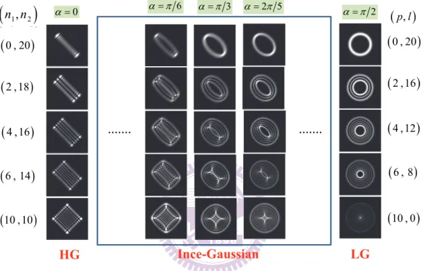
m m . Figure 2.1.1 and Fig. 2.1.2 depict the intensity distribution of n n1, 2 Hˆ for various indices



n n and values of 1, 2





  . Figure 2.1.1 and Fig. 2.1.2 are shown with the ,



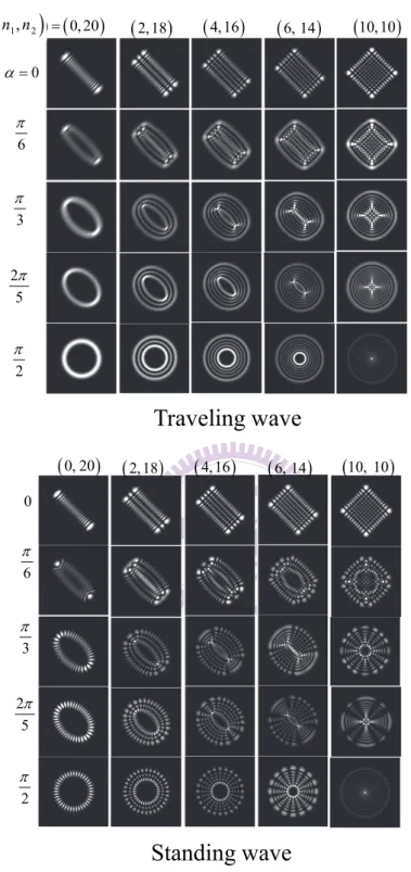
parameters   2 and   2 , respectively. It can be seen that the transformation from the HG to the LG modes can be continuously obtained by changing the parameter  or , which suggests different extent of coupling effect. The intermediate states, the Ince-Gaussian modes, are accessibly acquired through the SU(2) algebra associated with the coupled isotropic HO. Notably, the LG modes presented in Fig. 2.1.2(e) and Fig. 2.1.2(e’) possess fairly large orbital angular momentum per photon [19,20] of l5 and l52, respectively. Since light beams with well-defined orbital angular momentum have a number of developing applications [19,20], generation of such optical beams should be an important issue for further studies. Moreover, in Fig. 2.1.3, we present the comparison between the traveling-wave and the standing-wave forms of the eigenstates n n1, 2 Hˆ for

2

  . The standing-wave forms are obtained by taking the real part of the eigenstates n n1, 2 _Hˆ .

2.1.2 Coherent States : Single Periodic Orbits

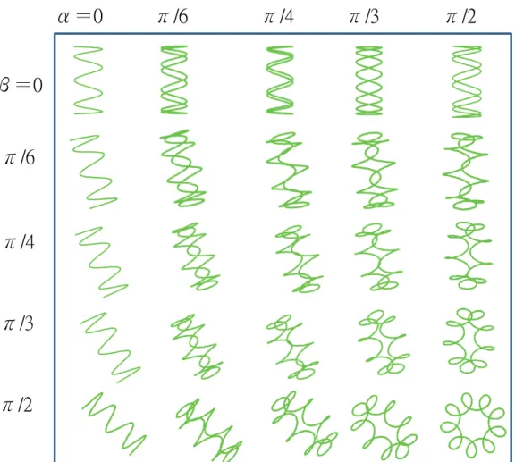
According to Eq. (2.1.8), we can obtain the classical orbits for Hˆ with the parametric equations x t( ) Re _v t₁

 

_ and y t( ) Re _v t₂

 

_, where

0     6   3 2 5   2



0 , 20





2 , 18





4 , 16





6 , 14





10 , 10



... ... HG Ince-Gaussian LG



m m1, 2





0 , 20





2 ,16





4 ,12





6 , 8





10 , 0



 

p l,



n n1, 2



Fig. 2.1.1 The intensity distribution of the eigenstates n n1, 2 Hˆ with different indices

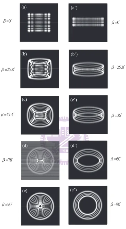
(a) (c) (e) (b) (d) β=0° β=47.4° β=90° β=25.8° β=78° β=0° β=36° β=90° β=60° β=25.8° (a’) (c’) (e’) (b’) (d’)

Fig. 2.1.2 The intensity distribution of the eigenstates n n1, 2 Hˆ with different indices



n n1, 2



, various values of  and constant value of   2 : (a)-(e)



n n1, 2







15,10



, (a’)-(e’)



n n1, 2







55,3



.