國 立 交 通 大 學
電機與控制工程學系
碩 士 論 文
利用虛擬實境駕駛模擬進行動態刺激下之
腦波反應研究
EEG Activities Related to Kinesthetic Stimuli in
Virtual Reality Simulated Dynamic Driving
研 究 生: 蕭 力 碩
指導教授: 林 進 燈 教授
利用虛擬實境駕駛模擬進行動態刺激下之
腦波反應研究
EEG Activities Related to Kinesthetic Stimuli in Virtual Reality
Simulated Dynamic Driving
研 究 生:蕭力碩 Student:
Li-Sor Hsiao
指導教授:林進燈 博士
Advisor:Dr. Chin-Teng Lin
國立交通大學
電機與控制工程學系
碩士論文
A Thesis
Submitted to Department of Electrical and Control Engineering
College of Engineering and Computer Science
National Chiao Tung University
in Partial Fulfillment of the Requirements
for the Degree of Master
in
Electrical and Control Engineering
June 2006
Hsinchu, Taiwan, Republic of China
利用虛擬實境駕駛模擬進行動態刺激下之
腦波反應研究
學生:蕭力碩
指導教授:林進燈 博士
國立交通大學電機與控制工程研究所
Chinese Abstract中文摘要
本論文以腦電波(Electroencephalogram, EEG)研究駕車動態刺激下之人類認知反 應,為研究特定行車事件下之人類認知狀態,研究中使用基於虛擬實境技術之動態駕車 模擬裝置來建立一逼真之駕車環境及駕車事件,包括在公路上的車輛加速、減速及偏 移。駕車模擬裝置中使用液壓六軸動態平臺提供駕駛員的動態感覺,此平臺依照車輛不 同方向的加速度變化會做出相對的傾斜動作。為了找出動態刺激對認知狀態之影響,我 們比較平臺開啟/關閉兩種狀態下受測者的 EEG 訊號來研究動態刺激對認知狀態的影響。 首先,EEG 訊號經過獨立成份分析(Independent Component Analysis, ICA)後分離成數 個獨立的訊號源。結果顯示出在運動皮質區有獨立之成份,並且與加減速行車動態相關 之 Alpha 頻帶 (8~12Hz) 能量抑制,並且在不同次實驗之間有很高的一致性。而在動 態偏移事件中,我們發現在大腦中心線 (Central Midline) 位置有負電位的產生。所 發現的大腦動態結果在不同受測者之間表現出重複的特性。本論文以事件相關電位 (Event Related Potential) 及 事 件 相 關 頻 譜 擾 動 (Event Related Spectral Perturbation)觀察腦動態,並首次發現可辨認、不同類動態刺激相關之腦電波。實驗 結果幫助我們更了解與動態感知相關的腦神經網路,也奠定了動態刺激與腦電波之相關 性研究一個重要基礎。EEG Activities Related to Kinesthetic Stimuli in
Virtual Reality Simulated Dynamic Driving
Student: Li-Sor Hsiao
Advisor: Dr. Chin-Teng Lin
Department of Electrical and Control Engineering
National Chiao Tung University
English Abstract
Abstract
The purpose of this study is to investigate Electroencephalography (EEG) dynamics in response to kinesthetic stimuli during driving. To study human cognition under specific driving task, we used Virtual Reality (VR) based driving simulator to create practical driving events; including acceleration, deceleration and deviation. The driving simulator includes Hydraulic Hexapod Motion Platform that provides tilt mechanism (to give roll, yaw, etc.) to simulate vehicle movement. In this study, we compare the EEG dynamics in response to kinesthetic stimulus while the platform is in action, compared to that were recorded when the platform is stationary. The scalp-recorded EEG channel signals were first separated into independent brain sources by Independent Component Analysis (ICA), then analyzed in time and frequency domains. Our results showed that independent component processes near the somatomotor cortex exhibited alpha power decreases that were consistent across sessions within subjects. Negative potential phase-locked to deviation events under motion condition was observed in a midline central component, which was consisted with the finding in the literature. The brain dynamics appears reproducible across sessions and subjects. This thesis, for the first time in the literature, reports distinctive brain dynamics measured by Event-Related-Potentials (ERP) and Event-Related-Spectral-Perturbations (ERSP) in response
to kinesthetic inputs of different types. The results help us to better understand different brain networks involving in driving and provide a foundation in studying EEG activities related to kinesthetic stimuli.
Keyword: Kinesthetic Stimulus, EEG, ICA, Component Clustering, ERSP, ERP, Mu Rhythm, EMG Chinese Acknowledgements
誌 謝
Acknowledgement 本論文的完成,首先要感謝我的指導教授 林進燈博士在過去兩年研究期間,提供 豐富的研究資源和實驗環境,並從旁指導協助,使得本文得以順利完成。 其次,我要感謝我的父母對我的照顧與栽培,教導我做人品德為最,強調人格健全 之發展與學習生活之態度,由於他們辛勞的付出和細心的照顧,才有今天的我。 特別感謝美國加州聖地牙哥大學的 鐘子平教授、 段正仁教授及 黃瑞松學長,給 予我研究上最大的協助,從實驗設計、實驗分析、實驗結果討論到論文撰寫,給我最專 業的意見跟看法。 另外,我要感謝腦科學研究實驗室的全體成員,沒有他們也就沒有我個人的成就。 特別感謝 梁勝富教授、蕭富仁教授、林文杰教授給予我在各方面的指導,無論是研究 上疑難的解答、研究方法、寫作方式、經驗分享等惠我良多。另外要感謝弘義、宗哲、 庭瑋同學,在過去兩年研究生活中同甘共苦,相互扶持。此外,我也要感謝陳玉潔學姊、 柯立偉學長與黃騰毅學長在研究上的幫助,還有感謝明達、弘章、林玫以及俊傑學弟妹, 在過去這一年中的相伴,以及碩士班新生青輔、尚文、孟修、依伶、德正在過去一個多 月的協助。同樣地也感謝實驗室助理在許多事務上的幫忙。 最後,我要感謝我的女朋友王郁喬小姐,替我分擔許多研究上的壓力與挫折,也讓 我在研究所的生活當中,增添更多色彩。 謹以本文獻給我親愛的家人與親友們,以及關心我的師長,願你們共享這份榮耀與 喜悅。Contents
Chinese Abstract...i
English Abstract ...ii
Acknowledgement...iv
Contents... v
Figures ...vii
Tables...ix
I. Introduction... 1
1.1. Vestibular system and kinesthetic stimulus response ...1
1.2. Kinesthetic perception during driving ...5
1.3. EEG studies under VR based dynamic driving ...6
1.4. Motivations and goal of this thesis...7
II. Material ... 9
2.1. Dynamic driving environment...10
2.1.1. VR scene...10
2.1.2. Hydraulic Hexapod Motion Platform...12
2.2. Introduction to motion tracking device ...14
2.3. EEG and EMG acquisition ...16
2.4. Subjects...18
III. Experimental Setup ... 19
3.1. Driving Experiment Event...19
3.2. Motion Profile ...22
IV. Data Analysis Procedure ... 23
4.1. Independent Component Analysis ...23
4.2. ERP Analysis ...27
4.3. ERSP Analysis...28
4.4. Component Clustering...31
4.4.1. The typical flow of clustering...32
4.4.2. Practical clustering ...34
V. Results... 36
5.1. Brain sources of kinesthetic stimulus response ...37
5.2. Within subject consistency ...42
5.3. Cross subject consistency ...48
VI. Discussion... 62
6.1. Mu Components ...62
6.3. Central midline components...66
6.4. Independent components not related to kinesthetic simuli...69
VII. Conclusion ... 70
Figures
Figure 1-1: The human vestibular system and anatomic identifications [41]. ...1 Figure 1-2: The ERP response to vertical Z axis rotation and acceleration. (a) ERP response to vertical Z axis rotation. 10,000°/sec2, 2 ms. (b) ERP response to vertical Z axis acceleration. 0.4g, 30 ms. ...3 Figure 1-3: The ERP response to X axis rotation. Upper plot: The rotation ERP under 1-G
gravity; Lower plot: The rotation ERP under 0-G gravity...4 Figure 2-1: The dynamic VR driving environment with physiological measurement system. ..9 Figure 2-2: The dynamic VR driving environment, Brain Research Center, National Chiao
Tung University, Taiwan, ROC ...10 Figure 2-3: The configuration of the 3D surrounded scene. The 3D VR scene consists of 7
projectors, creating a surrounded view. Frontal screen is overlapped by 2 projector frames in different polarizations, providing a stereoscopic VR scene for 3D visualization. ... 11 Figure 2-4: The overview of surrounded VR scene. The VR-based four-lane highway scenes
are projected into surround screen with seven projectors...12 Figure 2-5: The Stewart platform. (a) The sketch map for the Stewart platform. (b) The actual
Stewart platform. A driving cabin is mounted on this platform in our Lab...13 Figure 2-6: How motion platform works. http://www.force-dynamics.com/...13 Figure 2-7: The accelerometer or platform motion tracking, Inertia Sensing, InertiaCube 300
...15 Figure 2-8: The recording of orientation of InertiaCube2. (a) The demo program that shows
Pitch, Yaw and Roll recording. (b) The Roll, Pitch and Yaw axes. ...15 Figure 2-9: The International 10-20 system of electrode placement [43]. (a) lateral view. (b)
top view...16 Figure 2-10: The NuAmps EEG Amplifier and the Electrode Cap...17 Figure 3-1: The simulated high way scene. The visual information is reduced to minimum to
avoid unnecessary stimuli...19 Figure 3-2: Illustration of the design for stop-go event...20 Figure 3-3: Illustration of the deviation event. (a) Vehicle moving in straight line. (b)
Deviation event occurred. (c) Subject’s reaction. (d) Vehicle back to middle lane. ...21 Figure 4-1: Scalp topography of ICA decomposition...26 Figure 4-2: An ERP image includes the averaged ERP, response time and inter-trial
information. ...28 Figure 4-3: The data processing in ERSP analysis...30
Figure 4-5: A basic idea of component clustering. ...33
Figure 4-6: Component selection preceding clustering...34
Figure 4-7: Practical Clustering flowchart for our study...35
Figure 5-1 ICA decompositions and our interested components...38
Figure 5-2 The feature related to kinesthetic stimulus in stop-go events...39
Figure 5-3: ERSP group average of Mu components, deviation event. ...40
Figure 5-4: ERP group average of central midline component, deviation event...40
Figure 5-5: ERSP of S07-060321 COM12,...43
Figure 5-6: ERSP of S07-060322 COM10, Stop and Go event. ...44
Figure 5-7: ERSP of S07-060217 COM10, Stop and Go event. ...45
Figure 5-8: ERSP of S07-060321 COM09, Stop and Go event. ...46
Figure 5-9: ERP of S07-060217 COM03, Deviation event...47
Figure 5-10: ERP of S07-060322, Deviation event...47
Figure 5-11: ERSP of S03-050503 COM08, Stop and Go event. ...49
Figure 5-12: ERSP of S06-060215 COM06, Stop and Go event. ...50
Figure 5-13: ERP of S04-050509 COM02, Deviation event...51
Figure 5-14: ERP of S09-060315 COM03, Deviation event...51
Figure 5-15: Final Clustering result...53
Figure 5-16: Group Average of Left Mu Component...54
Figure 5-17: Group average of right Mu component. ...55
Figure 5-18: Group average of the central midline components...56
Figure 5-19: ERP reation time comparison. ...58
Figure 5-20: Left Mu ERSP of deviation events. ...59
Figure 5-21: Group average of occipital components. ...60
Figure 5-22: Group average of parietal components. ...61
Figure 5-23: Group average of frontal components. ...61
Figure 6-1: The electrode location of EMG signal...63
Figure 6-2: Go Event Neck EMG...64
Figure 6-3: Stop Event Neck EMG ...65
Tables
Table 2-1: The Specification of driving simulator...12
Table 2-2: NuAmps Specifications...18
Table 5-1: Subject list ...36
Table 5-2: Within-subject result of subject 7...42
Table 5-3 List of cross-subject analysis...48
Table 5-4: The experiment result table ...52
Table 5-5 List of response time in deviation. ...58
I. Introduction
The kinesthetic perception, the sensory apparatus that detects motions, is one of the most important sensations to human being, yet we usually overlook the contributions of vestibular system to our live, simply because it doesn’t give us the sense to this vivid and harmonic world like our eyes and ears do. Kinesthetic perception doesn’t taste or smell, making it less appreciated. However, we would not have a complete sensation without motion perception. If our vestibular system fails to perform, we would feel uncomfortable and/or even sick, for instance, the motion sickness. We cannot even stand still or walk in straight line without the vestibular system working properly. The vestibular system, thus, plays an important role in our life.
1.1. Vestibular system and kinesthetic stimulus response
Human vestibular system, a sensory apparatus locate bilaterally in the inners which detects the motion of the head and body in space [3]. It is composed of two functional parts shown as Figure 1-1: (1) the otolithic organs (blue and green colored areas), and (2) the
Figure 1-1: The human vestibular system and anatomic identifications [41]. Semicircular Canals Otolithic
semicircular canals (red, pink and orange areas). The otolithic organs detect linear accelerations [5][6][7], while the semicircular canals detect rotary accelerations [4].
Vestibular information has important roles in perceptual tasks such as ego-motion estimation [1]. In recent research, vestibular information was shown to disambiguate the interpretation of dynamic visual information during observer’s movement [2]. A complete investigation of either motion perception or vestibular system should include 6 Degree of Freedom (DOF), the movement in three linear axes: X-, Y-, and Z- axis, and rotations in all three rotary axes: pitch-, roll- and yaw-axis. So far very few papers had investigated all these 6 degree of movement. It is an extreme difficult task to study all kinds of movements, because of the lack of an appropriate platform to provide all 6 degrees of movements.
Researchers have tried to measure evoked potentials of vestibular origin for near 30 years. Three kinds of vestibular evoked potential (VESTEP) – short (<15ms), middle (15-30ms) and long (>30ms) latency brainstem potentials, defined by the duration of response, have been reported. The short latency potentials evoked by high angular acceleration impulses stimulating semicircular canals in humans [15][16][17][23] have been recorded. Elidan et al [15] reported the ERP response to high speed and short time vertical Z axis rotation. Subjects were rotated at speed of 10,000°/sec2 and duration of 2 ms Signals were measured from forehead mastoid electrode, negative peak at about 15 ms were observed, as shown in Figure 1-2(a). Baudonniere et al [25] showed the result of short (30 ms) linear displacements of subjects without co-stimulation of the semicircular canals evoked a biphasic negative wave, most prominent at midline central electrode (Cz) as shown in Figure 1-2(b).
(a) (b) Figure 1-2: The ERP response to vertical Z axis rotation and acceleration. (a) ERP response
to vertical Z axis rotation. 10,000°/sec2, 2 ms. (b) ERP response to vertical Z axis acceleration. 0.4g, 30 ms.
Long latency cortical potential evoked by stimulating horizontal semicircular canals with active head movements [26][27] and passive whole body movements [24][28][29] have been recorded. The VESTEP, evoked by stimulating otolithic and semicircular canals with different orientation of rotation or direction of movement was investigated in depth by Probst et al. [9][20][21][22]. One of their studies created microgravity condition by parabolic flight in order to avoid the co-stimulation of otolithic and semicircular canals. Figure 1-3 shows the ERP of rolling at X axis, bell-shaped negativity at midline central channel was recorded for roll up and down motion during microgravity.
Figure 1-3: The ERP response to X axis rotation. Upper plot: The rotation ERP under 1-G gravity; Lower plot: The rotation ERP under 0-G gravity
All aforementioned studies focused on the contribution of vestibular system, thus stimulus from visual and audio are completely isolated. Some studies [8] discussed about the perception to self-body movements, with participation of visual stimulation. Specialized motion platforms generated required body movements. Physiological acquisitions or questionnaire was used as a measurement to motion perception. Thilo et al., [8] used visual-evoked-potential (VEP) to compare the perception of object-motion and self-motion. They reported significant N70 amplitude difference in VEP when they compared perception
to “Static Body with Rotating Picture” and “Rotating Body with Static Picture.”
The experimental variables in these studies were well controlled, for instance, subjects were blindfolded VESTEP investigations [9][15] [25], or watching pixels moving or rotating on screen [8]. It might be desirable from the perspectives of scientific research, but less practical because we rarely experience vestibular stimulation without visual co-stimulation or watch pixels rotating or moving in a real world. We were actually living in a visual-vestibular co-stimulation world and the visual cue is always a meaningful and continuous scene, for instance, the driving motion.
1.2. Kinesthetic perception during driving
One of the most experienced kinesthetic perceptions in our life is the driving motion, in other word, the perception we sensed during the vehicle speed or direction change. Whenever the vehicle accelerates, decelerates or curves in a corner, we experience a force pulling our body against the direction of moving. For a driver, the perception to motion includes kinesthetic and visual stimulus. A driver does not sense only the pushing or pulling his/her body by a force, but also the scene change related to vehicle movement. The driving perception includes the co-stimulation of visual cue, vestibular stimulation, muscle reaction and skin pressure. It is indeed a complicated mechanism to understand.
There are numbers of difficulties in investigating the driving perception. First of all, the safety of subject must be guaranteed. Experiments should be held under a safe driving environment, it is very dangerous to conduct driving experiments on the road. Second, appropriate monitoring and data acquisition are needed to study the influence of kinesthetic stimuli. The stimulation should be simple enough and repeatable to keep experiment under control. Third, objective evaluation should be assessed in the studies.
is widely used in driving related researches [41]. For the necessity of motion during driving, literatures showed that the absence of motion information increased reaction times to external movement perturbations [32], and decreased safety margins in the control of lateral acceleration in curve driving [33]. In real driving, improper signals from disordered vestibular organs were reported to determine inappropriate steering adjustment [34]. Moreover, the presence of vestibular information in driving simulators shows the importance for it influences the perception of illusory self-tilt and illusory self-motion [35]. These studies emphasized the importance of motion perception during driving with the assessment of driving performance and behavior. Another research investigated how to duplicate the real driving motion to simulated driving [30]. However, assessing driving performance or behavior is not objective enough since the performance and behavior varies due to subject training or learning effect. In this thesis, we use a direct and objective method to evaluate human cognition during driving.
1.3. EEG studies under VR based dynamic driving
The electroencephalogram (EEG) has been used for 80 years in clinical paratices as well as basic scientific studies, it is a popular method for evaluating human cognition nowadays. It directly measures brain responses to external or internal stimulation. Much more information can be obtained from EEG compared to appearance behavior. Comparing to another widely used neuroimaging modality, functional Magnetic Resonance Imaging (fMRI), EEG is much less expensive and more portable, thus it is applicable in daily live, especially on the move.
In recent years, some researchers have designed the Virtual-Reality (VR) senses to provide appropriate environments for assessing brain activity during driving [68][70][72]. VR technology is gradually being recognized as a useful tool for the study and assessment of
VR environment combined with physiological and behavioral response recording offer more assessment options that are not available by traditional neuropsychological study approaches. The VR technique allows subjects to interact directly with a virtual environment rather than monotonic auditory and visual stimuli. It is an excellent strategy for brain research to provide interactive and realistic tasks due to low cost and preventing risks of operating actual vehicle in real environment. Integrating VR scenes with a dynamic motion platform, it is easier to study the brain activity response to kinesthetic stimulus. Therefore, the VR-based dynamic motion platform combined with EEG monitoring is an innovation in cognitive engineering research [68][69].
1.4. Motivations and goal of this thesis
The goal of this study is to assess the EEG dynamics in response to kinesthetic inputs during driving. To study human cognition under specific driving task we first construct a Virtual-Reality based interactive driving environment which integrates surrounded scene and hydraulic hexapod motion platform. The VR scene shows a vehicle driving on a 4-lane highway with high speed. A hexapod platform provides 6 DOF motion to simulate the dynamics in driving. This dynamic VR environment supports visual-vestibular co-stimulation for driving event. Using simple driving behavior such as deceleration, acceleration, and deviation, we study brain responses of kinesthetic input by comparing subjects’ EEG differences in motion and motionless conditions of dynamic platform. In the mean time, the posture of platform motion is recorded by an accelerometer, which allows us to observe the relationship between EEG response and platform motion. This thesis also provides a good evidence to show that the dynamic motion platform is required for the study of human cognitive state estimation under driving.
The thesis is organized in 7 chapters. Chapter 1 briefly introduces current knowledge in vestibular system and the goal of our study. Chapter 2 details the apparatus and materials of our study. Chapter 3 describes the details of experimental setup, including the time course of driving event and the platform motion setup. In chapter 4, we explore the EEG with innovative methods by combining Independent Component Analysis (ICA), time-frequency spectral analysis, ERP and component clustering. Chapter 5 shows the results. Chapter 6 discusses and compares our finding with previous studies, and finally we concluded in Chapter 7.
II. Material
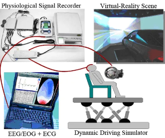
This chapter describes how a VR-based dynamic driving environment is designed and built up for interactive driving experiments. Figure 2-1 shows four major parts of the architecture: (1) a 3D highway driving scene based on the VR technology, (2) a real vehicle mounted on a 6-DOF motion platform, (3) a physiological signal measurement system with 36-channel EEG/EOG/ECG sensors, and (4) a signal processing module based on ICA decomposition, power spectral analysis and component clustering. The details of this environment will be presented as follows.
2.1. Dynamic driving environment
The dynamic driving environment provides a safe, time saving and low cost approach to study human cognition under realistic driving events. Our driving simulator provides not only high-fidelity VR scene, but also kinesthetic inputs and realistic driving environment (as shown in Figure 2-2). These make subjects feel that they are driving in a real vehicle on the real road.
Figure 2-2: The dynamic VR driving environment, Brain Research Center, National Chiao Tung University, Taiwan, ROC
2.1.1. VR scene
Our VR scene was developed by using the World Tool Kit (WTK) 3D engine. The 3D view was composed of seven identical PCs running the same VR program. Seven PCs were synchronized by LAN so all scenes were going at exactly same pace. The VR scenes of different viewpoints were projected on corresponding locations. Figure 2-3 shows the layout of our simulator. The front screen marked 1 and 2 was overlapped by two polarized frames to
frontal screen with two projectors, respectively. By wearing special glasses with a polarized filter, the configuration provides a stereoscopic VR scene for a 3D visualization.
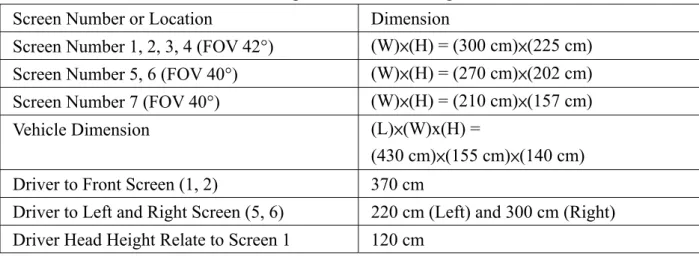
Literatures showed that the horizontal field of view (FOV) of 120° was needed for correct speed perception [31]. In our VR scene, the surrounded screens covered 206° frontal FOV and 40° back FOV, as shown in Figure 2-4. Frames projected from 7 projectors are connected side by side to construct a surrounded VR scene. The size of each screen has diagonal measuring 2.6-3.75 meters. The vehicle was placed at the center of the surrounded screens. Detailed information is shown in Table 2-1.
Figure 2-3: The configuration of the 3D surrounded scene. The 3D VR scene consists of 7 projectors, creating a surrounded view. Frontal screen is overlapped by 2 projector frames in different polarizations, providing a stereoscopic VR scene for 3D visualization.
2.1.2. Hydraulic Hexapod Motion Platform
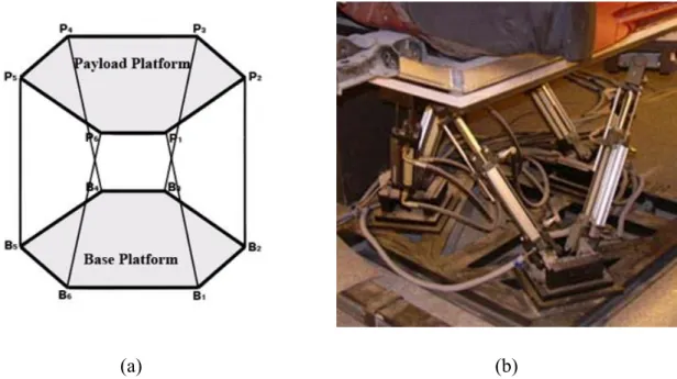
Several studies showed that vestibular cues have a role in speed control and steering [32][33]. The vestibular cues or the motion cues could be provided by a motion platform controlled by six hydraulic linear actuators. This hexapod configuration was also called Stewart Platform [36] (as shown in Figure 2-5). The platform generated accelerations in vertical, lateral and longitudinal direction of vehicle as well as pitch, roll and yaw angular
Table 2-1: The Specification of driving simulator
Screen Number or Location Dimension
Screen Number 1, 2, 3, 4 (FOV 42°) (W)×(H) = (300 cm)×(225 cm) Screen Number 5, 6 (FOV 40°) (W)×(H) = (270 cm)×(202 cm) Screen Number 7 (FOV 40°) (W)×(H) = (210 cm)×(157 cm)
Vehicle Dimension (L)×(W)x(H) =
(430 cm)×(155 cm)×(140 cm) Driver to Front Screen (1, 2) 370 cm
Driver to Left and Right Screen (5, 6) 220 cm (Left) and 300 cm (Right) Driver Head Height Relate to Screen 1 120 cm
Figure 2-4: The overview of surrounded VR scene. The VR-based four-lane highway scenes are projected into surround screen with seven projectors.
accelerations. Figure 2-6 shows a basic idea how the motion platform simulates driving
(a) (b)
Figure 2-5: The Stewart platform. (a) The sketch map for the Stewart platform. (b) The actual Stewart platform. A driving cabin is mounted on this platform in our Lab.
motion. When in deceleration, the driver feels a force pushes him/her against the belts, the platform tilts forward simultaneously to change the gravity direction sensed by the driver, and thus simulates the deceleration force. Similarly, the platform tilts backward to simulate acceleration force. This (or comparable) technique had been used widely in driving simulation studies [37].
The Hexapod Stewart Platform has superior performance in position control compared to traditional series manipulator. The parallel manipulator provides high-precision platform manipulations. Six extensible actuators equally share the loading of the platform, which provide high capability for realistic applications. Inverse kinematics analysis is used to solve the problem of converting the position and orientation of the payload platform with respect to the base platform. A singular solution of the inverse kinematics can be evaluated by simple formulae [38], which provides a high-speed platform and creats many possibilities for applications.
2.2. Introduction to motion tracking device
An accelerometer (inertia sensing, InertiaCube2 [39], as shown in Figure 2-7) was placed in the vehicle, at the center of movement. The InertiaCube2 is an inertial 3-DOF (Degree of Freedom) orientation tracking system. It obtains its motion sensing using a miniature solid-state inertial measurement unit, which senses angular rate of rotation, gravity and earth magnetic field along three perpendicular axes. The angular rates are integrated to obtain the orientations (yaw, pitch, and roll) of the sensors. Gravitometer and compass measurements are used to prevent the accumulation of gyroscopic drift. The InertiaCube2 is a monolithic part
based on micro-electro-mechanical systems (MEMS) technology involving no pinning wheels Figure 2-7: The accelerometer or platform motion tracking, Inertia Sensing, InertiaCube 300
(a) (b) Figure 2-8: The recording of orientation of InertiaCube2. (a) The demo program that shows
that might generate noise, inertial forces and mechanical failures [40]. InertiaCube2 transfers digital data using RS232 protocol and converts it to USB with a small converter box. This accelerometer records orientations of the vehicle in pitch, roll and yaw during driving simulation, as shown in Figure 2-8. We will analyze physiological data and the orientation recording to investigate the relationship between human cognition and kinesthetic stimulus.
2.3. EEG and EMG acquisition
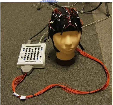
Subjects wore a movement-proof electrode cap with 36 sintered Ag/AgCl electrodes to measure the electrical activities of brain, i.e., EEG. The EEG electrodes were placed according to the international 10-20 system (as shown in Figure 2-9) with a unipolar reference at the right earlobe.
(a) (b) Figure 2-9: The International 10-20 system of electrode placement [43]. (a) lateral view.
The impedance between EEG electrodes and skin was kept to less than 5kΩ by injecting NaCl based conductive gel. Data were amplified and recorded by the Scan NuAmps Express system (Compumedics Ltd., VIC, Australia) shown in Figure 2-10, a high-quality 40-channel digital EEG amplifier capable of 32-bit precision sampled at 1000 Hz. Table 2-2 shows the specifications of the NuAmps amplifier. The EEG data were recorded with 16-bit quantization levels at a sampling rate of 500 Hz in this study.
Data were preprocessed using a low-pass filter with a cut-off frequency of 50 Hz in order to remove the power line noise and other high-frequency noise. Similarly, a high-pass filter with a cut-off frequency at 0.5 Hz was applied to remove baseline drifts.
2.4. Subjects
The purpose of this study is to investigate the subject brain responses to kinesthetic stimulus. The subjects were instructed to perform the driving task consciously. Statistical results showed that the drowsiest period occurs from late night to early morning, and during the early afternoon hours [42]. According to these results, the driving experiments were conducted in middle morning or late afternoon to avoid the drowsiest time.
Ten healthy subjects participated in this research (one female and eleven males, aged between 20 and 28). Subjects were instructed to keep the car at the center of the lane by controlling the steering wheel, and to perform the driving task consciously. Each subject completed four 25-minute sessions in each driving experiment. To prevent subjects from feeling drowsy during experiments, they rested for few minutes after each session until they were ready for the next one. The whole driving experiment lasted about 2 hours. Subjects performed at least 2 driving experiments on different days for verifying the cross-session consistency.
Table 2-2: NuAmps Specifications
Analog inputs 40 unipolar (bipolar derivations can be computed) Sampling frequencies 125, 250, 500, 1000 Hz per channel
Input Range ±130mV
Input Impedance Not less than 80 MOhm
Input noise 1 µV RMS (6 µV peak-to-peak)
Bandwidth 3dB down from DC to 262.5 Hz, dependent upon sampling frequency selected
III. Experimental Setup
To investigate the influence of driving kinesthetic stimulus on cognitive states, we designed three simple driving events: deceleration, acceleration and deviation. The 6-DOF motion platform provided corresponding movements for different driving events. By switching the platform between “motion mode” and “motionless mode”, we produced two identical driving conditions with the only difference of the presence of platform motion. The EEG signals were recorded, analyzed and compared under these two conditions.
3.1. Driving Experiment Event
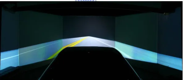
Figure 3-1: The simulated high way scene. The visual information is reduced to minimum to avoid unnecessary stimuli.
We developed a VR highway environment with a monotonic scene as shown in Figure 3-1 and eliminated all unnecessary visual stimuli. In the VR scene, the simulated driving speed was controlled by a scheduled program, thus subjects needed not to step on paddles, to prevent large muscle activity on the throttle or brake. We designed three driving events: stop,
go and deviation event. The stop and go events are paired, which means go event always follow the stop event, so we defined stop and go events as Stop-Go event. The deceleration and acceleration in Stop-Go event was controlled by a program. Figure 3-2 shows the time course of a Stop-Go event. If we define beginning of stop event as 0 second (bold arrow in Figure 3-2), a yellow light cue was shown on screen 1 second prior to the stop event. When a stop event began, the yellow light was replaced with a red light in same position, and the deceleration began. The car then slowed down and completely stopped in 4 seconds, the red light out. Stop lasted 7 seconds, and then the go event began. A green light was shown on screen, and start accelerating for 3 second. Then the green light was out, the vehicle was moving at constant speed, and a Stop-Go event ended.
During the experiment, subjects did not need to do anything in the stop and go events, but subjects were asked to handle the wheel to keep the car position at the center of cruising lane. During the experiment, the vehicle were randomly drifted away the crusing position, and the subjects were instructed to steer the vehicle back to the center of the crusing lane as
moment the subject first steered the wheel to compensate the drift, were recorded for further analysis.
Figure 3-3 illustrates a deviation event. In phase 1 (Figure 3-3a), vehicle was moving forward in a straight line. Deviation event first occurred at the beginning of Phase 2 (Figure 3-3b), in which the vehicle deviated from the original cruising position. The vehicle deviated either to left or right. The deviation event enters Phase 3 when the subject started steering the vehicle back to the cruising position (Figure 3-3c). The subject would continue to steer the car until s/he thinks the car has returned to the center of the cruising lane. The moment of subject stopped the steering effort marked the beginning of the Phase 4 of the drift event (Figure 3-3d). The inter-event interval is 9 seconds. The Stop-Go event and deviation event were randomly occurred with the probability of 50%.
(a) (b) (c) (d) Figure 3-3: Illustration of the deviation event. (a) Vehicle moving in straight line. (b)
Deviation event occurred. (c) Subject’s reaction. (d) Vehicle back to middle lane.
Response time was recorded
3.2. Motion Profile
The experiment includes two conditions, the “motion mode” and “motionless mode”. This was achieved by enabling or disabling the motion platform action. The platform motion in “motion session” was recorded through accelerometer as shown in Figure 3-2. The platform performed a pitching forward action in a stop-event, the angle was nearly 5 degrees, and a pitching backward action was performed in a go-event, the angle was nearly 4 degrees. With these movements, subjects felt forward force while decelerating, backward force while accelerating and a sudden shaking while deviating due to the platform position change. In the “motionless session” the platform was static and not response to the speed change or deviation of vehicle, only visually event was presented to driver. Each subject completed 4 sessions in a driving experiment, sessions were motion and motionless counterbalanced and each lasted 25 minutes. After each session subjects took a 5-10 min rest to prevent the drowsiness in driving. In order to confirm the consistency of subject’s brain activities from different experiments, each subjects completed 2~4 driving experiments for within-subject analysis.
IV. Data Analysis Procedure
In this study, the mutli-channel EEG signals were first separated into independent brain sources using Independent Component Analysis (ICA) [71]. Then we ploted the separated signals using Event Related Spectral Perturbation (ERSP) plot developed by Makeig, 1993 [61] and Event Related Potential (ERP). We then investigated the stability of component activations and scalp topographies of meaningful components across sessions within each subject. To test the reproducibility of component maps and activations across subjects, we performed component clustering analysis (detailed below).
4.1. Independent Component Analysis
The joint problems of electroencephalographic (EEG) source segregation, identification, and localization are very difficult since the EEG data collected from any point on the human scalp includes activity generated within a large brain area. The problem of determining brain electrical sources from potential patterns recorded on the scalp surface is mathematically underdetermined. Although the conductivity between the skull and brain is different, the spatial smearing of EEG data by volume conduction does not cause significant time delay and it suggests that the ICA algorithm is suitable for performing blind source separation on EEG data. The ICA methods were extensively applied to blind source separation problem since 1990s [45]-[52]. In recent years, subsequent technical reports [53]-[60] demonstrated that ICA was a suitable solution to the problem of EEG source segregation, identification, and localization based on the following assumptions: (1) The conduction of the EEG sensors is instantaneous and linear such that the measured mixing signals are linear and the propagation delays are negligible. (2) The signal source of muscle activity, eye, and, cardiac signals are
not time locked to the sources of EEG activity which is regarded as reflecting synaptic activity of cortical neurons [53][54].
In this study, we attempt to completely separate the twin problems of source identification and source localization by using a generally applicable ICA. Thus, the artifacts including the eye-movement (EOG), eye-blinking, heart-beating (EKG), muscle-movement (EMG), and line noises can be successfully separated from EEG activities. The ICA is a statistical “latent variables” model with generative form:
) t ( ) t ( As x = (1)
where A is a linear transform called a mixing matrix and the s are statistically mutually i independent. The ICA model describes how the observed data are generated by a process of mixing the components s . The independent components i s (often abbreviated as ICs) are i latent variables, meaning that they cannot be directly observed. Also the mixing matrix A is assumed to be unknown. All we observed are the random variables x , and we must estimate i both the mixing matrix and the IC’s s using the i x . i
Therefore, given time series of the observed data
[
]
T N(t) x ) t ( x ) t ( x ) t ( = 1 2 L x inN-dimension, ICA will find a linear mapping W such that the unmixed signals u(t) are
statically independent. ) t ( ) t ( Wx u = . (2)
Supposed the probability density function of the observations x can be expressed as:
) ( p ) det( ) ( p x = W u , (3)
the learning algorithm can be derived using the maximum likelihood formulation with the log-likelihood function derived as:
∑
+=logdet( ) N logpi(ui)
) ,
(uW W
Thus, an effective learning algorithm using natural gradient to maximize the log-likelihood with respect to W gives:
[
I u u]
W W W W W u W L( , ) T ϕ( ) T Δ = − ∂ ∂ ∝ , (5)where the nonlinearity
T N u ) u ( p u ) u ( p ) ( p ) u ( p ) u ( p ) ( p ) ( N N ⎥ ⎥ ⎦ ⎤ ⎢ ⎢ ⎣ ⎡ − − = − = ∂ ∂ ∂ ∂ ∂ ∂ L 1 1 1 u u u u ϕ , (6)
and WTW rescales the gradient, simplifies the learning rule and speeds the convergence
considerably. It is difficult to know a priori the parametric density function p u , which ( )
plays an essential role in the learning process. If we choose to approximate the estimated probability density function with an Edgeworth expansion or Gram-Charlier expansion for generalizing the learning rule to sources with either sub- or super-Gaussian distributions, the nonlinearity ϕ( u) can be derived as:
⎩ ⎨ ⎧ + − = sources, gaussian -sub for : ) tanh( sources, gaussian -super for : ) tanh( ) ( u u u u u ϕ (7) Then,
[
]
[
]
⎩ ⎨ ⎧ − + − − = Δ gaussian, -sub : ) tanh( gaussian, -super : ) tanh( W uu u u I W uu u u I T T T T W (8)Since there is no general definition for sub- and super-Gaussian sources, we choose
(
(1,1) (-1,1))
2
1 N N
) (
p u = + and p(u)=N(0,1)sech2(u) for sub- and super-Gaussian,
respectively, where
(
μ σ2)
,
N is a normal distribution. The learning rules differ in the sign
before the tanh function and can be determined using a switching criterion as:
[
]
⎩ ⎨ ⎧ − = = − − ∝ Δ gaussian, -sub : 1 gaussian, -super : 1 where , ) tanh( i i κ κ W uu u u K I W T T (9)where
{
} { }
{
}
(
sec 2( ) 2 tanh( ))
, i i i i i =signE h u Eu −E u u κ (10)represents the elements of N-dimensional diagonal matrix K. After ICA training, we can obtain N ICA components u(t) decomposed from the measured N-channel EEG data x(t). In this study, N=30, thus we obtain 30 components from 30 channel signals.
). ( ) ( ) ( ) ( ) ( ) ( ) ( ) ( 33 33 , 33 33 , 2 33 , 1 2 2 , 33 2 , 2 2 , 1 1 1 , 33 1 , 2 1 , 1 33 2 1 t u w w w t u w w w t u w w w t t x t x t x t ⎥ ⎥ ⎥ ⎥ ⎦ ⎤ ⎢ ⎢ ⎢ ⎢ ⎣ ⎡ + + ⎥ ⎥ ⎥ ⎥ ⎦ ⎤ ⎢ ⎢ ⎢ ⎢ ⎣ ⎡ + ⎥ ⎥ ⎥ ⎥ ⎦ ⎤ ⎢ ⎢ ⎢ ⎢ ⎣ ⎡ = = ⎥ ⎥ ⎥ ⎥ ⎦ ⎤ ⎢ ⎢ ⎢ ⎢ ⎣ ⎡ = M L M M M Wu x (11)
Figure 4-1 shows a result of the scalp topographies of ICA weighting matrix W corresponding to each ICA component by projecting each component onto the surface of the scalp, which provide evidence for the components' physiological origins, e.g., eye activity
was projected mainly to frontal sites, and the drowsiness-related potential is on the parietal lobe and occipital lobe [68], motor related potential will locate at left and right side of front parietal lobe, etc. We can see that most of artifacts and channel noises are effectively separated into independent components 1 and 3.
4.2. ERP Analysis
Dawson first recorded the evoked potentials (EP) from cerebral cortex by taking pictures and accumulation skill in 1947 [73]. Dawson initiated the new field of neuro-physiology by introducing the technology of averaging evoked potentials (AEP) in 1951. The AEP technology is extensively applied to many experiments which relate to specific stimulus event, and is named event-related potentials (ERP) in recent years. The narrow definition of ERP is to present a specific region of perceptual systems and elicit potential changes on the cerebral cortex when the stimulus appears or disappears. The board definition of ERP suggests the responses come from all parts of neural system.
Generally, the ERP induced by the stimulus is 2 ~ 10 μV, much smaller than the amplitudes of ongoing EEG, and it is thus often buried in the EEG recordings. EEG signals are composed of small signals and big noise. In order to extract the ERP from EEG signal, we need to increase the signal to noise ratio by presenting the same type of stimuli to the subject repeatedly. ERP is often obtained by averaging EEG signals of accumulated single trials of the same condition. Ongoing EEG signals across single trials are considered random and independent of the stimulus. However, it is assumed that the waveform and latency of ERP pattern are invariant to the same stimulus. Through phase cancellation, time- and phase locked EEG signals will be more prominent. For example, if the number of trials for condition is n, the ERP will be n times the amplitude of original wave pattern and the EEG amplitude will only be n times of the initial signal. Therefore, the signal to noise ratio (SNR) will be
improved by n times. Therefore, ERP sometimes can be named Averaged Evoked Potentials and this is the basic theorem of extracting the ERP [44].
Figure 4-2: An ERP image includes the averaged ERP, response time and inter-trial information.
4.3. ERSP Analysis
The Event Related Spectral Perturbation, or ERSP, was first proposed by Makeig [61]. The ERSP reveals aspects of event-related brain dynamics not contained in the ERP average of the same response epochs. The limitation of ERP is that it must be coherent time-and-phase-locked activities. Averaging same response epochs would involve phase cancellation, brain activities not exactly synchronized in both time and phase are averaged out. The ERSP measures average dynamic changes in amplitudes of the broad band EEG spectrum as a function of time following cognitive events. Through ERSP, we are able to observe time-locked but not necessary phase-lock activities.
The processing flow is shown in Figure 4-2. The time sequence of EEG channel data or ICA activations are subject to Fast Fourier Transform (FFT) with overlapped moving
windows. Spectrums prior to event onsets are considered as baseline spectra. The mean baseline spectra were converted into dB power and subtracted from spectral power after stimulus onsets so that we can visualize spectral ‘perturbation’ from the baseline. To reduce random error, spectrums in each epoch were smoothed by 3-windows moving-average. This procedure is applied to all the epochs, the results are then averaged to yield ERSP image.
The ERSP image mainly shows spectral differences after event, since the baseline spectra prior to event onsets have been removed. For instance, in the bottom of Figure 4-2 we can see very clearly that only little or no changes in high frequency band (the lower position the higher frequency) but very significant changes in low frequency band after event. This allows us to visualize spectral power change related to event.
After performing bootstrap analysis (usually 0.01 or 0.03, here we use 0.01) on ERSP, only statistically significant (p<0.01) spectral changes will be shown in the ERSP images. Non-significant time/frequency points are masked (replaced with zero). Any perturbations in frequency domain become relatively prominent.
While the ERSP reveals new and potentially important information about event-related brain dynamics, it cannot reveal interactions between the ERP amplitude, latency variability, and EEG spectral modulation. Figure 4-4 shows the ERSP of deviation event in motion and motionless conditions, and the limitation of ERSP. We can’t find obvious difference related to kinesthetic stimulus. In contrast, the ERP (the bottom of Figure 4-4) showed very clear difference between two ERPs, a negative potential appear in motion-deviation but not in motionless-deviation. This example shows that ERSP and ERP are complimentary and should be take into account when we compare and contrast the brain responses across different conditions.
Figure 4-4: ERSP of deviation event on central midline. Figure 4-3: The data processing in ERSP analysis.
4.4. Component Clustering
To study the cross-subject component stability of ICA decomposition, components from multiple sessions and subjects were clustered based on their spatial distributions and EEG characteristics. The usual practice to analyze cross-subject consistency was to compare the components one by one. However, this was a time-consuming task and might not be objective enough since analyst chose similar components by his/her own decision. There is no natural and easy way to identify a component from one subject with one or more components from another subject. A pair of independent components from two subjects might resemble and/or differ from each other in many ways and to different degrees. Furthermore, there is rather a lot of inter-subject variability not only in gross brain anatomy, but in functional mapping (electrical). Independent component analysis might derive different mixing matrix that maps brain source activity to the scalp to alleviate the inter-subject anatomical variability. But, component activations might remain quite variable because of the inter-subject functional variability. Components from different subjects thus may differ in many ways such as scalp maps, power spectra, ERPs and ERSPs.
Westerfield, Makeig, Delorme and Onton et al [62][63][64] attempted to solve this problem by calculating the similarities (distance) among different independent components. Components from multiple subjects were clustered in terms of their scalp maps and activation power spectra. Individual component clusters were characterized by their mean cluster map and activity spectrum. This method was also known as component clustering.
4.4.1. The typical flow of clustering
Component Clustering divided massive components into several significant clusters (Figure 4-5), for instance, assuming we have 10 subjects each of which includes 30 components after ICA decomposition, results in totally 300 components. To cluster these components into small number (for instance, 10) of groups, one approach is to apply kmeans on their scalp map and power spectral. Before the classification we apply PCA on scalp map and power spectral sequences to reduce dimensionality of the data. The kmeans algorithm measures the distance of every component pair and groups components into clusters. Ideally, components in the same cluster would have similar scalp map and power spectral characteristics, as shown in the bottom of Figure 4-5.
In practice, we can hardly achieve such clean clusters as in Figure 4-5 if we rely entirely on kmeans to classify components, since less then half of components were meaningful after ICA decomposition, others were usually account for noises. These components might confuse kmeans algorithm and reduce the consistency of each clusters. Another problem arises from combining scalp map and power spectral information for kmean classification. It remains an open question how to weight the spatial information (scalp maps) and source activity, accounted for by power spectra in the kmeans clustering. Below we propose a two-step clustering method.
4.4.2. Practical clustering
In previous session we mentioned 2 critical problems while applying typical kmean clustering. The first problem is the large number of ‘noisy’ components from ICA, making kmeans unable to group meaningful components together. This can be solved by selecting good components before kmeans. As shown in Figure 4-6, in ICA decompositions, half of them are considered as noisy components. These noisy components are removed from any further analysis.
Another problem is how to concatenate scalp map and power spectral information. We purpose to modify the typical classification (Figure 4-5) into a 2-stage clustering method (Figure 4-7) to solve this problem. The 2 stage clustering is to apply kmean twice, first stage classifies scalp map and second stage classifies power spectral. The first kmeans guarantees consistent anatomic features within the same cluster, and second kmeans guarantees consistent within-cluster functionality, characterized by power spectra.
Figure 4-7 shows our clustering flow. Components are first selected by observation and largely reduce to about half. Secondly, the selected components are classified by kmeans algorithm into 40 clusters in terms of component scalp maps (EEG.icawinv). Then we group 40 clusters into 10 significant clusters and discard some non-significant clusters manually. The resultant clusters are named according to the source locations of components. To uarantee the final results are with same functionality, we apply kmeans again on each of 10 significant clusters based on power spectra of the components. The second stage kmeans classifies components within some clusters into 4 sub-clusters. By observing the content of clusters we reject the minority one, which includes components with unwanted spectral, and group the remaining clusters. The resultant clusters have consistent anatomic and functional features.
V. Results
In the thesis we collect and analyze 31 driving experiments from 10 subjects, as listed in table 5-1, each subject completed 2~5 experiments. Each experiment includes 4 sessions and lasts 2 hours. Sessions are divided into ‘motion’ and ‘motionless’ sessions with stop, go and deviation events. Thus we have six conditions: “Motion-Stop”, “Motion-Go”, “Motion-Deviation”, “Motionless-Stop”, “Motionless-Go” and finally “Motionless-Deviation”. By comparing the motion & motionless pair, we may find some differences between these two conditions. Below we will first show our final result and then present detailed information of how we make the conclusion, starting from within-subject analysis, cross-subject analysis and finally component clusters.
Table 5-1: Subject list
Subject No. Exp.1 Exp.2 Exp.3 Exp.4 Exp.5
S03 05/04/27 05/04/29 05/05/03 05/05/10 S04 05/05/02 05/05/04 05/05/09 05/05/11 05/05/16 S05 05/05/17 05/06/03 05/06/07 05/06/10 S06 06/02/16 06/02/21 06/02/23 S07 06/02/17 06/03/21 06/03/22 S08 06/02/24 06/03/02 S09 06/02/24 06/03/09 06/03/15 S10 06/04/18 06/04/19 S11 06/04/20 06/04/21 S12 06/04/24 06/04/28 06/05/02
5.1. Brain sources of kinesthetic stimulus response
First of all, we compare the ERP or ERSP of the driving events in the two conditions: motion or motionless, to find some significant components. Figure 5-1 showed the components we are interested in, which were selected based on their characteristic scalp maps, dipole source locations, spectral signatures, and within subject consistency. Through detailed observation of 31 experiments results from 10 subjects, some localized components had been selected. The circled components in Figure 5-1, left Mu, right Mu and central midline components, show statistically significant response differences across conditions.
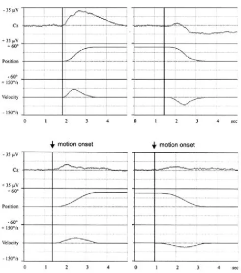
The ERP of the central midline component and the ERSPs of Mu components showed significant activity in response to kinesthetic stimulus. Figure 5-2 showed the result from stop-go events. ERSP images on the left are brain responses in “motion” conditions and the ones on the right are under “motionless” condition, respectively. The curves below the images are platform motion recordings (pitching, rotate by Y axis). We found Mu blocking time-locked to peak of platform motion in Stop-Motion and Go-Motion events, as shown in Figure 5-2a and 5-2b. In contrast, no Mu blocking occurred in Stop-Motionless and Go-Motionless events. Thus the Mu blocking is considered as brain responses to the kinesthetic input response of stop and go events. Figure 5-2c and 5-2d show the central midline component ERP image of stop-go events. Biphasic ERP peaks at 4000 ms after cue in stop event, similar ERPs can be found in go events, though it was not as clear as in stop events.
The deviation events showed similar results. Figure 5-3 shows the ERSP of left Mu components in deviation events. The curve below the ERSP shows the recorded platform motion, notice that the motion platform tilted along different directions in stop-go and deviation. In deviation events, platform rotated slightly along vertical Z axis. Since it was known that Mu been blocked whenever subject intended to move any part of his/her body.
The ERSP was dominated by Mu blockings in both motion and motionless conditions, resulted from subjects’ steering during deviation events. However, if we examine the ERSP carefully, we could find some differences between motion and motionless conditions. In particular, the Mu activity was blocked slightly earlier in motion-deviations, and the reaction time in motion-deviations was shorter than that in motionless-deviations. Figure 5-4 showed the central midline component ERP image and response time following deviation events. A negative ERP occurred in the central midline area, peaks at ~250 ms, which was very close to the beginning of the platform movement. The negativity is time-locked to deviation event and but not the response time. This negative ERP did not occurred in motionless condition. Thus, the negativity was primarily induced by the platform motion.
Figure 5-1 ICA decompositions and our interested components.
Central Midline
Left Mu
Right Mu
Motion Motionless
Figure 5-2 The feature related to kinesthetic stimulus in stop-go events.
(b) Go Event
(a) Stop Event
(c) Stop
Event
(d) Go
Event
Motion Motionless
Figure 5-3: ERSP group average of Mu components, deviation event.
Motion Motionless
From the ERP images in Figure 5-4 we can also see the response time of steering (the bold curve). The dashed curve in left side ERP indicated the response time in motionless deviations, thus we can easily compare the response time in two different conditions. It was evident that subject reacted faster in motion-deviation than in motionless-deviation.
We briefly concluded that, whenever a kinesthetic stimulus happened in driving, it induced Mu blocking (as shown in Figures 5-2a and 5-2b) and negative ERP in central midline component (as shown in Figures 5-2c, 5-2d, and 5-4). The presence of motion in driving also decreased response time (which was observed from deviation events). This will be discussed in detailed in the next chapter.
5.2. Within subject consistency
To test the reliability of experiment results, first we compare results of different experiments from the same subject in order to ensure the features are reproducable. The following 5 pages show the results from 2 experiments recorded on different days from Subject 7 for the stop , go and deviation events. Table 5-2 summarizes the findings.
In Figures 5-5, 5-6, 5-7 and 5-8, the scalp map, power spectral and dipole location are shown in upper half figure, ERSPs of 4 different conditions (motion-go, motion-stop, motionless-go and motionless-stop) and the platform motion recording are shown in lower half of the figure. The results show that alpha and beta band suppression time-locked to movement in the left and right Mu components, and are consistent across different sessions.
Figures 5-9 and 5-10 show the result of deviation event. Four ERP images in the figure represent deviate-left-motion, deviate-right-motion, deviate-left-motionless, and deviate-right- motionless. The platform motion recordings are shown below the ERP. Figures 5-9 and 5-10 show evident stimulus-locked negative potential following the deviation. The results are very consistent across session from the subject.
Table 5-2: Within-subject result of subject 7
Page Fig.NO Event Location Date Analysis
39 5-5 06/03/21 40 5-6 Right Mu 06/03/22 41 5-7 06/02/17 42 5-8 Stop-Go Left Mu 06/03/21
ERSPs show 10 & 20 Hz suppression time-locked to movement on left and right Mu components
43 5-9 06/02/17
43 5-10
Deviation Central
Midline 06/03/22
ERPs show stimulus-locked negative potential
Stop – Motion Stop – Motionless
Go – Motion Go – Motionless
Figure 5-5: ERSP of S07-060321 COM12, Stop and Go event.Stop – Motion Stop – Motionless
Go – Motion Go – Motionless
Figure 5-6: ERSP of S07-060322 COM10, Stop and Go event.Stop – Motion Stop – Motionless
Go – Motion Go – Motionless
Figure 5-7: ERSP of S07-060217 COM10, Stop and Go event.Stop – Motion Stop – Motionless
Go – Motion Go – Motionless
Figure 5-8: ERSP of S07-060321 COM09, Stop and Go event.Motion Motionless
Figure 5-9: ERP of S07-060217 COM03, Deviation event.
Motion Motionless
Figure 5-10: ERP of S07-060322, Deviation event.Deviation Left
Deviation Right
Deviation Left
5.3. Cross subject consistency
To examine the cross subject consistency of experiment results, we plot the results of subjects 3, 4, 6 and 9 in the next 3 pages in the events of stop, go and deviation. Table 5-3 summarizes the results of the figures.
In Figure 5-11 and 5-12, the scalp map, power spectral and dipole location are shown in upper half of the figure, ERSPs of 4 different conditions (motion-go, motion- stop, motionless-go and motionless-stop) and the platform motion recording are shown in lower half figure. The results show alpha band suppression time-locked to platform movement in right Mu components, which is consistent in subject 3 and subject 6.
Figure 5-13 and 5-14 show the result of deviation events. Four ERP images in the figure represent deviate-left-motion, deviate-right-motion, deviate-left-motionless, and deviate-right- motionless, respectively. The platform motion recordings are shown below the ERP plots. The figures show evident stimulus-locked negative potential which is very consistent in subjects 4 and 9.
Table 5-3 List of cross-subject analysis
Page Fig.NO Event Location Subject Analysis
45 5-11 S3
46 5-12
Stop-Go Right Mu
S6
ERSPs show alpha suppression time-locked to the platform movement
47 5-13 S4
47 5-14
Deviation Central Midline S9
ERP images show stimulus-locked negative potential in response to the platform movement.
Stop – Motion Stop – Motionless
Go – Motion Go – Motionless
Stop – Motion Stop – Motionless
Go – Motion Go – Motionless
Motion Motionless
Figure 5-13: ERP of S04-050509 COM02, Deviation event.Motion Motionless
Figure 5-14: ERP of S09-060315 COM03, Deviation event.Deviation Right
Deviation Right
Deviation Left
From these figures we find alpha suppression in stop and go events in Mu components of subject 3 and 6, and negative event-related potential stimulus-locked to deviation in central midline component of subjects 4 and 9. A more detailed result is shown in Table 5-4. In ten subjects, eight of them exhibit 10 or 10+20 Hz activity suppression in stop and go events, subjects 10 and 11 did not show any suppression in the motor cortex. It is very interesting that we observe power increase at 10~20 Hz in the stop event of subject 8 but power decrease in go event of same subject. Since this phenomenon is only found in subject 8 so we consider it as an outliner. Following deviation events, we fine negative ERP related to kinesthetic stimulus, in central midline component. These results show great consistency across nine of ten subjects participated in the study.
Table 5-4: The experiment result table
Subject
Stop
Go
Stop
Go
Deviation
S3 (4d) 10 Hz↓ 10&20↓ 10 ↓ 10&20 ↓ ERP
S4 (5d) 10 ↓ 10 ↓ 10 ↓ 10 ↓ ERP
S5 (4d) 10~20 ↓ 10~20 ↓ 10~20 ↓ 10~20 ↓ ERP
S6 (3d) 10 ↓ 10 ↓ 10 ↓ 10 ↓ ERP
S7 (3d) 10 ↓ 10&20 ↓ 10&20 ↓ 10&20 ↓ ERP
S8 (2d) 10~20 ↑ 10~20↓ 10~20 ↑ 10~20↓ ERP
S9 (3d) 10 ↓ 10 ↓ 10 ↓ 10 ↓ ERP
S10 (2d) ─ ─ ─ ─ ERP
S11 (2d) ─ ─ ─ ─ ─
S12 (3d) 10 ↓ 10 ↓ 10 ↓ 10 ↓ ERP
↓: power decrease in spectral ↑: power increase in spectral
5.4. Component Stability
From 10 subjects we collected a total of 930 components (30 components x 31 subjects) after ICA decomposition. The massive components are clustered into 10 largest non-artifactual clusters. The average scalp maps of these clusters are shown in Figure 5-15. Components in the same cluster have similar characteristics of scalp maps and power spectra.
Figure 5-15: Final Clustering result.
The group average ERSPs of left and right Mu Components are shown in Figures 5-16 and 5-17. Figure 5-16 shows the ERSPs of stop and go event averaged from 29 left Mu components. Similarly, Figure 5-17 shows the average of 32 right Mu components. Figure 5-18 shows the averaged ERP following deviation events of the central midline component cluster.
Average of 29 Components
Average Scalp Map
Average of 32 Components
Average Scalp Map
Average Scalp Map
![Figure 1-1: The human vestibular system and anatomic identifications [41]. Semicircular Canals Otolithic](https://thumb-ap.123doks.com/thumbv2/9libinfo/8251768.171729/12.892.155.775.548.912/figure-human-vestibular-anatomic-identifications-semicircular-canals-otolithic.webp)