Fast parking control of mobile robots: A motion planning approach with experimental validation

Fast Parking Control of Mobile Robots: A Motion

Planning Approach With Experimental Validation

Ti-Chung Lee, Chi-Yi Tsai, and Kai-Tai Song, Associate Member, IEEE

Abstract—This paper presents a solution to the general parking problem of nonholonomic mobile robots based on motion planning and tracking controller design. A new global tracking controller is first proposed to achieve global uniformly asymptotic stability and local exponential convergence. The parking problem is then transformed into a tracking one by adding a redesigned virtual trajectory to the original trajectory, thus guaranteeing practical stability with exponential convergence. Further improvement in parking performance is obtained through linearization and pole-placement methods. One feature of our approach is that fast convergence in parking and tracking can be treated at the same time without switching between two controllers. Moreover, a tuning function is used to enhance parking performance. With the proposed framework, various tracking controllers given in the literature can be adopted to handle parking problems. The effec-tiveness of the proposed methods is verified by several interesting experiments including parallel parking and back-into-garage parking.

Index Terms—Locally exponential convergence, mobile robots, motion planning, parking control, pole placement, tracking control.

I. INTRODUCTION

M

OBILE robot tracking control problems have been studied extensively in recent decades [15], [20], [21], [34]. Reported controllers are usually simple and can achieve fast tracking control. In general, getting a nonholonomic mobile robot to track a moving trajectory (the tracking problem) is often easier than getting it to stop at a specified location (the parking problem) [26]. In fact, it is well known that according to Brockett’s theorem [3], [30], the parking problem cannot be solved by employing continuous time-invariant feedback. To overcome this shortcoming and solve the regulation (parking) problem for general nonholonomic systems, including uni-cycle-modeled mobile robots, several research directions have been tried using nonlinear control approaches [1], [2], [4]–[7], [9]–[13], [17], [18], [21]–[25], [29], [30], [32], [33], [36]. For detailed discussions and comments on recent developments, see [21].

Manuscript received February 21, 2003; revised November 6, 2003. Manuscript received in final form January 14, 2004. Recommended by Associate Editor K. Moore. This work was supported by the National Science Council of Taiwan, R.O.C., under Grants NSC 90-2213-E-009-023, NSC 90-2213-E-009-027, and NSC-91-2213-E-159-004.

T.-C. Lee is with the Department of Electrical Engineering, Ming Hsin University of Science and Technology, Hsinchu 304, Taiwan, R.O.C. (e-mail: tc1120@ ms19.hinet.net).

C.-Y. Tsai and K.-T. Song are with the Department of Electrical and Con-trol Engineering, National Chiao Tung University, Hsinchu 300, Taiwan, R.O.C. (e-mail: [email protected]; [email protected]).

Digital Object Identifier 10.1109/TCST.2004.826964

Recently, research interest has centered on improving tracking performance, especially in the areas of convergence rate and robustness. It is well known that smooth feedback cannot achieve an exponential convergence rate [23]. Thus, most of the exponential stabilizers in the current literature employ either discontinuous feedback laws [1] or continuous but not differentiable functions [6], [23], [24], [36]. Another approach adopts some kind of linearization technique to guarantee exponential convergence to within any desired small radius of the origin [4], [18]. In [22], an interesting example was proposed to show that although the continuous homoge-neous feedback laws proposed in recent literature can achieve exponential convergence, they are not robust w.r.t. system uncertainty in general. Because of this, problems concerning robust control have recently attracted much research attention [13], [14], [18].

Despite the apparent advances represented by the methods mentioned above, there remain some major restrictions on their applications as reflected in current literature. For example, these methods cannot be applied to cases in which the tracking tra-jectory is not directly to a point as in, for instance, the par-allel parking and the back-into-garage problems. In such cases, switching between two different types of controller is neces-sary. To overcome this drawback, a single controller was pro-posed to treat tracking and parking problems simultaneously in [11], [12], and [21]; however, it was observed that the conver-gence rate became very slow when the mobile robot did not ex-actly follow the desired trajectory before stopping. This hap-pened because the proposed controllers used smooth feedback and such controllers usually have poor convergence behavior [21]. Solving the general parking problem when the tracking trajectory may be not be just a point, and guaranteeing rapid convergence at the same time is still an interesting problem in the area of nonlinear control systems.

Quite recently, novel approaches to solving the general tracking problem, including the parking case, were proposed in [10] and [26]. These approaches achieved practical stability with rapid convergence, rather than asymptotic stability. In con-trast to these results, Samson et al. proposed a motion-planning approach to solving the regulation problem in [33]. They used a virtual moving trajectory to transform the regulation problem into a tracking-control problem. An interesting example and simulation result were presented in [32]. However, complete analysis on the stability and performance, notably in the area of convergence rate and robustness, were not realized and reported in these studies.

This paper continues the research line suggested in [32] and [33]. It proposes a new controller design for the general parking problem based on a more precise form of motion

planning. Indeed, a new global tracking controller is first proposed. A novel stability analysis is given to show that the origin of the closed-loop system is uniformly globally asymptotically stable and locally exponentially stable under certain persistent excitation (PE) conditions. Furthermore, the parking problem is transformed into tracking one by addition of a redesigned virtual trajectory to the original trajectory, thus guaranteeing practical stability with exponential convergence via the proposed tracking controller. The linearization and pole-placement method proposed in [18] is used to improve parking performance including those of transient behavior, convergence rate, and robustness. In particular, the tracking and parking problems can be solved and rapid convergence achieved simultaneously by means of a single tracking controller. Moreover, a predesigned tuning function , employed in the proposed control scheme, provides a smooth transition from moving to parking. The proposed approach can be extended to other higher order nonholonomic systems, for example, in the parking control of underactuated ships [19]. Furthermore, with the proposed framework, various tracking controllers given in the literature can also be adopted to handle the parking problem.

The effectiveness of the proposed controllers is first verified using computer simulation. The simulation results are further verified via several interesting experiments including parallel parking and back-into-garage parking. Although not designed to explore certain advanced theoretical aspects of the controller, the experimental results do reveal some positive features of the design. We show that the proposed controller can overcome tracking errors caused by imperfections in the practical system such as quantization and sensor errors. This indicates that the proposed controller possesses a certain degree of robustness. Moreover, we compare the proposed parking controller with the saturation feedback controller proposed in [21], and our exper-imental results show that the controller proposed here also en-hances parking performance. One interesting issue is the role of the designed tuning function . Experimental results show that the tuning function facilitates a smooth transformation from tracking mode to parking mode. The experimental results also suggest possible application of the proposed parking controller to the docking of autonomous mobile robots or home robots.

The rest of this paper is organized as follows. Section II de-scribes formulation of the parking problem. Section III presents the main results of our parking controller design. Section IV re-ports on simulations and experimental results from the proposed controller. A practical realization employing a mobile labora-tory robot is illustrated. Extended discussion of several inter-esting experimental observations is presented. We conclude in Section V.

II. FROMTRACKING TOPARKINGCONTROL A. Error Model and Tracking Control Problems

In this paper, we consider the following unicycle-modeled mobile robots [27]

(1)

where are the Cartesian coordinates, is the angle be-tween the heading direction of the mobile robot and the axis, is the linear velocity, and the angular velocity. Note that a mobile robot on a plane (1) possesses three degrees of freedom of motion which must be controlled by only two control in-puts and under nonholonomic constraint. Many researchers have shown that according to Brockett’s theorem [3], such a system is open-loop controllable, but not stabilizable, by pure smooth time-invariant feedback [30].

Suppose a reference trajectory ( , , ) is de-scribed by

(2) Throughout this paper, we assume that and are both

piecewise continuous and bounded functions. The following is

a tracking control problem for (1).

Tracking Control Problem (TCP): To find control laws

for and such that (1) follows a reference trajectory

( , , ). That is, ,

, and .

In practical applications, the following practical tracking problem can be more easily handled. It achieves a conver-gence effect similar to that stated in the TCP.

Practical Tracking Control Problem (PTCP): For any

desired tracking error bound , find control laws for and such that there exists a positive constant, sat-isfying the inequality

, . In other words, (1) follows a refer-ence trajectory ( , , ) up to the given tracking error .

For convenience, we choose the new coordinates and inputs [21]:

(3) The tracking error model is then obtained as

(4a) (4b) (4c) System (4a)–(4c) is referred to as the error model of the TCP and PTCP. The coordinates are used throughout this paper in solving tracking problems. Since the coordinate transformation (3) is an orthogonal transformation, we have

(5)

In particular, is equivalent to , ,

and . Thus, if converges to zero, then the TCP is solved. With the new coordinates , the TCP

has now been transformed into a stability problem. The same transformation applies to the PTCP.

B. Transforming Parking Problems Into Tracking Problems via Virtual Trajectory

In practical applications, a mobile robot must stop at certain place with a prescribed pose. Such problems are called parking

problems. In this subsection, we solve the PTCP, rather than

the TCP, for the parking problem in which parking means the desired linear and angular velocities that satisfy the following assumption.

(P) (Assumption for Parking Problem): Suppose there is a

constant such that , and , ,

and also that the limit exists when .

Remark 1: The restriction on the existence of the limit

is to make sure that the modified signals are continuous on whenever the original signal is continuous on . This assumption is always true in most practical applications. Because of implementation consider-ations, it is more preferable to track continuous signals than discontinuous signals.

Our solution to parking problems combines a motion-plan-ning method with a tracking controller design. First, consider the following set of continuous periodic functions defined on

.

Definition 1: For any positive constant , let be the set of all continuous real-valued periodic functions defined on

that satisfy the following conditions: 1) , where is the period of .

2) There exist two constants and such that

and .

Note that contains many functions for any given positive constant , for instance, , . Below, a virtual trajectory is added to the original trajectory. Let be the constant defined in Assumption (P). Consider the set with being a positive constant. Let . By the mean value theorem [31] and the definition of , there exists a such that . The desired angle and angular velocity are modified as follows:

if

if and

if

if . (6)

Notice that (2) still holds when the functions and are replaced by and under Assumption (P). More-over, as specified in Remark 1, is a continuous function defined on whenever the original signal is contin-uous on . The following proposition is used in solving the parking problem in the next section.

Proposition 1: Suppose the Assumption (P) holds and there

exist controllers ( , ) that solve the TCP when the func-tions and are replaced by and . Then,

the PTCP for the original reference trajectory is also solvable by the following modified controllers:

if

if (7)

where for any given positive constant (error bound) , is any constant satisfying

.

Proof: Let be the period of , that is the function given in (6). Then,

, , by Assumption (P) and the periodic property of . Since the controller ( , ) solves the TCP when the functions and are replaced by and , respectively, we have

In particular, for any given positive constant , there exists a constant that satisfies

. Notice that for all , the states and the tracking signals are all constant functions by Assumption (P), and in this case. Hence, the modified controllers (7) solve the PTCP. This completes the proof.

Remark 2: Proposition 1 proposes a general framework for

solving the parking problem. The proposed method requires an open-loop generator satisfying some PE conditions to transform the parking problem into a tracking problem. Recently, [10] and [26] proposed another powerful tool for solving the PTCP without employing an open-loop generator. However, the ben-efit of our approach is that various tracking controllers proposed in current literature (in, for example, [11], [15], [20], and [21]) can be adopted to solve the parking problem with the framework described in Proposition 1. Thus, our approach provides more possibilities for choosing parking controllers. See the next sec-tion for details.

III. GLOBALTRACKINGCONTROLLAWS WITHAPPLICATIONS TOPARKINGPROBLEMS

A. A Modified Tracking Controller

In this section, the TCP is solved when the tracking trajec-tory is moving, the parking problem is also solved using a vir-tual moving trajectory according to Proposition 1. Exponential convergence is guaranteed for the proposed controllers, thus im-proving convergence rates.

Let and if .

is then a smooth function and . Choose a Lyapunov function

where , , and are three positive constants. In view of Lyapunov theory [37], controllers can be given as follows:

(9) where is any positive constant and is a piecewise con-tinuous and bounded nonnegative function. We then have

(10) using direct computation.

Consider the following conditions. They prescribe that the desired trajectory is a moving trajectory and can also be viewed as persistent excitation conditions [21], [28].

C1) There exist three positive constants , and such that

(11)

for all and some .

C2) There exist three positive constants , and such that

(12)

for all and some .

Obviously, Condition C2) implies Condition C1). These con-ditions can be employed in various situations. The following theorem, based on Conditions C1) or C2), can be proposed. Its proof is given in the Appendix.

Theorem 1: Consider the system (4a)–(4c) with controllers

chosen per (9). Then, the origin is uniformly globally asymptot-ically stable and locally exponentially stable under Condition C2). In addition to , , the same result holds under the weaker Condition C1).

B. Improving Parking Performance: Linearization and Pole Placement

Theorem 1 only guarantees locally exponential stability. The exact convergence rate is still unknown. In this subsection, a further analysis of performance is presented employing a kind of linearization called time-scaling [32]. In particular, a pole-placement method is used here.

Since the main concern in this paper is the parking problem, we assume the desired linear velocity to be . In this case, Conditions C1) and C2) are equivalent. Moreover, the time function is set to . The following lemma is used to estimate the convergence rate of the closed-loop system.

Lemma 1: Suppose Condition C2) holds. Let

be defined as

(13)

for some positive constant . The following inequality then holds:

(14) In particular, for each in , we have .

Proof: In view of Condition C2), (14) follows from the

inequality

for all , all , and some . This

completes the proof.

By the assumption and setting the controllers (9) to , the closed-loop system (4a)–(4c) can be written in the following form:

(15a) (15b)

(15c) Consider first the following augmented second-order linear systems:

(16) where . It is easy to see that the characteristic values , of system matrices for are the same. Moreover, it can be verified that

and (17)

Below, we show that (16) is a kind of linearization of the non-linear system (15b), (15c) by using the time-scaling method. Let the function sign be the sign function, i.e., sign if , and sign if . Define the time-scaling function as in (13). Suppose the sign of

is constant for some time interval ( , ). The so-lution of (15b), (15c) can then be expressed as

(18)

where is the solution of (16) on

with sign

. Thus, (16) can be used to investigate the behavior of the nonlinear system (15a)–(15c). In particular, we give the following theorem. Please refer to [18] for the proof.

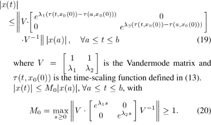
Theorem 2: Let and be two distinct negative constants. Consider the nonlinear system (15a)–(15c) in which the con-stants and are determined by (17). Suppose the sign of is constant for some time interval ( , ).

Then, every solution of (15a)–(15c) sat-isfies the following inequalities:

(19) where is the Vandermode matrix and

is the time-scaling function defined in (13).

, , with

(20)

Remark 3: Theorem 2 gives estimates for the effect of pole

placement. For example, the convergence rate can be computed using inequalities (14) and (19), and transient behavior (max-imum overshoot) can be estimated using inequality (20). Nu-merical methods can also be employed to minimize , thus improving transient behavior. Furthermore, observations con-cerning the robustness of the closed-loop system (15) can also be made, but since space is limited here and they do not affect our topic, we omit the details and refer readers to [18].

C. Fast Parking Control by Employing Tracking Controllers

In this subsection, we present a solution to the parking problem based on the tracking controller design given in preceding subsections; we assume Assumption (P) holds throughout this subsection. Given Proposition 1, we need only solve the TCP for the modified trajectory. Condition C2) from Theorem 1 remains to be verified. To this end, let

be the function in (6) for some positive constant , and be the period. Then, by the definition of , there exists a

such that . Since is continuous

and periodic, there exists a positive constant such that

, . Let .

By the periodic property of , for any , there exists a such that

, where is the constant given in (6). This implies

that ,

. Thus, the following inequality holds:

In particular, the Condition C2) holds for the modified desired angular velocity defined in (6) with . In view of Theorem 2, it is convenient to set , , when

applying the pole-placement method. Theorem 3 then follows from Proposition 1, Theorem 1 and (17).

Theorem 3: Let and be two distinct negative constants, and be any positive constants, and be a piecewise continuous and bounded nonnegative function with , . Suppose Assumption (P) holds. Replace the modified trajectory and with the functions and defined in (6), and the PTCP is then solvable by the following controllers:

if

if (21)

where for any given positive constant , is any constant satisfying

, and and are as described in (22), shown at the bottom of the page.

Remark 4: The function is a tuning function. In most applications, tracking signals satisfy either Condition C1) or As-sumption (P). Roughly speaking, this situation can be referred to as being in tracking mode when Condition C1) holds and being in parking mode when Assumption (P) holds. Given Theorem 1, it is preferable to set the tuning function to a nonzero value in tracking mode, but according to Theorem 2, it is preferable to set the tuning function equal to zero in parking mode in order to use the pole-placement method to improve parking performance. The controller proposed here solves the tracking and parking problems at the same time according to Theorem 1 and Theorem 3 by choosing suitable tuning functions and adding virtual tracking signals to the original tracking tra-jectory. Although a single controller was proposed in [11] and [21] to solve a similar problem, it was found that the conver-gence rate was very slow in parking mode. However, the con-troller proposed here can achieve exponential convergence on the parking problem via Theorem 1. This is demonstrated by means of an interesting experiment in the next section. It was also observed that the controllers presented in the papers men-tioned above cannot be extended to nonholonomic systems with orders higher than three due to their highly nonlinear structures. By contrast, the method proposed in this paper can be easily gen-eralized to higher dimension nonholonomic systems. In fact, a successful application of the idea presented in this paper to the parking control of an underactuated ship was recently given in [19].

IV. SIMULATIONS ANDEXPERIMENTALRESULTS

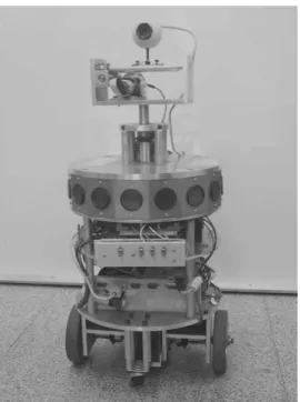
Fig. 1 shows the experimental mobile robot developed in the Intelligent System Control Integration Lab at National Chiao Tung University, Taiwan, R.O.C. It has two independent dc-servo-driven wheels and two casters for balance. Motion is controlled by adjusting the velocities of the left and right wheels via a two-axis motion control card based on a TMS320F240

Fig. 1. Experimental mobile robot developed in the Intelligent System Control Integration (ISCI) laboratory at National Chiao Tung University.

Fig. 2. Block diagram of the wheel motor control system; v = [v v ] is the velocity command vector, and v = [v w ] is the velocity vector of the robot.

DSP chip from Texas Instruments (TI). Fig. 2 depicts the block diagram of the wheel motor control system. In the figure, is the velocity command vector, where and denote the velocity commands to the left and right wheels, respectively. is the velocity vector of the robot, where and denote, respectively, the current linear and angular velocities of the robot. The onboard industrial PC only needs to send the velocity commands to the DSP chip, which manages the velocity servo control. Communication between the PC and the motion control card is through an RS-232 serial port.

The proposed parking controller was first verified by com-puter simulation and then verified by experiments with the mobile robot. The algorithm for estimating robot position is implemented on the PC, which samples the left and right wheel velocities to calculate the current pose of the robot. The velocity of each wheel , is measured based on the signals

from the shaft encoders mounted on the motors. The formula for this pose estimator is

(23)

(24) where is the distance between two drive wheels, and are, respectively, the current linear and angular velocities of the robot, and denotes the sampling period of the PC. In this case,

and .

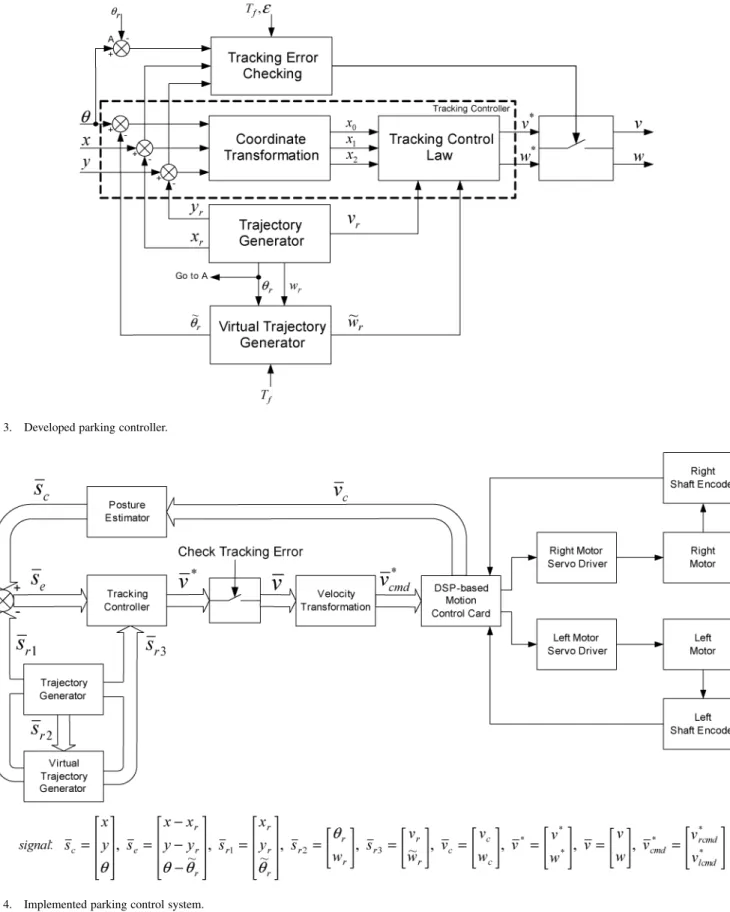
The architecture for realization of the proposed parking con-troller is presented in Fig. 3. The functions of the blocks shown in Fig. 3 are listed below:

1) coordinate transformation: transform coordinates using (3);

2) tracking control law: compute desired velocities using (22);

3) trajectory generator: generate desired tracking trajecto-ries, e.g., (26a)–(26e);

4) virtual trajectory generator: redesign trajectories using (6); and

5) tracking error checking: compute tracking errors

If and , stop executing the tracking control law; otherwise, keep tracking.

and are, respectively, the desired error bound and finish time for the desired trajectory tracking. They are given in the task specification. The desired velocities and , calculated by the tracking controller, are transformed into left- and right-wheel velocity commands using

(25) Fig. 4 shows the complete parking control system constructed using the proposed algorithm. The functions of the blocks shown in Fig. 4 are listed below:

1) DSP-based motion control card: estimate robot velocities using (23);

2) pose estimator: estimate robot positions using (24); and 3) velocity transformation: compute velocity commands

using (25).

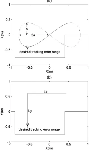
Two trajectories, parallel-parking and back-into-garage, were selected to verify the performance of the proposed parking con-troller. Fig. 5(a) illustrates the parking place and the parallel parking path, where and represent, respectively, the long and short axes. In the simulation and experiment, the constants

and were set to and . The

trajec-tory is given in (26a)–(26e). Fig. 5(b) shows the parking place and the back-into-garage path, where , are the horizontal and vertical distances between the initial and target positions, and , are the desired linear and angular velocities. In the experiment, these constants were set to m,

Fig. 3. Developed parking controller.

Fig. 4. Implemented parking control system.

m s and rad s. The trajectory equa-tions are given in (28a)–(28e).

In practical applications, a desired error bound must be specified. One way to determine this value is to consider tracking errors in individual axes. We set the desired tracking error to for each axis, thus is 0.1117

. As soon as the tracking error drops below (see Fig. 6) for some , the controller is set to zero and then the robot stops. The parameters ( , ) are used to match the attainable velocity of the mobile robot. In the experiment, was always equal to 1 and a small value was selected for . Experience gained in computer simulations

Fig. 5. Parking tasks and designed trajectories for the experiments.

suggested setting near 0.1. The nonnegative continuous function was designed according to Theorem 1 and Theorem 3. The parameters ( , ) were determined using Theorem 2, and a numerical method was applied to achieve acceptable transient behavior and convergence rate. Here, we selected various locally optimal parameters ( , ) for each experiment. It would be interesting to find globally optimal parameters for the parking controller and optimize performance with . This may be a direction for future study.

After resolving parameters, ( , ), we verified the tracking and docking performance of the parking controller using parallel-parking and back-into-garage trajectories. The parallel-parking experiment demonstrates the transient behavior and parking performance of the proposed parking controller, and the back-into-garage experiment verifies the ef-fect the nonnegative continuous function has on tracking performance.

A. Parallel-Parking Experiment

We utilized an 8-shaped trajectory [21] in this experiment. Let with . The model that generated the trajectories is delineated below.

• Parallel-parking path (see (26a)–(26e), shown at the bottom of the next page).

TABLE I

PARAMETERSUSED IN THEPARALLELPARKING

SIMULATION ANDEXPERIMENTS

Let . and can

then be found according to (6) as follows:

(27)

where parameter with

. Roughly speaking, given in the parallel-parking path satisfied Condition C2) for

, hence, according to Theorem 1, could be set to zero for the parallel parking experiment. The locally optimal parameters used in this experiment are shown in Table I.

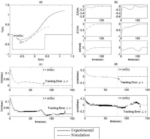
Fig. 6 presents the parallel-parking simulation and experi-mental results. The dotted lines represent computer simulation results, the solid lines the corresponding experimental ones. In Fig. 6(a), we see that the simulation trajectory converged rapidly to the desired path as expected. The tracking-error simulation results in Fig. 6(b) show that the proposed parking controller achieved locally exponential convergence.

Fig. 6(c) and (d) shows the recorded motion control card out-puts, i.e., the robot’s linear and angular velocities. The leaders in Fig. 6(c) and (d) indicates, respectively, the finish times of the desired tracking trajectory . As stated in Theorem 3, the parking controller is in the tracking mode when , and changes to parking mode when . When the con-troller is in parking mode and the tracking error drops below the desired error bound, it shuts down. Therefore, the simulation re-sults in Fig. 6 demonstrate that the proposed controller stayed in the tracking mode even when the tracking error was smaller than the desired error bound until , and

for all , meaning the conditions for stopping the con-troller were satisfied.

We observe that in Fig. 6(a), although the simulation trajectory rapidly converged to the desired trajectory, the experimental robot trajectory did not. This was caused by a shaft encoder truncation error and a quantization error from the velocity command, . Our robot’s dc motors are connected to the wheels via a 19:7:1 reduction gear and shaft encoders are mounted on the motor axes. Encoder resolution is 2000 pulses (counts) per revolution, which yields

pulses per wheel revolution. The wheel diameter in our design is 125 mm. Hence, the actual encoder resolution is

pulses/mm of wheel displacement. The servo control sampling time is 1 ms. Thus, the minimum observable velocity from the encoder output is 1000 pulses/s, which, given the encoder’s resolution, is equal to

mm/s or 0.01 m/s. In other words, because of encoder res-olution limitations and servo loop sampling time, estimation of each wheel’s velocity is truncated to 0.01 m/s. This is the source of the robot’s velocity measurement truncation error.

Fig. 6. Parallel parking simulation and experimental results. (a) Position variations. (b) Tracking errors. (c) Linear velocity of the center point,v . (d) Angular velocity,w .

The velocity commands and are quantized to 0.01 m/s in our design. Note that the quantization error in the velocity command is dependent on the bit resolution of the mo-tion control card, but the truncamo-tion error is not. We designed the quantization error to be equal to the truncation error. As the robot converges to the target position, the truncation and quan-tization errors cause large tracking errors because the velocity command is small around the goal [17]. In Fig. 6(c), the ex-perimental result shows that when the linear velocity was lower than 0.05 m/s, these errors greatly affected the practical linear

velocity. Hence, in practice, the robot cannot converge to the de-sired trajectory at any time before . In order to verify this, we included these errors in the computer simulation and the results are given in Fig. 7. In Fig. 7(a), we see that the practical results and the simulation ones, including truncation and quanti-zation errors, are quite consistent. Fig. 7(b) shows that the three tracking errors all converged to zero up to the given error bound as expected, even with the system’s error effects.

Fig. 7(c) and (d) shows the robot’s recorded linear and an-gular velocities. In the figure, the simulation results show that

(26a) (26b) (26c)

(26d)

Fig. 7. Experimental results with parallel parking truncation and quantization errors. (a) Position variations. (b) Tracking errors (c) Linear velocity of the center point,v . (d) Angular velocity, w .

the tracking error was larger than the desired error bound at time and that the controller kept tracking a virtual trajec-tory until the tracking error was below the desired error bound. Thus, the proposed parking controller overcame this problem al-though the situation was not considered in the design phase. This is because a virtual trajectory was redesigned for the controller when , and thus transformed the parking problem into a tracking problem. Hence the robot remained in tracking mode until its tracking errors converged to the desired error bound.

In order to emphasize the parking performance of the pro-posed parking controller, we compared it to the saturation feed-back controller proposed in [21]. The experimental results are given in Fig. 8. The dotted lines represent the results from the saturation feedback controller, the solid lines the corresponding results from the proposed parking controller. In Fig. 8(a), we see that the saturation feedback controller trajectory did not con-verge to the desired path. This shows that the saturation feed-back controller cannot solve the parking problem efficiently due to the slow convergence rate. A virtual trajectory was redesigned for the parking controller proposed here to solve the problem when , and the robot remains in tracking mode until its tracking errors converge to the desired error bound. There-fore, combining motion planning with tracking control enhances parking performance such that previous parking control limita-tions become more amenable to solution.

In Fig. 8(b), we see that when the proposed parking con-troller’s tracking errors all converge to zero, the robot has reached the target position, while the saturation feedback controller still shows tracking errors. Fig. 8(c) and (d) depicts the robots’ recorded linear and angular velocities. These simu-lation and experimental results demonstrate that the proposed parking controller not only solves the general parking problem, but also guarantees rapid convergence rates. This shows that in practice, the parking problem can be solved by combining motion planning with tracking control.

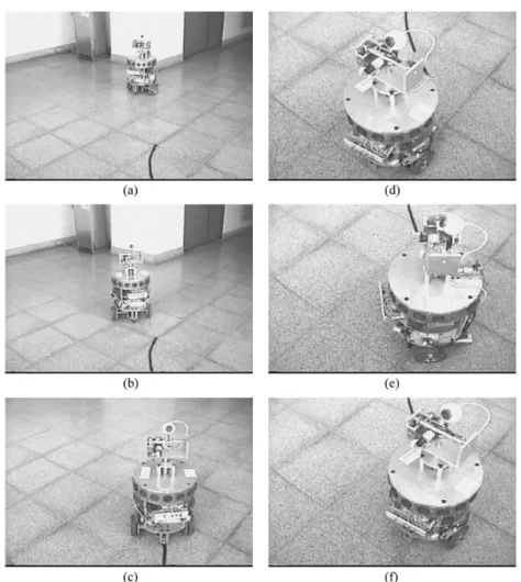
Fig. 9 shows photos of a robot motion sequence during the parallel parking experiment, the black line on the floor indicates the desired trajectory. In Fig. 9(a), the controller is turned on and the robot starts to track the desired trajectory. In Fig. 9(b) and (c), the robot tracks the desired trajectory as it moves to-ward the target position. In Fig. 9(d) (time ), the robot is near the target position, but the tracking error is still larger than the desired tracking error. In Fig. 9(e), the robot is tracking the de-sired virtual trajectory. In Fig. 9(f), the robot has arrived at the target position and the tracking error is smaller than the desired tracking error, so the parking procedure stops.

B. Back-Into-Garage Parking Experiment

This experiment verifies the effect of the nonnegative con-tinuous function on tracking performance. We utilized an

Fig. 8. Comparison of the proposed parking controller and the saturation feedback controller proposed in [21]. (a) Position variations. (b) Tracking errors. (c) Linear velocity of the center point,v . (d) Angular velocity w .

L-shaped trajectory in this experiment. Let

. The model that generated the tra-jectories is delineated below

(28a)

(28b)

(28c)

(28d)

(28e)

where ( , ), ( , ) denote, respectively, the robot’s ini-tial and terminative coordinates. In the simulation and

experi-ment, they were set at m m ,

m m .

TABLE II

PARAMETERSUSED IN THEBACK-INTO-GARAGESIMULATION ANDEXPERIMENTS

Let, , and can

then be found according to (6)

(29) where parameter . Locally optimal parameters used in the experiment are given in Table II.

From Remark 4 after Theorem 3: is a tuning function that smoothly transforms tracking situations into parking situ-ations. Since the back-into-garage path only roughly satisfies Condition C1) for all , as suggested by Remark 4, should be set to a positive value before , and then changed to a zero function to perform pole placement according to Theorem 2. Details of the selection for this experiment are as follows:

.

(30) Fig. 10(a)–(e) depicts results from the back-into-garage parking experiment. In the figure, the solid lines represent experimental

Fig. 9. Sequence of motions during the parallel parking experiment.

results using (30). For comparison, we carried out the same parking experiment with as a zero function, such that

(31) The experimental results of using (31) are shown as dotted lines in Fig. 10(a)–(e). We can see that the tracking performance and convergence rate behaved satisfactorily when was a positive continuous function, before s. The effect of the tuning function is therefore verified by these experimental results.

V. CONCLUSION

A novel fast parking controller for nonholonomic mobile robots based on a motion planning approach and tracking control design has been proposed and demonstrated. It solves parking problems by adding a redesigned virtual trajectory to the original trajectory. Practical experimental results verified its satisfactory convergence results. In contrast to results presented in [21], the motion planning method proposed in this paper can be extended to other higher order nonholonomic systems. An interesting application to underactuated ships can be found in [19]. Future work may focus on improving parking performance, such as in the area of robustness as it relates to uncertainty in the model and other disturbances.

APPENDIX

PROOF OFTHEOREM1

A stability criterion is recalled first. Its proof can be found in [20]. Throughout this appendix, it is said that a statement holds almost everywhere (a.e.) if the Lebesgue measure of the set is false is zero [31].

Proposition A1: Consider the following system

(A1) where is continuous in , uniformly in , and uniformly bounded on , for each , where is an open ball centered at the origin with radius . Let

be a continuously differentiable, positive–definite and proper function such that

(A2) for all , all where the function is contin-uous in , uniformly in , and uniformly bounded on , for each . The origin is then uniformly globally

asymptot-ically stable provided that the following condition holds.

A1) For every time sequence , with , and every bounded continuous function that satisfies

Fig. 10. Comparison of tracking performance using two differentk (t) values. (a) Position variations. (b) Tracking errors. (c) Linear velocity of the center point v . (d) Angular velocity w . (e) A “zoom-in” graph of position variations.

, a. e., and the following integral equation:

(A3)

we have .

With the controller (9), the closed-loop system of the tracking error model (4a)–(4c) can be written into the following equa-tions:

(A4) (A5) (A6)

where . The closed-loop

system (A4)–(A6) is in the form of (A1). Since all the time func-tions appeared in the differential equafunc-tions are bounded, it is easy to see that the function is continuous in , uniformly in , and uniformly bounded on , for each . It is also seen that the Lyapunov function defined in (8) is a continuously differentiable, positive–definite and proper func-tion that satisfies the inequality (A2) with

(A7) through (10). Moreover, the function is also continuous in , uniformly in , and uniformly bounded on , for each . It remains to check the condition (A1) holds to guar-antee the uniformly globally asymptotical stability of the origin

in view of Proposition A1. To this end, we need the following lemma.

Lemma A1: Let and be two sequences of

real-valued functions defined on with and , for all , all in , and some positive constants and . Suppose the following conditions hold:

(A8)

for some (A9)

Let be a continuous function defined on that satisfies (A10) for some constant . Assume that the following equation

a.e. (A11)

holds. We have then and .

Proof: Notice that (A8) implies that

(A12) Let us first show that implies . Indeed, by (A10), is a constant function when . If is not a zero function, then we have , a.e., in view of (A11). Consequently, by (A12) and Lebesgue dominate theorem [31]

Thus, we reach a contradiction according to the inequality (A9). In the following, we show that and complete the proof of the lemma. We will prove it by contradiction. Suppose .

From (A10), the limit can

be defined, . It results in

(A13)

We claim that there exists a such that . If the claim is false, we have , . Then, there exists a measure zero set such that

, through (A11). According to (A12), this implies that

We reach a contradiction in view of (A13). Thus, the claim is true. Particularly, we can define

and . By the

defini-tions, it can be seen that , .

Again from (A11), there exists a measure zero set such that

, By (A12)

and Lebesgue dominate theorem, this implies that the following expressions hold:

and

Thus, in view of (A13)

(A14) Since is a continuous function, it can be seen that

by the definitions. Consequently, we have , and hence, in view of (A14). We reach another contradiction. It completes the proof.

Now, let us check condition (A1) by employing Lemma A1. Let be any time sequence with and ( , , ) be any bounded continuous functions such that

, a. e., and the following equations hold: (A15) (A16) (A17) where

Notice that the equation

, a. e., is equivalently to saying that

a.e. (A18)

a.e. (A19) and

a.e. (A20)

Since is a continuous function, (A18) implies that is a zero function [31]. Thus, (A15) is reduced to the (A8), i.e., the condition (i) in Lemma A1 holds. Moreover, (A16) is also reduced to

by using Lebesgue dominate theorem [31] and (A19). In par-ticular, is a constant function. Let ,

and , , . (A19)

is then equivalent to (A11) and (A17) is reduced to (A10) by using the (A8), (A19), and (A20). Now, let us verify condition ii) in Lemma A1 by assuming the Condition C2). If Condition C2) holds, there exist three positive constants , and so that (A21)

for some sequence with . Since is

contained in the compact set , there exists a subsequence of converging to a point . This results in

Thus, ii) in Lemma A1 holds under Condition C2). It can be

concluded that , and in view

of Lemma A1. Thus, condition (A1) holds and the origin of the closed-loop system is uniformly globally asymptotically stable by using Proposition A1 and Condition C2). On the other hand, assume that , . Equation (A20) implies that , a.e. Since is a continuous function, this implies that is a zero function. Notice that the (A15) is reduced to

(A22)

due to the fact that is a zero function, is a constant function and . Using a similar argument as in the pre-vious discussion, condition (C1) implies that there exist four positive constants , , , so that

If , , , by (A22).

This implies that (ii) in Lemma A1 holds and again

by Lemma A1. We reach a contradiction. Thus, and

we conclude that , , and under

Condition C1) and the assumption , .

Again, condition (A1) holds and the origin of the closed-loop system is uniformly globally asymptotically stable via Propo-sition A1. A similar argument can be applied to the linearized closed-loop system, that can also be described by (A4)–(A6) with and . Consequently, it can be concluded that the origin of the linearized system is also uniformly glob-ally asymptoticglob-ally stable. Hence, the origin of the closed-loop system is locally exponentially stable [16]. This completes the proof.

ACKNOWLEDGMENT

The authors would like to thank C.-C. Chien and K.-M. Yan of the Intelligent System Control Integration Lab, National Chiao Tung University, for their assistance in construction of the mo-bile robot. The authors would also like to thank the Associate Editor, Prof. K. L. Moore, and the anonymous referees for their constructive comments and suggestions.

REFERENCES

[1] A. Astolfi and W. Schaufelberger, “State and output feedback stabiliza-tion of multiple chained systems with discontinuous control,” in Proc.

IEEE 35th Conf. Decision Control, Japan, 1996, pp. 1443–1448.

[2] A. M. Bloch, M. Reyhanoglu, and N. H. McClamroch, “Control and sta-bilizability of nonholonomic dynamic systems,” IEEE Trans. Automat.

Contr., vol. 37, pp. 1746–1757, Nov. 1992.

[3] R. W. Brockett, “Asymptotic stability and feedback stabilization,” in

Differential Geometric Control Theory, R. W. Brockett, R. S. Millman,

and H. H. Sussmann, Eds. Cambridge, MA: Birkhauser, 1983, pp. 181–191.

[4] C. C. de Wit, H. Berghuis, and H. Nijmeijer, “Practical stabilization of nonlinear systems in chained form,” in Proc. IEEE 33th Conf. Decision

Contol, Lake Buena Vista, FL, 1994, pp. 3475–3480.

[5] C. de Wit Canudas, B. Siciliano, and G. Bastin, Eds., Theory of Robot

Control. London, U.K.: Springer-Verlag, 1996.

[6] C. C. de Wit and O. J. Sordalen, “Exponential stabilization of mobile robots with nonholonomic constraints,” IEEE Trans. Automat. Contr., vol. 37, pp. 1791–1797, Nov. 1992.

[7] C. C. Chang and K. T. Song, “Environment prediction for a mobile robot in a dynamic environment,” IEEE Trans. Robot. Automat., vol. 13, pp. 862–872, Dec. 1997.

[8] C. T. Chen, Introduction to Linear System Theory. New York: Holt, Rinehart and Winston, 1986.

[9] J. M. Coron, “Global asymptotic stabilization for controllable systems without drift,” Math. Contr., Signals, Syst., vol. 5, pp. 295–312, 1992. [10] W. E. Dixon, D. M. Dawson, E. Zergeroglu, and F. Zhang, “Robust

tracking and regulation control for mobile robots,” Int. J. Robust

Non-linear Contr., vol. 10, pp. 199–216, 2000.

[11] K. D. Do, Z. P. Jiang, and J. Pan, “A universal saturation controller de-sign for mobile robots,” in Proc. IEEE 41st Conf. Decision Control, Las Vegas, NV, 2002, pp. 2044–2049.

[12] , “Universal controllers for stabilization and tracking of underactu-ated ships,” Syst. Contr. Lett., vol. 47, pp. 299–317, 2002.

[13] J. P. Hespanha, D. Liberzon, and A. S. Morse, “Logic-based switching control of a nonholonomic system with parametric modeling uncer-tainty,” Syst. Contr. Lett., vol. 38, pp. 167–177, 1999.

[14] Z. P. Jiang, “Robust exponential regulation of nonholonomic systems with uncertainties,” Automatica, vol. 36, pp. 189–209, 2000.

[15] Z. P. Jiang and H. Nijmeijer, “Tracking control of mobile robots: a case study in backstepping,” Automatica, vol. 33, pp. 1393–1399, 1997. [16] H. K. Khalil, Nonlinear Systems. New York: Macmillian, 1992. [17] B. M. Kim and P. Tsiotras, “Controllers for unicycle-type wheeled

robots: theoretical results and experimental validation,” IEEE Trans.

Robot. Automat., vol. 18, pp. 294–307, 2002.

[18] T. C. Lee, “Practical stabilization for nonholonomic chained systems with fast convergence, pole-placement and robustness,” in Proc.

IEEE Int. Conf. Robotics and Automation, Washington DC, 2002, pp.

3534–3539.

[19] T. C. Lee, Tracking of Underactuated Ships via a Relaxed PE Condition, to be published.

[20] T. C. Lee and B. S. Chen, “A general stability criterion for time-varying systems using a modified detectability condition,” IEEE Trans. Automat.

Contr., vol. 47, pp. 797–802, May 2002.

[21] T. C. Lee, K. T. Song, C. H. Lee, and C. C. Teng, “Tracking control of unicycle-modeled mobile robots using a saturation feedback controller,”

IEEE Trans. Contr. Syst. Technol., vol. 9, pp. 305–318, Mar. 2001.

[22] D. A. Lizarraga, P. Morin, and C. Samson, “Non-robustness of contin-uous homogeneous stabilizers for affine control systems,” in Proc. IEEE

38th Conf. Decision Control, Phoenix, AZ, 1999, pp. 855–860.

[23] R. T. M’Closkey and R. M. Murray, “Exponential stabilization of drift-less control systems using homogeneous feedback,” IEEE Trans.

Au-tomat. Contr., vol. 42, pp. 614–628, May 1997.

[24] P. Morin and C. Samson, “Control of nonlinear chained systems: from Routh-Hurwitz stability criterion to time-varying exponential stabilizers,” IEEE Trans. Automat. Contr., vol. 45, pp. 141–146, Jan. 2000.

[25] , “Robust stabilization of driftless systems with hybrid open-loop/feedback control,” in Proc. ACC, Chicago, IL, 2000, pp. 3929–3933.

[26] , “Practical stabilization of driftless systems on Lie groups,” in

Proc IEEE 41st Conf. Decision Control, Las Vegas, Nevada, 2002, pp.

4272–4277.

[27] R. M. Murray and S. S. Sastry, “Nonholonomic motion planning: steering using sinusoids,” IEEE Trans. Automat. Contr., vol. 38, pp. 700–716, May 1993.

[28] K. S. Narendra and A. M. Annaswamy, Stable Adaptive

Sys-tems. Englewood Cliffs, NJ: Prentice-Hall, 1989.

[29] I. E. Paromtchik and C. Laugier, “Autonomous parallel parking of a non-holonomic vehicle,” in Proc. IEEE Intelligent Vehicles Symp., Tokyo, Japan, 1996, pp. 13–18.

[30] J. B. Pomet, “Explicit design of time-varying stabilizing control laws for a class of controllable systems without drift,” Syst. Control Lett., vol. 18, pp. 467–473, 1992.

[31] W. Rudin, Real and Complex Analysis. New York: McGraw-Hill, 1987.

[32] C. Samson, “Control of chained systems application to path following and time-varying point-stabilization of mobile robots,” IEEE Trans.

Au-tomat. Contr., vol. 40, pp. 64–77, Jan. 1995.

[33] C. Samson and K. Ait-Abderrahim, “Feedback control of a nonholo-nomic wheeled cart in Cartesian space,” in Proc. IEEE Int. Conf.

Robotics and Automation, Sacramento, CA, 1991, pp. 1136–1141.

[34] K. T. Song and C. E. Li, “Tracking control of a fee ranging automatic guided vehicle,” Control Eng. Practice, vol. 1, no. 1, pp. 163–169, 1993. [35] K. T. Song and L. H. Sheen, “Heuristic fuzzy-neuro network and its application to reactive navigation of a mobile robot,” Fuzzy Sets Syst., vol. 110, no. 3, pp. 331–340, 2000.

[36] O. J. Sordalen and O. Egeland, “Exponential stabilization of nonholo-nomic chained systems,” IEEE Trans. Automat. Contr., vol. 40, pp. 35–49, Jan. 1995.

[37] M. Vidyasagar, Nonlinear Systems Analysis. Englewood Cliffs, NJ: Prentice-Hall, 1993.

Ti-Chung Lee was born in Taiwan, R.O.C., in 1966. He received the M.S. degree in mathematics and the Ph.D. degree in electrical engineering from the National Tsing Hua University, Hsinchu, Taiwan, in 1990 and 1995, respectively.

He is currently an Associate Professor in the Department of Electrical Engineering, Ming Hsin University of Science and Technology, Hsinchu. His main research interests are nonlinear control systems, nonholonomic systems, and robot control.

Chi-Yi Tsai was born in Kaohsiung, Taiwan, R.O.C., in 1978. He received the B.S. and M.S. degrees in electrical engineering from National Yunlin Technology University, Yunlin, Taiwan, in 2000 and 2002, respectively. He is currently working toward the Ph.D. degree in electrical and control engineering at the National Chiao Tung University, Hsinchu, Taiwan.

His research interests include visual motion plan-ning of mobile robots, visual servoing, and computer vision.

Kai-Tai Song (A’91) was born in Taipei, Taiwan, R.O.C., in 1957. He received the B.S. degree in power mechanical engineering from National Tsing Hua University, Hsinchu, Taiwan, in 1979, and the Ph.D. degree in mechanical engineering from the Katholieke Universiteit Leuven, Belgium, in 1989.

He was with the Chung Shan Institute of Science and Technology from 1981 to 1984. Since 1989, he has been on the faculty and is currently a Professor in the Department of Electrical and Control Engi-neering, National Chiao Tung University, Hsinchu, Taiwan. His areas of research interest include mobile robots, image processing, visual tracking, sensing and perception, embedded systems, intelligent system control integration, and mechatronics.