Prandtl-Reuss Elastoplasticity: On-Off Switch and Superposition Formulae

Please cite this paper as follows:

Hong-Ki Hong and Chein-Shan Liu, Prandtl-Reuss Elastoplasticity: On-Off Switch

and Superposition Formulae, International Journal of Solids and Structures, Vol.34,

0 1997 Elwier Science Ltd PII : SOO20-7683(W)OOO2fi-7

AU rights reserv&. Printed in Great Britain 002&7683/97 $17.00 + .OO

PRANDTL-REUSS

ELASTOPLASTICITY

: ON-OFF

SWITCH AND SUPERPOSITION

FORMULAE

H.-K. HONG and C.-S. LIU

Department of Civil Engineering, Taiwan University, Taipei, Taiwan (Received 12 July 1996 ; in revised form 3 January 1997)

Alas&act-Constitutive postulates for Prandtl-Reuss elastoplasticity are selected. Based on them, sufficient and necessary conditions for plastic irreversibility are found to be the yield condition and the straining condition. This is then analyzed and it is pointed out that Prandtl-Reuss elastoplasticity is nothing but a two-phase linear system with an on-off switch, which is operated in the pace of an intrinsic measure of plastic irreversibility. Then the temporally global concept of the switch-on time I, and the switch-off time r,and their determination and bound estimation is developed. Owing to the implicit linearity, superposition formulae for the stress response are discovered. As an example, the exact constitutive solutions for circular paths based on the superposition formulae are obtained and 1, and to,rare determined. 0 1997 Elsevier Science Ltd.

1. AXIOMS AND INTRODUCTION

In this paper we un&ze the Prandtl-Reuss model and attempt to achieve a deeper under- standing of its underlying structure ; more precisely speaking, we explore the switching of the mechanism of plastic irreversibility and the implicit principle of superposition of responses. Although our consideration is limited to the Prandtl-Reuss model, the former issue is considered as typical in the models of plasticity, whereas the latter may exist in some classes of plasticity models more complicated than it.

The elastoplasticity of solid materials proposed by Prandtl (1924) and Reuss (1930) is re-postulated as in the following system of axioms :

e =

Y+P,

₍₁₎

S = 2GC’, (2)

l’s =

2hP, ₍₃₎

a..=

li,

where (7)

withy= 1 being the yield condition. The two material constants, namely the shear modulus G and the shear yield strength h, are both positive. The bold-faced e, ee, &’ and s are, respectively, the deviator% tensors of strain, elastic strain, plastic strain, and stress, all symmetric and traceless, whereas 1 is a scalar. All the e, ee, 8, s and 1 are functions of one and the same independent variable, which in most cases is taken either as the usual time or as the arc length of the controlled strain path ; however, for convenience, the independent

4282 H.-K. Hong and C.-S. Liu

S12 A

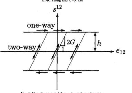
Fig. 1. One-dimensional shear stress-strain diagram.

Fig. 2. Allowable stress regionf6 l-a compact spherical geometry.

variable no matter what it is will be simply called “time” and given the symbol t. A superimposed dot denotes a differentiation with respect to time, d/dt. Without loss of generality, it is also postulated that with the above differential model there is a time instant designated as t = to, called the zero-value (or annealed) time, before and at which the material is in the zero-value (or annealed) state in the sense that the relevant values e(t,,), e’(t,,), @(to), s(t,,) and A(&) are all zero.

The Prandtl-Reuss model is well known as the simplest yet most useful three-dimen- sional constitutive law for describing a class of mechanical behaviors of linearly elastic- perfect plasticity, of which a typical one-dimensional stress-strain diagram is shown in Fig. 1. The essential feature of this diagram is the flat yield which produces a sharp stress boundary between elastic behavior at infinitely many parallel two-way line segments and unrestricted plastic flow at two heavy horizontal one-way lines.

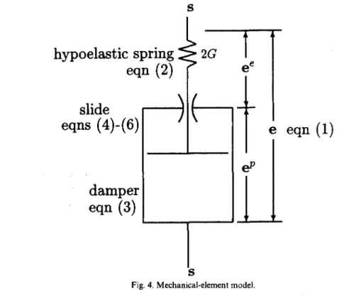
A mechanical-element model and two diagrams displayed in Figs 2-4 may help explain the meaning of axioms (l)-(6), hopefully without misleading.? To illustrate the inequality (4), Fig. 2 displays schematically the set of allowable stress states as a closed ball in the s stress space, which consists of an open ball of elastic states and its boundary, a hypersphere with plastic irreversibility. The effect of the complementary trios (4)-(6) may be summarized in the heavy two-segment line in Fig. 3, which hints that there exist just two phases of allowable states, the on and offphases of the plastic mechanism, corresponding to the two segments. This topic is very important, but was conventionally addressed in the language of loading, neutral loading and unloading criteria, and will be explored in Section 3. It appears from Fig. 4 that the Prandtl-Reuss model might be something like the Maxwell model of viscoelasticity ; however, the damper in Fig. 4 is, in addition to the piston-cylinder construction for simulating eqn (a), also equipped with an on+@ switch, which is sketched in Fig. 4 as a (Saint Venant) friction-slide for simulating eqns (4)-(6). Moreover, everrthe

Fig. 3. The complementary trios (4)-(6) appear as (a) a two-segment lile composed of (b) two segments:Otheonphase{IzOandf=l)and~theoffp~ase{l=Oandf61}.

s

hypoelastic

spring

2G eqn (2) t

I

71

ee i e

ep

ll

slide

eqns (q-(6)

damper

ew

(3)

/ S

eqn

(1)

Fig. 4. Mechanical-element model.

piston-cylinder construction herein is not a usual one, as it is governed by the A-rate damper law

s-&f-

_.

I

in case dl > 0, instead of governed by the t-rate damper law

s=2h$.

(8)

(9)

As a consequence, the material in case d2 > 0 obeys the I-rate law of Prandtl-Reuss elastoplasticity

4284 H.-K. Hong and C.-S. Liu

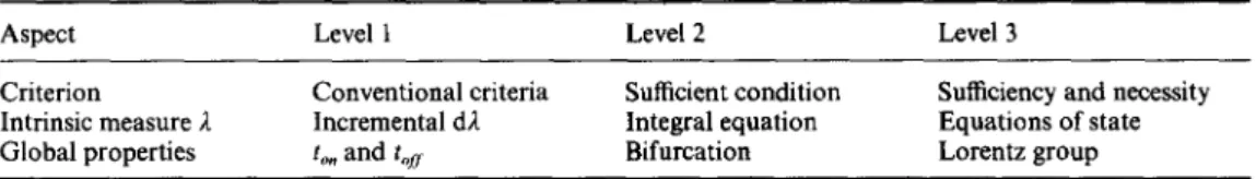
Table 1. Underlying structure of the plastic on-off switch

Aspect Level 1

Criterion Conventional criteria

Intrinsic measure I Incremental di Global properties r,, and tQti

Level 2

Sufficient condition Integral equation Bifurcation

Level 3

Sufficiency and necessity Equations of state Lorentz group

ids 1

zcdn+zhs=$

(10)

in the compact spherical geometry rather than the t-rate law of Maxwell’s viscoelasticity ids 1

zcdt+2hs=$

in the unbounded Euclidean geometry. The two geometries, as well as the two equations themselves, indicate that the time variations in the components in eqn (11) are uncoupled but those in eqn (10) are coupled through 1. One of the consequences of this is demonstrated in an interesting example in which the relaxation tests? of the two models are seen to be almost identical except that the Prandtl-Reuss model requires i > 0, for which the sufficient and necessary conditions are therefore very important and will be derived in Section 3. x involves t and 1; while t is the independent variable, a measure representing the world outside the material system ; 1 is a dependent variable, an intrinsic measure of the material system itself, measuring the degree of plastic irreversibility. The intrinsic measure A is indeed associated with the on-offswitch of the mechanism of plastic irreversibility. They lie in the core of the structure of plasticity and will be studied in Sections 3 and 4, and further in Sections 6 and 7.

To have a fuller and deeper understanding of the issue of the plastic on-off switch, it is supposed that the three aspects as listed in Table 1 should be explored and for each aspect the exploration could be advanced three levels deeper as suggested in the same table. As regards the aspect of the criterion of plastic irreversibility, the level 2 has recognized demarcation of only two cases, the plastic mechanism either switched-on or switched-off, rather than three or four cases often present in conventional criteria. Moreover, the criterion and the demarcation are indiscriminately applicable to hardening, softening and perfect plasticity [Hill (1958, 1967), Hong and Liu (1993), Liu (1993), Hashiguchi (1994)]. These were treated at level 2 in a statement of sufficiency; both sufficiency and necessity have been proved at level 3 [Hong and Liu (1993) Liu (1993)]. Regarding the aspect of the intrinsic measure of plastic irreversibility, ,I, its introduction into plasticity has lead to time- independent flow theories flourishing and some unconventional theories. Further at the level 2, an integral equation governing the evolution of 1 or its homeomorphism has been obtained, and the current state of response is completely determined once the history of 1 up to the current time is determined by solving the integral equation [Hong and Liou (1993)]. Instead of the history of I which contains an infinite number of real numbers, at level 3 only a finite number of the current values of an appropriate homeomorphism of 1 and its first few order time derivatives are needed in an equation-of-state representation for the current state of response. With regard to the aspect of global properties, such temporally global concepts as the switch-on time and the switch-off time are treated at level 1. Level 2 goes further to bifurcation analysis, i.e., analysis of qualitative change of material behaviors as material parameters and control parameters vary. At level 3 the nature of plasticity models is studied in the context of the Minkowski spacetime and Lorentz group. The present paper is confined to level 1 for the aspect of global properties and to level 2 for the aspect of the intrinsic measure, while the aspect of the criterion is studied down to level 3 ; of course, all the three aspects have been confined herein to the simplest, the Prandtl-Reuss model.

Recall that for linear elasticity and viscoelasticity the superposition principle allows us to present the general solution in terms of a finite number of particular solutions. Similarly, for a linear ordinary differential equation, or a system of such equations, a superposition principle is available in general. Around 1893, Sophus Lie and several other mathematicians posed the question whether superposition is restricted to linear equations or whether it can be generalized. Since then the methods of Lie groups and Lie algebras have been developed to identify and construct nonlinear differential systems for which superposition applies and to derive explicit superposition formulae [Anderson et al. (1982) ; Winter&z (1982)].

In a similar spirit, although plasticity models appear to be highly nonlinear, the Prandtl-Reuss model will be transformed in Section 5 into a two-phase linear system with an on-off switch. It will then be made clear that it is a system of linear algebraic equations during the off phase, but turns out to be a system of linear differential equations with variable coefficients in the on phase. Owing to the implicit linearity, superposition formulae for the stress response can be extracted, as to be derived in Section 8 and illustrated in more details in Section 9.3. The concept and results are introduced in plasticity for the first time, but the mathematics involved is much simplified for readability. Three consecutive block diagrams? in Section 5 provide a plain explanation how the superposition principle is discovered from a nonlinear Prandtl-Reuss equation to a feedback system and then to a linear augmented state equation.

The volumetric part of the Prandtl-Reuss behavior is linearly elastic and is thus excluded from the present study in order to focus on the more interesting elastic-plastic behaviors of the deviatoric part.

2. STRESS OPERATOR

Noting the positivity of G and h, we substitute eqns (2) and (3) into eqn (I), getting

which becomes upon defining 1 1. --6+2j+s=c, 2G -$( Ys) = 2G Ye, Y:=exp :J . ( ) The solution is

(12)

(13) (14)

which defines an operator that maps strain histories (or paths) into stress histories (or paths). Here t is the current time and ti is an initial time, at which initial conditions are prescribed. We note that the initial time tj is not necessarily the zero-value time to and the initial stress S(ti) does not necessarily vanish, for the material may suffer various loadings during manufacture and handling before it comes into use or reuse ; indeed, tj 2 to, s(ti) # 0 and Y(ti) # Y(t,,) = 1 in general. Obviously, the expression of eqn (15) that stress is in terms of the strain history is usable only if the Y history is already known. Thus, Y deserves more study, as will be pursued in the following two sections.

4286 H.-K. Hong and C.-S. Liu

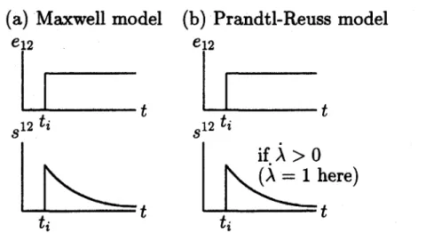
(a) Maxwell model (b) Prandtl-Reuss model

el2 el2

/+

kt

Fig. 5. Relaxation tests for (a) Maxwell’s viscoelastic model and (b) the Prandtl-Reuss elastoplastic model.

3. SWITCH OF PLASTIC IRREVERSIBILITY

In this section we shall see that the complementary trios (4) (5) and (6) enable the model to possess an on-off switch of the plastic mechanism, the switching criterion of which are derived right below. The inner product of s and eqn (12) is

1 fl.

-s*s+ ,,s*s = sac,

2G

(16)

where the dot between two tensors denotes the inner product ; e.g., s-C = S”kik If the yield conditionf= 1 is satisfied, the above equation becomes

h3;=s*i! iff= 1; ₍₁₇₎

recalling the positivity of h, we have

iff= 1, then s-6 > 0-n > 0; ₍₁₈₎

hence

v=l and s*r!>O}*ii>O. ₍₁₉₎

At this moment let us turn to Fig. 5. The conditions under which the Prandtl-Reuss materials exhibit the pseudo-relaxation curve? in Fig. 5(b) are both f = 1 and s se > 0, since they guarantee j > 0 according to the above statement (19). These can be done by, for example, for all t > ti

e, 2 (t) = constant,

so that

s”(t) =

J

h*(S’*(ti))* expT(ti- t),

P(t) = ?3(t) = 33(t) = 0,

₍₂₀₎

4287 d2(t) =

s’2(fi)exp;(t,-r),

h P,, (1) = - 2s’ ’ (t) ’ k**(f) = &*3(t) = l+,,(t) = 0, f(t) = 1, /i(t) = 1, as shown in Fig. 5(b).

On the other hand, if i > 0, eqn (6) assuresf = 1, which together with eqn (18) asserts that

i>O*u=l and s*c!>O}. (21)

Hence, from eqns (19) and (21), we conclude that the yield conditionf = 1 and the straining condition s * C > 0 are sufficient and necessary for plastic irreversibility i > 0. Considering this and the inequality (5) we thus reveal the following criteria for plastic irreversibility :

i >O ifff= 1 and s*e>O,

= 0 otherwise,

(22)

or via eqn (14)

I’

>O ifff=l and s*e>O,

= 0 otherwise. (23)

The “iff” and “otherwise” in the above mean “if and only if” and “ifff < 1 or/and s * e i 0,” respectively. According to the complementary trios (4)-(6), there are just two phases : 0 j > 0 andf= 1, and @ x = 0 and f 4 1. The complementary trios can be represented as the heavy two-segment line of Fig. 3(a), and in Fig. 3(b). the two phases are further distinguished as two segments. From the criterion (22) it is clear that @I corresponds to the on phase while @ to the off phase: In the on phase, A > 0, P > 0, the mechanism of plastic irreversibility is working, and the material exhibits elastoplastic behavior, while in the off phase, x = 0, P = 0, and_ the material is reversible and elastic. Thus eqn (22) (or eqn (23)) is called the on-off switching criterion for the on-off switch of the mechanism of plasticity.

The complementary trios (4)-(6) together with the expression (18) assert that

no matter whether in the on or off phases. Substituting eqns (2) and (3) into the above equation and considering the positivity of the two material constants, we obtain

Y.&f

=o.

₍₂₄₎

4288 H.-K. Hong and C.-S. Liu

*e

e

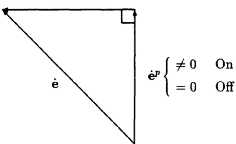
Fig. 6. Orthogonal decomposition of strain rate.

series as schematically depicted in Fig. 4 be an orthogonal vector addition as shown in Fig.

6. Hence we deduce that

lIelIZ = lFf7l’+ 11~112~ (25)

where llC]l := & is the Euclidean norm of & and so on. Furthermore, we can summarize Fig. 6, eqns (2) and (3) and the on-off switching criterion (22) altogether in one constitutive diagram for the Prandtl-Reuss model as in Fig. 7.

In passing it is worth noting that

&*V=V.i?pPQ ₍₂₆₎

by eqns (24) and (1). Materials which satisfy such an inequality e - &’ 2 0 are said to be kinematically stable [e.g., Lubliner (1984)].

i = 2Gk” S Switch-off _ If llsll = ah and SW 6~ > 0 Switch-on 6 Fig. 7.

lonl

(4

Constitutive diagram (0 perpendicular, II

cl

Off

(b)

4. MEASURE OF PLASTIC IRREVERSIBILITY

4289

It is noted that the flow model represented by the axioms (l)-(6) is a time-independent material model, because once dt is factored out, the differential eqns (l)-(3) and (5)-(6) become incremental equations independent of time. Equation (5) indicates that 1 is a time- like parameter and in the time-independent model plays the role of the arrow of time. The same can be said of Y because of eqn (14). In fact, either one, as evidenced in criteria (22) or (23) can serve as an intrinsic measure of plastic irreversibility, the calculation of which is crucially indispensable to the evaluation of the evolution of the material behavior, as has been partially reflected in eqn (15), and is the topic of investigation right below.

If the yield conditionf = 1 is satisfied, it follows from eqns (14) and (17) that

I’=;Ys.b,

which together with eqn (15) gives

m =

s

Y(ti)S(ti)*b(t)+ % I ‘e(t)*b(<)Y(<)dt. ‘i (27)

(28)

integrating and changing the order of integrations, we have

Y(t) = 1 +

s

[e(t) -e(ti)] *S(ri)

1 ’ h2 i.

Y(t.) +

2G2

’

[e(r) -e(t)] *e(t) Y(t) d{. (29) The above equation is a linear Volterra integral equation of Y. The existence and uniqueness of the solution Y(r) are guaranteed under essentially unrestricted condition on the e strain history.

We have noted that 1 and Y are intimately related by the definition (14). In fact, besides 1 and Y, there are other quantities, e.g., the Odqvist’s equivalent plastic strain k, dissipation A (herein defined as the dissipated energy per unit volume), etc., which are all intimately related in the sense that their differentials are the same up to a multiplicative constant (e.g., I = JGp = Jzlle”ll), or there exists a homeomorphism between any pair of them and the homeomorphism is a strictly increasing material function (e.g., for the Prandtl-Reuss model, li = hX and eqn (14) also). Therefore, any one of them can be chosen to play the pivotal role in the on-off switching criterion like (22), the role of an indicator of irreversible change of material, the role of so-called material age, intrinsic time, internal time, the arrow of time, etc., in this time-independent model.

In the rest of this section, we shall give an estimate of bounds on Y and I’ in order to probe the tendency of the evolution of this key measure. From eqns (3), (5) (6), (7) and (25~

n’ = Jzll~ll G Jwl,

which together with eqn (14) sets up the following bounds : Y(ti) < Y(f) < /A(tj, t) Y(ti) if ti < t, where

(30)

(31)

4290 H.-K. Hong and C.-S. Liu

(,/?G/h)IjBJ( is the largest eigenvalue of the state matrix A of the linear system (41) of the

on phase to be introduced in Section 5. Let

Thus, in the interval [te tb), the kernel b(t) -C(t) of the integral equation (28) is positive, and upon noting p(ti, 5) < p(ti, tb) the bounds of Yin this interval can be estimated by eqn (30) as follows :

Y(fO < Y(t) G /J(tiy fb) Y(ti) V< E(ti, tb)

Then we have an estimate of lower and upper bounds on Y:

Y, < I’< Y”,

where

(34)

,1

P,(t) = Y(Ci)E

_h2

l

[

jij S(h) * C(t) + e(t) s MO - e(G)1

J

,

(35)

(33)

* HO + b(t) ’ [e(t) -

e(tdlP.(ti,

tb) 3

. (36)

5. TWO-PHASE LINEAR SYSTEM

If the mechanism of plasticity is switched off, the Prandtl-Reuss model (l)-(6) reduces to

% = 2GB, ₍₃₇₎

which is linear and instantaneous. Integrating both the sides of the above equation from the initial time ti to the current time t yields 3.

s(t) = s(tJ+-2G[e(t)-e(ti)]. (38)

On the other hand, if the mechanism of plasticity is switched on, the Prandtl-Reuss model, like other plasticity models, appears to be nonlinear as manifested in the following nonlinear equation

Sf -s Gs*b = 2Ge,

h2

which is obtained from eqns (12) and (17). Equation (39) has been studied intensively in the vast literature of numerical plasticity ; see, for example, Krieg and Krieg (1977).

However, a deeper understanding of the underlying structure of the model may be achieved if we approach it from different views. For these purposes let us introduce

x =

x,

x2 x3 x4 f= X5 XII_ Y(a,s”+&92*)- _{a1 02 0 0 0 0} Y(a,s’ 1 + c&P) a3 a4 0 0 0 0 YS23 0 0. 1 0 0 0 = ys31 0 00100 YS12 0 00010 Yh 0 00001 YS” YS2* YSZ3 Ys3 ’ YS12 Yh (40)

as the state vector and rearrange eqns (13) and (27) as follows :

*=AX, with the state matrix A given by

(41) alell+a2@22 u3ell+u4e22 A+ 0 5x5 823 @3I (42) et2

._~1~,1+~2~22 ~3~,,+~4~22 e23 e31 &I2 0

The nonlinearity (of eqn (39)) has been .tr.aded for variable coefficients A (of eqn (41)). Solutions to the new eqn (41) can be superposed, while this is not true of the original equation. Here al := sin 0+ T ( ) , ₍₄₃₎ a2 I- sin 0, (44) a3 :=cos o+; , ( 1 (45) u4 :=

cos 8,

₍₄₆₎

in which 0 can be any real number [II’ ushin (1963), Ohashi et al. ( 1975) 1. If choosing 0 = 0 we have the Il’yushin stress space P 3(X,, X2, X3, X4, X,)/Y. The state matrix A possesses the following pro

J

rties : A’ = A, tr A = 0, det A = 0, and the eigenvalues are 0 (multiplicity is four) and f 2GllC//h. As usual, the superscript t denotes the transpose of matrix, tr stands for trace and det for determinant. Note that the state eqn (41) is linear and of the sixth order.

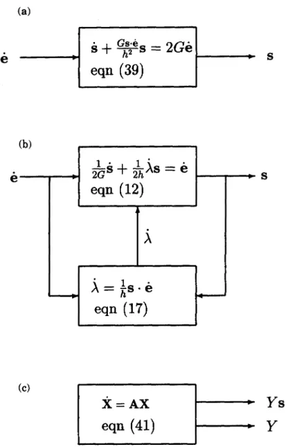
The block diagrams of Fig. 8 contrast three different points-of-view on the underlying structure of the on phase, Fig. 8(a) adopting the viewpoint of input-system-output in which the system is nonlinear, Fig. 8(b) also adopting the viewpoint of input-system-output but with output feedback (i.e., returning stress s) and state feedback (i.e., compensating with the intrinsic measure rate A), while Fig. 8(c) adopting the viewpoint of state equation in which the state vector is the internal state variables Ys and Yh (i.e., stress s and the intrinsic measure Y), and the state matrix is symmetric, traceless, singular, degenerate, and consists of the strain rate & and the intrinsic pseudo-relaxation measure G/h. It is observed that the implicit linearity is unfolded at the expense of raising one dimension up, and it looks linear in the extended state space and is not completely instantaneous. Thus we have revealed the

4292

(a)

H.-K. Hong and C.-S. Liu

ic=AX

ew

(41)

I

Ys Y

I J

Fig. 8. Superposition in the on phase explained by block diagrams: (a) nonlinear equation, (b) feedback system, (c) linear state equation.

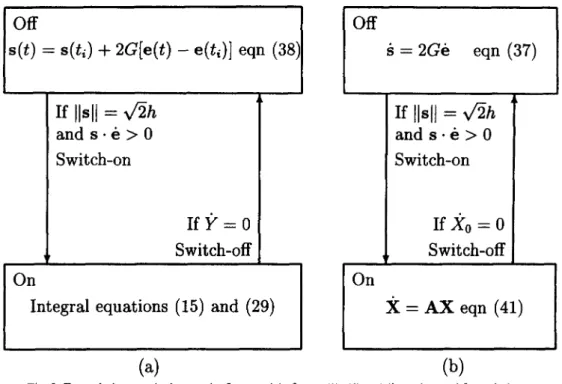
linearity of the Prandtl-Reuss model both in the on and off phases. It is described by a system of linear algebraic eqns (38), (or, equivalently, the differential eqns (37)) during the off phase, but governed by a system of simultaneous linear differential eqns (41) with variable coefficients (or, equivalently, by the consecutive linear integral eqns (29) and (15)) in the on phase. Indeed, it is a two-phase linear system with an on-off switch, as summarized diagrammatically in Fig. 9.

6. SWITCH-ON TIME

In this section and the following one we devote ourselves to a more global (temporally global) problem, namely to investigate when a given input of strain history switches plasticity mechanism on and off.

For an initial stress s(t,) which satisfies the inequality (4) and a strain history starting from the initial strain e(ti), the switch-an time can be determined according to the criterion (19) as follows. First solve for t the following algebraic equation

4293

s(t) = s(tJ + 2G[e(t) - e(ti)] eqn (38)

If llsll = &!h and s . k > 0 Switch-on A If%0 . Switch-off On

Integral equations (15) and (29)

Off i = 2Gci ew (37) If [IsI/ = fib and s . ti > 0 Switch-on I

I

If&O Switch-off On % = AX eqn (41)

(4

(b)

Fig. 9. Formulations equivalent to the flow model of eqns (l)-(6) : (a) linear integral formulation, (b) linear differential formulation.

&S(ii) ‘s(ti)+

kS(ti)’

[e(t) -e(h)] +[e(r) -e(ti)] * [e(t)--e(tJ] =

$,

₍₄₇₎

which is obtained by substituting eqn (38) into the yield condition s(r) * s(t) = 2h2. However, the solution t of eqn (47) must satisfy s(t) *e(t) > 0 in order to be the switch-on time t,,,. If there exist no solutions to eqn (47) or the solution t to eqn (47) does not satisfy s(t). c(t) > 0, then the strain path will not switch on the plastic mechanism.

7. SWITCH-OFF TIME

The task in this section is to determine the switch-off time t,such that Y(r& = 0 but Y(t) > 0 for all 5 E [ti, t,,,), given a strain history. Accordingly, we have to solve for t the following functional equation

f(t)

=z

Y(ti)S(ti)*e(t)+

$

s

‘e(t)*&(c)Y(t)d< = 0; 1;

(48)

the switch-off time tofl is the smallest t > ti which satisfies the above equation.

Next, we give an estimate of bounds on the switch-off time tQF Instead of eqn (48) one may solve the following lower and upper bound equations :

&S(t,) -b(t) +k(t) * [e(t) -C?(ri)] = 0, ₍₄₉₎

&S(lJ

‘e(t) +k(t) * [e(t) -e(tj)]p(ti, tb) = 0, ₍₅₀₎ which are obtained by nullifying Y,(t) and YJt) of eqns (35) and (36) respectively. The lower and upper bounds on the switch-off time f,,rare the smallest t > ti which satisfy eqns (49) and (50), respectively.

4294 H.-K. Hong and C.-S. Liu

An-example illustrating the determination of t,, and toff for a particular path will be given later in Sections 9.4 and 9.5, respectively.

8. SUPERPOSITION FORMULAE

In this section we explore the superposition principle [cf. Anderson et al. (1982)] for the Prandtl-Reuss model, starting from the nonlinear tensorial eqn (39). Assume s, to be a particular solution, satisfying

so

+

-so Gs,*l! = 2Ge.

h2 (51)

Then the time derivative of the following complementary solution

x:=s-ssg

₍₅₂₎

with the differential terms replaced by eqns (39) and (51), yields

G Gx-i!

k= ---[(SO.L)I+So@e]X--X

h2 ’ (53)

in which I is the fourth order identity tensor, Ix = x, and @ denotes the tensor product, (srJ 0 e)x = s&*x).

The equation adjoint to eqn (53) is

G G

p = -[(so -&)I+& @ s,]y- -6.

h2 h2

So the projective map

X

z:=---

1 +y*x

(54)

indeed supplies a linear homogeneous equation for z by using eqns (53) and (54) :

i=

-~[(s,~C)I+s,Oe]Z.

h2 Equation (55) can be inverted to

(56)

z

x==.

It is more convenient to eliminate y * x and y * z from eqns (55) and (57). Let

Vl := y-z, v2:= y-x.

Straightforward manipulation gives

(57)

4295 G 3, = --2.6, h* G $2 = --(I +v,)x*e. h2

The integrations of the above two equations yield

Thus we obtain G ’ v, =y*z= -- h’

s

z*de, v2 =y-x= -l+exp(-srx*de). z = xexp (s[x*de), Z x=

l+$

‘z-de s (59)

(60)

(61)

(62)

(63) (64)

from eqns (55) and (57).

We can now write a linear superposition law for z satisfying eqn (56) :

5

z = c ckzk, (65)

k=l

in which ck, k = 1, 2, 3, 4, 5, are constants and zk, k = 1, 2, 3, 4, 5, are linear independent solutions of eqn (56). The superposition law for z can be transformed to a superposition law for s as follows : substituting eqn (65) into eqn (64) and using eqn (63) for zk, we obtain

The integral term can be integrated out so that

J /

(66)

(67)

4296 H.-K. Hong and C-S. Liu s=so+ 1-i ck+ i k= I k=l c,exp (;r(sk-sO).de)’

(68)

where Sk, k = 0, 1, 2, 3, 4, 5, are the six independent particular solutions of eqn (38). Thus the formula (68) expresses the general solution of eqn (39) with ck, k = 1, 2, 3, 4, 5, determined by the five initial stress components s”(tJ, s22(ti), ?(tJ, s3’(ti), sr2(ti).

The superposition law (68) can be verified by another approach, starting from the linear matrix eqn (41), which has the general solution :

x = i

ckxk, k=O

in which ck, k = 0, 1, 2, 3, 4, 5, are constants and X P

k = 0, 1, 2, 3, 4, 5, are linear

independent solutions of eqn (41). Since a, a, - ~2~~2~ = 3/2 # 0, the relation (40) is invert- ible and therefore

Ys = i c, Yksk,

k=O (70)

Y=

5

ckyk.

k=O (71)

The above two equations can be combined to

ck yksk k=O

s= _{5 (72)}

1 CkYk

k=O

Because at the zero-value time Y(c,) = Y,(t,) = Y,(t,) = Y,(t,) = +. . = Ys(to) = 1 by eqn (14), it follows from eqn (71) that ZzCo ck = 1 or co = 1 -IE:=r ck. So the following super- position formula

s=

holds. Some manipulation gives

(73)

k$,

ck bk - sO) yk

s=s0+ ₍₇₄₎

Dividing both the numerator and denominator in the above equation by Y, and substituting

2 =

exp

(;I’(sk-.&de).

k = 1,2,3,4,5, (75)

which is obtained from eqns (14) and (17), we obtain eqn (68) again.

Comparison of the above two approaches leads us to conclude that the existence of the superposition formulae is attributed only to the implicit linearity no matter how they were discovered. The superposition formulae (68) and (73) are very enlightening, as will be demonstrated in the following section through a concrete example.

9. EXAMPLE: CIRCULAR PATHS

By a given input of strain history (resp. path) we mean either a prescription of the values of all strain components during a certain (finite or semi-infinite) time interval (resp. arc length), or specifying just part of strain components and allowing the other stress components which are conjugate to the unspecified strain components to be zero. The former may be given the specific name full strain control. However, the latter is more popular, for example, the strain controlled mode of a tension test.

9.1. Circular paths

In the sequel of this paper concentrate our study to a more following circular strain paths :

elI = oll +e,cosot,

we will for clarification and demonstration purposes specific class of histories, namely, the response to the

elz = o,* +eO sinot, s22 = s13 = s23 = 0,

ti,

s’

’

(a s12(ti) given, (76)

in which e, and w = 2n/T are, respectively, the amplitude and circular frequency of oscil- lation with T being the period of input, and o,, and on are constants denoting the center of the circular path. Whereas e(t,) is the prestrain, s(ti) is the prestress. One of the application areas of the paths is to study 90” out-of-phase cyclic effect. Note that at in eqn (76), and in due places which follow, may be replaced by w(t-ti) +& to more flexibly account for the initial phase &at the initial time ti. However, the replacement will not increase generality, since translating the time axis such that t, is adjusted to an appropriate value can also account for the initial phase.

For the paths, the second, third and fourth rows of e n (41) give e22 = ti,, = k3, = 0 if taking8=rr/6sothata,=1,a2=1/2,a3=Oanda,= _{P 3/2. Deleting vanishing rows and} columns, we have X = [A’, X2 X0]’ := y[s” s” h]’ ₍₇₇₎ and

!

0 0 A:=cio 0 0 ₍₇₈₎ -sinwt cosot where 2Ge, a:=--- h (79)

is the amplitude ratio, with a < 1, = 1, > 1 signifying the amplitude below, equal to and greater than the yield strain. Consequently, eqn (41) becomes

4298 H.-K. Hong and C-S. Liu _P, = -awX, sin it,

xi, =

aoX(J coswt:

X0 = a~(-X, sinwt+X,coswt).

(80)

(81)

(82)

9.2. Stress responses

After some operations on the above three equations, we find that

x6’“‘+(1 -L?)e_K& = 0, ₍₈₃₎

where the superscript (iii) stands for the third order time derivative. If the particular solutions of the above equation is obtained, the particular solutions of X, and X, can be calculated straightforwardly by eqns (80) and (81). Accordingly, we have the following fundamental matricest of eqns (80)-(82) :

(a) For a smaller amplitude, a < 1,

1

G?COSWt u cos(m + 1)ot 2(m+l) +

crcos(1 --m)wt ccsin(1 +m)wt a sin( 1 - m)wt -

2(1-m) 2(1+m) 2(1-m)

1

u=

a sin wt asin(1 -m)wt asin(1 +m)ot acos(1 -m)wt a cos(m + 1)wt . 2(1-m) + 2(1 +m) 2(1-m) - 2(m+ 1)

1

l

cos mot sin mot ₁

(84) (b) For the critical amplitude, a = 1,

coswt wtcosot-sinwt

I

- 2wt sin ot + (01’ t* - 2) cos cot

U = sinot cosot-totsinot 20tcosot+(w2t2-2)sinwt ₁ . ₍₈₅₎

(c) For a larger amplitude, a > 1,

r-

acoswt $(msinwt-cosot) ~(msinwtfcoswt)

u=

asinot ~(mcos~tfsinwt) T(-mcoswt+sinwt) ’ (86)

1 e InWl e --mu,

Here

m := Jm. (87)

The state transition matrix G(t, ti) is then evaluated by

G(t, ti) = U(t>U-’ (ti). 63)

Upon finding the state transition matrix G, the solution of X can be expressed as in the following :

7 The definitions and usage of a fundamental matrix and the state transition matrix can be found in most books on the systems of ordinary differential equations.

Y(f)s”(t) = G”(f,ti)Y(t,)s”(t,)+G’*(f,tl)Y(li)s”(ti)+hG’~(t,ti)Y(ti),

Y(t)s”(r) = G2’(r, ti)Y(ti)s1’(ti)+G22(t,li)Y(li)~‘*(ti)+hG23(t, ti)Y(ti),

hY(t) = G3’(t, ri)Y(ti)s”(ti)+G,,(t, ri)Y(ti)s”(ti)+hG,,(t,ti)Y(ti), in which G, denotes the ij-element of G. The stress response can be calculated by

4299

(89)

(90)

(91)

s’ ’ (t) = hGll(ty ti)~"(ti)+hG,,(ty ti)s'2(ti)+h2G13(t, ti) G~I(?,

ti)s”(ti)+G32(t,

ti)S'2(ti)+hG33(t, ti)

’

P(t) = hG,‘(t, ti)S’2(ri)+hG22(t, ti)s”(ti)+h2G23(t, t,) G3’(trti)~“(ti)+G32(f,f,)~‘~(fi)+hG33(t,ti) ’ 9.3. Superposition of stresses

For two-dimensional strain paths, the superposition formula (68) reduces to

(92)

(93)

i ckexp (~S’(S*-SO)‘de)(Sk-sO) k=l

s=s0+

(1 -cl -cz)+ i Ck eXp ($[@k-SO) ‘de)’

(94) k=l

which asserts that the three particular solutions of stress s,,, sl and s2 can be used to generate the general solution of stress s. In particular, the three columns of U obtained earlier are three particular solutions of X, and therefore can be utilized to generate three particular solutions of stress by using eqn (77) as follows :

(a) CI < 1 :

her cos(m + 1)wt ha cos( 1 -m)wt

hcrcoswt so = ’ ’ 2(m+l)cosmwt+2(1-m)cosmwt hcrsinwt ’ S’ = i ha sin( 1 - m)wt ha sin( 1 + m)wt ’ 2(1-m)cosmwt + 2(1+m)cosmwt

1

L .s2 = r

1

hcc sin( 1 + m)wt hcl sin( 1 - m)wt 2(1 +m) sinmwt - 2(1-m) sinmwt hacos(1 -m)wt ha cos(m + 1)wt 2(1 -m) sinmwt - 2(1 +m) sinmwt (b) a = 1:

1

h(wt cos wt - sin wt) 1 (95) h(coswt+wtsinwt) h[2wtcos wt+ (w’t’ -2) sin wt] (96)

4300 (c) c1 > 1 :

H.-K. Hong and C.-S. Liu

h cos wt

’ ’

$cosWf-msinwf) $sinwr+coswt)

so =

hsinwt ’ s, =

$rcosor+sinor) _t(- m cos wt + sin ot)

Note that the particular solutions sl, s2, ~0 satisfy the governing eqn (39) with the path (76) substituted, but do not account for any initial condition.

Similarly, for two-dimensional strain paths, the superposition formula (73) reduces to

(1 -c, -c2)Yoso+cl YlSl

+c,

Y,s,

s=

(1-c~-cc,)Yo+c,Y,+c*Y2 ’ in which Y,,, Y, and Y, are the third row of U divided by h : (a) c1< 1:

Y, = cos mot

(b) a = 1:

yo+ y,=y, y2q.

(98) (99)

(100)

(c) a > 1 : - rnWI y*

2--

h ’ (101)

The two constants cO and c, in eqn (98) can be determined by solving the following simultaneous equations : s”(t,) = (lpcl -C2)YO(ti)sA’(ti)+cl Y,(ti)s:‘(ti>+C2Y2(ti)S:‘(ti) I (1 -Cl -C*)Yo(td+c, Y,(tJ+crY*(tJ ’ (102) s12(t,) =

(l-‘l

-C*)YO(ti)S~2(ti)SCI y~~ti>~12(~i)+~2Y*(fj)~~2(ti) , (1-cl-c2)Y~(ti)+ClY,(ti)+C2Y*(ti) . (103)

The results are

ClOC22 -C2oC12 Cl 1 C20 -C21C10 c, = ) c2= 9 Cl lC22 -C21Cl2 CllC22--C21C12 where (104) Cl0 ‘= Yo(ti)[bS”(tj)-SA’(ti)]*

(a) a*1 (b) a=1 (c) a>1

Fig. IO. Superposition of stresses for (a) smaller amplitude (a -c l), (b) critical amplitude (a = I), (c) larger amplitude (a > 1).

c*, :=c*o--

_{y~~ti~~S12~ti>~s12~ci>l~}

C22 '=C20- Y*(fr)[S”(ti)-S:*(ti)]. ₍₁₀₅₎

After substituting these results into eqns (98) or (94) we obtain the solutions of the stress components s”(t) and s’*(t) for the prescribed initial values s”(tJ and s’*(tJ. In this sense we have derived the formulae of superposition to generate the general solution of the stress response.

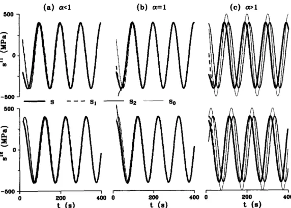
Figure 10 shows examples of the superposition of stress responses. In the calculations, G = 50,000 MPa, h = 400 MPa were taken. There provided three examples with different amplitudes :

(a) e, = 0.00397, c1 = 0.9925 < 1, smaller amplitude, (b) e, = 0.004, CI = 1, critical amplitude,

(c) e, = 0.005, CI = 1.25 > 1, larger amplitude.

Other data for the three inputs of circular strain paths (76) were prescribed identically as in the following : T = 100 seconds, ti = 0 second, (0, ,, 0i2) arbitrary, and the initial stresses s”(&) = s”(t,) = 0. The particular solutions sl, s,, so and the stress s obtained by using the superposition formula were all plotted in the figures. Being elastic so that eqns (94) and (98) are not applicable, the beginning portions of the curves of about ten more seconds? are not shown. Note that the phases of si, s,, s,, and s are different and that the amplitudes of the particular solutions sI, s2, s, are immaterial.

4302

9.4. Switch-on time

H.-K. Hong and C.-S. Liu

For the path (76) with initial stresses s”(ti) and d2(t,) satisfying the inequality (4), which is simplified to (s”)~+ (s’~)~ < h2, the switch-on time is determined by solving the following equation for t and taking the smallest t > ti:

b, cosut+b, sinot = bO, (106)

which is obtained by substituting eqn (76) into eqn (47) and in which

b, :=2cl

s’

h

’

(t,>

-Mcosux,

1

,

b2:=2c( P(fi) h-rsinwti

1

, 2 1 [ s’*(ti)

1

2 - __ h --sinoti .

Under the condition

the switch-on time t,, is found in Hong and Liu (1996a) :

1

- [ arcsin J& -arccosJ&:

1

ifb, 2 0, 0

to,

=

J& +arccosJ&:

1

ifb, < 0.

(107)

(109)

If the condition (108) is not satisfied, the circular strain path (76) never switches on the plastic mechanism [Hong and Liu (1996a)].

9.5. Switch-off time

As p(t) = 0, switching-off occurs, as specified by eqn (48). For the smaller amplitude case CI < 1, the switch-off time tqff is given by Hong and Liu (1996a) as

1

t o,f = t, + mw arctan rnJ=

b, (110)

For the other two cases a > 1, switching-off never occurs once already in the on phase, irrespective of prescribed initial stresses and the initial phase of the input circular strain path [Hong and Liu (1996a)].

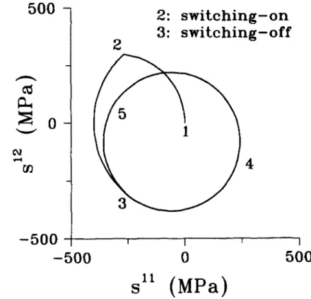
Finally, an example is given to illustrate the significance of the temporally global concept of switching-on and switching-off. All the data used in the calculations are the same as those used in Section 9.3, except herein e, = 0.003 (a = 0.75 < 1). For this the formulae (109) and (110) derived in the above give the switch-on time equal to 23.2 seconds

2: switching-on

2

3: switching-off

-500

500

8 (MPa)

Fig. 11, Stress response (12345345. .) to a strain input of periodic circular path.

and the switch-off time equal to 65.1 seconds (i.e., 0.651 cycle). Figure 11 shows the stress response path 12345345.. . , starting at point 1, switching on at point 2, then tracing 0.651 cycle of the yield circle, and switching off at point 3, from which on rotating around the smaller circle 345, which is tangential to the yield circle at point 3, around and around and never switching on again. Since the endless path 345345.. , is elastic while the preceeding arc 23 is elastoplastic, we say we have observed the phenomenon of shakedown. Before closing the example, it is interesting to note that the Prandtl-Reuss elastoplasticity has responded to an input of circular strain path by an output of piecewise circular stress path.

IO. CONCLUDING REMARKS

In this paper we have established three types of formulations for Prandtl-Reuss elastoplasticity : the axiomatized version of the flow model of eqns (l)-(6), the linear integral formulation in Fig. 9(a), and the linear differential formulation in Fig. 9(b). We have also discovered the superposition formulae (68) and (73), illustrating their usage. Only to the implicit linearity is attributed the existence of the superposition formulae no matter how they were discovered. The on-off switch of the mechanism of plastic irreversibility is indeed an indispensable part of a model of elastoplasticity. In this paper on the Prandtl- Reuss model we have exploited the meaning of the complementary trios (4)-(6), derived the on-off switching criteria (22) or (23), and posed the temporally global issues of switching-on and switching-off. The nature and profound content of the temporally global behavior can be further investigated in the framework of theories of dynamics and group, which will be presented in separate articles [Hong and Liu (1996a)].

Acknowledgement-The financial support provided by the National Science Council under Grant NSC 84-221 I- E-002-026 is gratefully acknowledged.

REFERENCES

Anderson, R. L., Harnad, J. and Winternitz, P. (1982) Systems of ordinary differential equations with nonlinear superposition principles. Physica 4D, 164-182.

4304 H.-K. Hong and C.-S. Liu

Hashiguchi, K. (1994) On loading criterion. Infernational Journal ofPlasficity 10,871-878.

Hill, R. (1958) A general theory of uniqueness and stability in elastic-plastic solids. Journal of the Mechanics and Physics of Solids 6, 236249.

Hill, R. (1967) On the classical constitutive relations for elastic/plastic solids. In Recent Progress in Applied Mechanics-The Fulke Odquist Volume, eds B. Broberg, J. Hult and F. Niordson. Wiley, New York, pp. 241- 249.

Hong, H.-K. and Liou, J.-K. (1993) Integral-equation representations of flow elastoplasticity derived from rate- equation models. Acta Mechanica 96, 18 l-202.

Hong, H.-K. and Liu, C.-S. (1993) Reconstructing J2 flow model for elastoplastic materials. Bulletin of the College of Engineering, N.T.U. 57,95-l 14.

Hong, H.-K. and Liu, C-S. (1996a) Dynamic system theoretic study of perfect elastoplasticity under circular generalized strain paths. In preparation.

Hong, H.-K. and Liu, C.-S. (1996b) Minkowski spacetime M”+’ and Lorentz group SO&, 1) of perfect elasto- plasticity. In preparation.

Il’yushin, A. A. (1963). Plasticity. Foundation of General Mathematical Theory. Akad. Nauk S.S.S.R., Moscow (in Russian).

Krieg, R. D. and Krieg, D. B. (1977) Accuracies of numerical solution methods for the elastic-perfectly plastic model. Journal of Pressure Vessel Technology ASME 99, 5 1 O-5 15.

Liu, C.-S. (1993) Theelastoplasticevolution and stability ofmaterials under mechanical and thermal environments. PhD dissertation, Department of Civil Engineering, Taiwan University.

Lubliner, J. (1984) A maximum-dissipation principle in generalized plasticity. Acta Mechanica S2,225-237. Ohashi, Y ., Tokuda, M. and Yamashita, H. (1975) Effect of third invariant of stress deviator on plastic deformation

of mild steel. Journal of the Mechanics and Physics of Solids 23, 295-323.

Prandtl, L. (1924) Spannungsverteilung in plastischen kcerpern. In Proceedings of the 1st International Congress on Applied Mechanics, pp. 43-54, Delft.

Reuss, E. (1930) Beruecksichtigung der elastischen formaenderungen in der plastizitaetstheorie. Zeits. angew. Math. Mech. (ZAMM) 10,266274.

Winternitz, P. (1982) Nonlinear action of Lie groups and superposition principles for nonlinear differential equations. Physica 114A, 105-l 13.