Ultrasonic sensor data integration and its application to environment perception

(1)

Ultrasonic Sensor

Data

integration

and

its

Appiicatiun

to

Envimmnt

Perception

. . .

Charles C. Chang Kai-Tai Song*

Department of Control Engineering National Chiao Tung University 1001 Ta Hsueh Road

Hsinchu 300, Taiwan, R.O.C.

Received October 14, 1994, revised November 13, 1995; accepted May 20, 1996

To move in an unknown or uncertain environment, a mobile robot must collect information from various sensors and use it to construct a representation of the external world. Ultrasonic sensors can provide range data for this purpose in a simple and cost-effective way. However, most ultrasonic sensors are not sufficient for environment recognition because of their large beam opening angles. In this article the beam-opening-angle problem is solved by fusing data from multiple ultrasonic sensors. We propose two methods for sensor data fusion. One uses an artificial neural network (ANN), and the other is based on a mathematical model. Simulations and experiments show that the mathematical model is more accurate when there is no noise in the sensor readings, but the ANN method is better when the sensors are subject to much noise. To extract line segments from the ultrasonic image, we develop a line extractor that is more efficient than traditional line fitting methods in this application. Experimental results show that this method is effective for environment perception in a robotic system.

0 1996 John Wiley 6- Sons, bic.

*To whom all correspondence should be addressed. Journal of Robotic Systems 13(10>, 663-677 (1 996)

(2)

1. INTRODUCTION

To enable a mobile robot to navigate in an unstruc- tured or frequently changing environment, it is necessary to apply sensors to recognize the environment. However, a single sensor provides only incomplete information about the environment. Since each sensor can take only a single type of observation over a limited range, information must be combined from many sensors. It has been shown that using more sensors will almost always improve the estimation.' A survey paper by Luo and Kay2 discussed various aspects of the problem of integrat- ing multiple sensors. Sensor fusion can be implemented on the data level,2 feature l e ~ e l , ~ - ~ or deci- sion l e ~ e l . ~ , ~ In this article, we develop a scheme for data level fusion of multiple ultrasonic sensors. From our results concerning data-level fusion, useful features can be extracted.

The sensors used in this article are ultrasonic sensors, which provide range data in a simple and cost-effective way. However, these sensors are not sufficient for environment perception, mainly because of their wide beam opening angle. Elfes used a probability-grid map to deal with sensor uncertainty. lo This method solved the beam-opening-

angle problem at the stage of sonar-mapping, but the grid itself is a source of uncertainty. Crowley estimated the object's direction using scanning data.'' This method is simple, but suffers from noise and cannot eliminate the beam-angle problem with only a couple of sensor readings. Nagashima and Yuta used a sensor system that consisted of one transmitter and two receivers to estimate the normal direction of walls.12 This method, however, uses an approximation in the estimate formula. On the other hand, Barshan and Kuc analyzed the physical model of ultrasonic sensors and derived a method that can estimate the inclination angle between the sensor orientation and the normal direction of a wall.13

The sensor fusion methods developed in this article eliminate the beam-angle problem with a single observation from a multi-sensor system. Our method does not limit the maximum incident angle of an ultrasonic wave to a plane. Therefore, if the plane to be detected is not mirror-like, our method will have a larger usable range than the methods

proposed by Barshan and Kuc13 and Nagashima and Yuta.I2 The next section describes the use of an artificial neural network (ANN) to find a better estima- tion of ultrasonic sensor images. In section 3, a math- ematical model is developed to solve the same problem, and its results are compared with those of the ANN method. After a good estimation of the distance measurement is found, a line-extraction algorithm is used to extract line segments. Although several line-fitting algorithms have been pro- they tend to be slow for ultrasonic im- aging because there are too many split operations (especially around corners) requiring too much re- calculation. We have developed a new line extractor, which will be described in section 4. Our conclusions are presented in section 5.

2. SENSOR DATA FUSION USING ANN

The ultrasonic range sensor is a time-of-flight system that gives a range value when the echo first exceeds a certain threshold level. The echo amplitude depends on the inclination angle of the returned wave. l3 Therefore, the sensor model can be simpli-

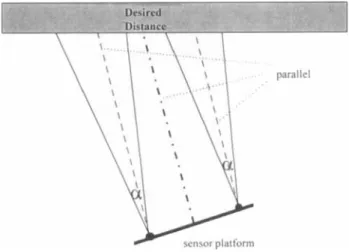
fied to detect the shortest distance to objects within a fixed beam opening angle. This simplified model was also used by Crowley." However, the ultrasonic sensor may not detect a plane because the wave reflects away for large incident angles. The maximum incident angle depends on the texture of the plane. For a wooden board, the maximum incident angle is about 22.5'; for a brick wall, it can be as large as 70". In the simulations in this article, we assumed the maximum incident angle to be 40". Al- though there is more sensory information in this case than in the case of a mirror-wall, the information is not accurate because of the beam-opening angle. As shown in Figure 1, when the sensor turns away from the normal direction, it reads the first returned echo caused by the side of the beam instead of the center. This leads to difficulties in understand- ing the environment. However, by examining the geometrical relation of the measured distance to the actual distance, we thought this problem could be solved by arranging multiple sensors at different lo- cations in different directions. The problem then be-

(3)

Chang and Song: Ultrasonic Sensor D a t a Integration 665

Figure 1. Measurement error due to beam opening angle of ultrasonic transducers.

comes that of mapping the geometrical relation between the raw sensor data and the desired distance. Such a mapping may be highly nonlinear and we have no specific way to follow to analyze it. In this case, it might be better to take advantage of the ANN, which is model-free and suitable for nonlinear mapping problems.

2.1. Design of ANN

An arrangement of the sensor platform is illustrated in Figure 2. We place two ultrasonic transducers on the platform so that their center lines are parallel. Each transducer works as a transmitter as well as a receiver. It transmits ultrasonic waves and receives its own returned echo. To prevent the waves from interfering with each other, the transducers are fired sequentially. These sensor readings are very often contaminated by the beam-opening-angle effect. To simplify the problem, it is assumed that the objects in the environment were of long-wall outline. Sensor readings from these two transducers are fused into the ANN for a better estimation of the actual distance. The inputs of the ANN are the two sensor readings. The output is the distance from the center of the sensor platform to the obstacle in the direction of the platform heading (see Fig. 2). The ANN adopted here is a feed-forward network trained by a back-propagation a1g0rithm.I~

In simulations, both one- and two-hidden-layer ANNs were tried. It was found that using a two- hidden-layer neural network was necessary because the mapping function might be complex. After several tests, it was determined that the ANN should use 25 processing elements for each hidden layer. The sensor data were generated by a model of the ultrasonic sensor with a beam opening angle of 22".

In this model, the reading of the sensor was assumed to be the shortest distance from the sensor to the obstacle within that angle. The effective range of the sensor was from 0.3 to 4.5 m. The training data were randomly generated within the effective range and with the incident angle varying between 0" and 40" (because of symmetry, the results can be extended to the angle between 0" to -40"). The whole set of training data for the ANN consisted of two thousand sets of sensor readings. Initial weights were set between 1.0 and - 1.0 randomly. During the training,

every item of training data was put into the ANN and then the weights were adjusted iteratively. All the training data were used cyclically until the output error of the ANN converged. Because the initial weights might affect the results due to the local error minimum problem, several sets of initial weights were tried.

We noticed that the ultrasonic sensor does not suffer from the beam-opening-angle problem around the zero incident angle. Therefore, around the zero incident angle it is better to use a single sensor than to have the readings be processed by the ANN, which only obtains a good approximation. The ANN actually can learn well around zero incident angle, but we just should take advantage of the ultrasonic sensor characteristics. Because our sensor system has no transducer at the center of the platform, where the desired distance was measured, we used the average of the two sensor readings to estimate the desired distance around the zero incident angle. For larger incident angles, ANN fusion is still useful for obtaining a reliable estimate. For clarity, we call this method partial ANN fusion to distinguish it from pure ANN fusion.

(4)

I I 1 I

0

0 100 200 300 400 5

Epoch

Figure 3. Learning curve of ANN

2.2. Simulation Results for ANN Fusion

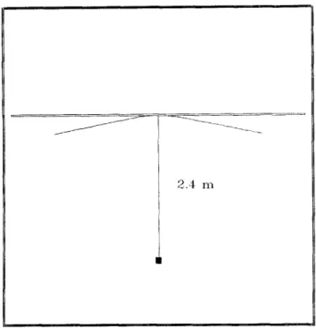
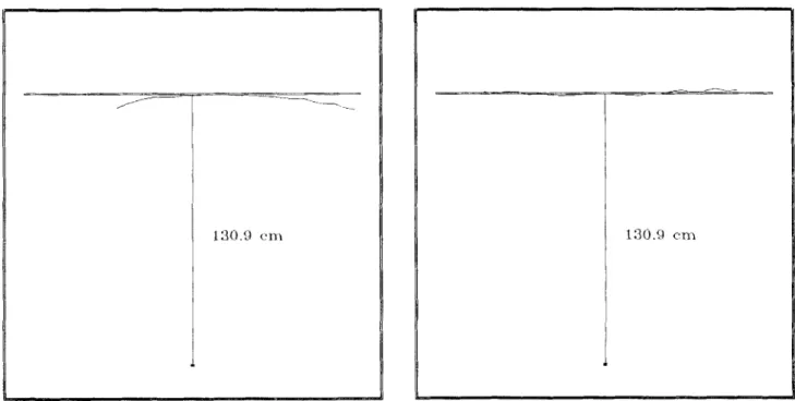
Figure 3 shows the learning curve of the ANN. The learning was fast in the beginning, then it slowed down and took much time to achieve the minimum error state. We demonstrate the mapping results by scanning a flat wall. Figure 4 shows the simulation results. In Figure 4(a), a single sensor cannot pro- duce good scanning results because of the 22" beam angle. Figure 4(b) is the scanning result obtained by applying pure ANN fusion. This result fits the actual wall well. Comparing Figure 4(a) and Figure 4(b), we find the so-called "around zero" incident angle is the incident angle smaller than about 5.7". We derive the following criterion to identify this situa- tion in the raw sensor data:

where d , and d2 are the two sensor readings. The value 3 cm is the difference between the distance of the two sensors to the wall when the inclination angle is 5.7" and the distance between the two sensors is 30 cm. As described in the previous para- graph, we take the average of the two sensor readings in this case, instead of applying ANN fusion. Figure 4(c) shows the result obtained by using the partial ANN fusion. It is obvious this result is better

than that of the pure ANN method around the zero incident angle.

2.3. Experimental Results for ANN Fusion

A practical test was carried out in the laboratory to

verify this sensor fusion method. We installed two Polaroid ultrasonic sensors in parallel on a platform that could be rotated by a step motor. The system was programmed to scan a flat wooden wall ahead of it. The measured range data were taken every 1.8". Figure 5(a) shows a scanning image from the right-side sensor. The sensor data near the middle of the wall (around the zero incident angle) are still good. This is because the beam-opening-angle problem does not occur here. It also shows that the raw sensor data were contaminated by noise. Figure 5(b) shows the result with the partial ANN fusion. An obvious improvement can be observed in the fusion result.

3. FUSION USING A MATHEMATICAL MODEL

Although we hypothesized that there existed a geometrical relation between the data of the two sensors and the desired estimation, this relation was not

(5)

Chang and Song: Ultrasonic Sensor Data Integration 667

2.4 r n

However, after careful examination, we also derived a mathematical formula as described below.

The difference between the readings of the two sensors (see Fig. 6) is

where d, and d, are the sensor readings and 6,, is the difference in the distance indicated by the two sensors. The incident angle I3 can be calculated with 6, by the law of cosines and the law of sines. Assume

I3 z -, as shown in Figure 6(a). Then one can first calculate 8 by

ff 2

and

~

Figure 4(a). Scanning image of single sensor.

(4)

8 d -

Y

--

sin I3 sin(n-/2 - ai2)

obvious and we did not have a known procedure to follow for mathematical analysis. Therefore, the ANN method, which is model-free and suitable for mapping problem, was first applied to this problem.

where

x

is the distance between the two sensors and

a! is the beam opening angle. If the calculated 0 is

greater than -, ff then it is correct (to be proved in the 2

Figure 4(b). Scanning image after pure ANN sensor fusion.

Figure 4(c).

fusion.

(6)

Figure 5(a).

gle sensor.

Experimental result of scanning image of sin-

Appendix) and the desired distance D is d,,, C O S ( ~ - (~12)

D =

cos 6 (5)

where do,, is the average of d , and d,.

If the calculated 6 is not greater than ?, then 6' is smaller than

-

(see the Appendix), as shown in Figure 6(b). The 6 should be re-calculated by

2 a 2 X - sin6 sinn-12 '

The desired D is then

To cope with noise, more sensors can be added without causing much extra computational load. For example, if a five-sensor system is used, then

Figure 5(b). Experimental result of scanning image after

partial ANN sensor fusion.

I (13)

d,

+

d ,

+

d3

+

d4

+

d5 5

daw =

where d,

,

d,, d 3 , d,, and d , are the readings of the five sensors. If is used instead of 6, in the previous formulation, the desired D can be calculated out the same way. Because and d,,, are the average of multiple data, the noise is also averaged and so the effect of noise is reduced. Figure 7 shows experimental result of a test using the mathematical model. The mathematical model yields even better fusion results.

3.1. Comparison of ANN Method and Mathematical Model

To compare the above sensor fusion methods, we define the fusion error of an observation as the real normal distance from the sensor unit to the wall

minus the average normal distance of the estimated data. We also investigated the effect of noise on the

(7)

Chang and Song: Ultrasonic Sensor Data Integration

669

a

Figure 6(a). Mathematical model: 6 2 -.

2

distance

Y

sensor platform --c/

Figure 6(b). Mathematical model: 6 < E,

2

fusion methods. Ultrasonic sensor data sometimes contain Gaussian noise. There are two kinds of noise: in the first, the standard deviation is proportional to the distance that the wave has travelled; in the sec- ond, the standard deviation is fixed. In a harsh envi-

ronment, the noise can be on the order of a few percent. For example, temperature is a predominant noise source. There is 3.5% difference in ultrasonic sensor measurements when the temperature is 5" C and 25" C.

(8)

Figure 7.

sor fusion by mathematical model.

Experimental result of scanning image after sen-

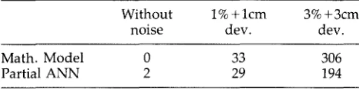
Table I and Table I1 summarize the mean error and the mean square error of the simulations. For simulation with noise, the error in the tables is the average value of several trials. From Table I, it can be seen that the mean errors are almost equal. How- ever, from Table 11, we find that when noise is absent the mathematical model is of zero mean square error and better than the ANN method. When the noise is of 1% distance-proportional standard deviation plus 1 cm standard deviation, the two methods per- form almost equally well. When the noise is in- creased to have 3% distance-proportional standard deviation plus 3 cm standard deviation, the ANN method has much less mean square error than the mathematical model. The less mean square error, the more likely to distinguish whether two data are from the same feature. Therefore, one can obtain better feature-level information with the ANN fusion

Table 1. (unit: cm).

Comparison of methods in terms of $d,ilur

Without 1% +lcm 3% +3cm

noise dev. dev.

Math. Model 0 0 5

Partial ANN -1 -1 4

Table II.

(unit: cm2).

Comparison of methods in terms of $:,,,,

Without 1 % + l c m 3%+3cm

noise dev. dev.

Math. Model 0 33 306

Partial ANN 2 29 194

data when the sensor data contain excessive noise. The anti-noise capacity of the ANN method is ex- plained below. Under the larger noise circumstance, many input patterns are out of the work space. For the ANN method, it learns to generalize the mapping for the interested operation space. If an input pattern is a little beyond the work space, it will be mapped to a value close to the desired one because of the generalization property of ANN. However, the mathematical model will always give an answer no matter how inappropriate the input pattern is. This will result in a large deviation. In conclusion, the mathematical model is better for a small noise environment, while the ANN method is more suitable for an environment with large noise. For the environment of the previously shown experiment, the two methods give practically the same results, as shown in Table 111.

4.

LINE EXTRACTOR FOR

ENVIRONMENT PERCEPTION

It is very often desirable to represent the environment using high-level features such as the edges of objects. In this article, only two-dimensional representation is considered. The previous fusion results can be used to extract lines that are the edges of objects. The line-fitting or line extraction methods have been paid much attention for the last decades because of the development of vision systems. In the vision field, Hough transform is the most often used method for line extraction.I6 This method is,

Table 111. Experimental results for different methods.

Math. Model 0.5 0.8

(9)

Cliang and Song: Ultrasonic Sensor D a t a Integration 671

however, computationally time-consuming. Sup- pose each axis of the parameter space of Hough transform is quantized into K values (this quantiza- tion also limits the precision of results) and there are n image points, then nK computations are required. For our ultrasonic fusion results, a line is apparently constituted by the neighboring points in the data set, which is different from the case in vision data. Accordingly, we developed a faster method which needs only n computations. Our line extractor is based on the basic line-fitting f0rmu1a.l~ Suppose the line equation is expressed as

and

s,

=

2 xi

% (24)

In addition, the variance of these points relative to the line is

Then we have

e, = /sin

.

x,

-t- cos

4 .

y, - dJ, ₍₁₅₎ where e, is the Euclidean distance between

(x,,

y,) and the line. Define the error norm

E,

for a point set S , to the extracted line as

where

E,

can be expressed as

E,

=

2

e;.

Sk

4.1. Application to Feature Recovery

In previous sections, the system obtains estimated distances from the mobile robot to obstacles by sensor fusion models. These distances are derived from sequential scanning readings. The system then transforms these distances into point positions. These points are also in sequential order, and the line-extracted algorithm is applied to them. First, we determine the parameters

q ,

s:, and no. The parameter n, is the minimum number of points that construct a line with s:

<

s:, which is the limit of the acceptable s3 value. The parameter no determines the extent of an outlier. The choice of these parameters depends on the type of sensor and the environment. For the scanning image after the fusion of ultrasonic sensors, we chose n, as 10 (covers 18"),

sf

as 0.0004 m2, and

12, as 3. Let the system start with the first point in

the raw data memory. Then the procedure can be summarized as follows:

The best approximate line can be defined as the line minimizing E,

.

To calculate the approximate line equation, we can use the following formula:

where, if there are N k points in S,,

s,

v

- - - N k

s2,

vx,

=

s,,

- - N k

1. Put the izl consecutive points from memory

into a new data set, and find the fitting line equation and the corresponding variance. If s ; < s f , then this data set constructs a line and continue to step 2; else, remove the first point in the data set and add the next point

sx

S Y

v,,

=

s,,

- __

(10)

from memory into the data set, then repeat this step.

2. Check whether the next point is an outlier or not. The checking method is as follows: Suppose the next point is ( x i , yi) and the line equation determined earlier was

(31) sin

C#Ik

-

x

+

cos (bk.

y

= d.

We will have error ei

If ei is larger than nos,, then the system con- cludes the point

(xi,

yi)

is an outlier. If the point is an outlier, the previous line segment ends up at the last point and go to step 1; else, put this point into the data set and go to step 3.

3. Find the new extracted line for the new data set. If s:

<

s:, then the new equation for the line is acceptable and go to step 2; else, the line segment ends up at the last point and go to step 1.

These steps are repeated until all points in memory are processed. The system will find the line segments in the environment.

After the lines are extracted, an operation of line combination will still be needed because adjacent lines separated by outliers may be on the same line (edge). If the parameters ($ and d) of the equations of the adjacent lines differ only by a small value, the new line equation will be re-calculated for the points used to construct the original line segments.

Comparing our method with the conventional method such as proposed by Pavlidis and Horo- witz,14 we find their method requires much re-calculation because many erroneous data in the ultrasonic image lead to many iterations of split-and-merge operations. This means some data points should be calculated many times for checking if a split is needed. In contrast, in the method we proposed, each data point is considered only once. Although in our method the line equation should be calculated every time a point is added to a line, the core compu- tation ((24)-(28)) can be updated easily. Therefore, our method will be more efficient for ultrasonic measurements. For a mobile robot to navigate in an un- structured environment, this increase in efficiency will be very important for real-time performance of dynamic map building.

4.2. Experiment on Environment Perception

In this experiment, the feature recovery capability of the sensor system was tested using the line extractor. The experiment was implemented in a room with four walls. The position of the sensor system was at the origin, and the four vertices of the walls were at (-1.28 m, -0.85 m), (0.79 m, -0.84 m), (0.71 m, 0.73 m), and (-1.35 m, 0.73 m). Each wall was con- structed either of wooden board or of cartons. Be- cause the environment was closed, the recognition of the environment could be realized by connecting the lines extracted by our algorithm. (However, if the environment to be detected is not closed, we can use other sensors to determine the end points of a line or integrate observations from different scanning points.) The sensor system was the same as that described in the previous section. Figure 8 is the scanning image using only one sensor. In this figure, there are erroneous data at the right side and there are some specular reflections around the corner. Because of the beam-opening angle and multiple reflection, the lines extracted from the single sensor data do not match the environment well (see Fig. 9).

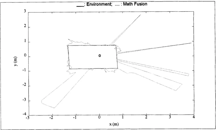
The fusion result using the ANN method is presented in Figure 10. This result shows a better estimation around the small incident angle, while the erroneous data area is more uncertain. This type of result helps the line extractor find the correct lines and estimate them more accurately. This is because when the erroneous data are amplified, they will not be misjudged as correct ones. Therefore, the extracted line will not be contaminated by the erroneous data. The result of applying the line-extracted algorithm is shown in Figure 11. In this figure, lines are extracted around the small incident angles, where there are many scanned data points that are linearly distributed. Although it seems a line exists in the lower-left area, there are only about 7 points in that region, which are not adequate to extract a line. As described previously, at least 10 data points are required to extract a line in our algorithm. The result shown in Figure 11 is more acceptable than that in Figure 9. A similar result was obtained by using the mathematical model to fuse the sensor data. How- ever, since the effect of noise was not serious, the mathematical model produced a better fusion result (see Fig. 12, especially around the small incident angle). Therefore, the features recovered from its scanning image were more accurate (see Fig. 13). Figure 14 summarizes the features recovered from

(11)

Chang and Song: Ultrasonic Sensov Data integration 673

-

: Environment;

....

: One Sensor

3 2 1 0 -1 -2 -3 -4

Figure 8. Scanning image of single sensor for a room.

-

: Environment;

....

: Feature from One Sensor

h W

E

x 1 , . I I 0.8 - 0.6 - 0.4

-

0.2 - 0 - -0.2 - -0.4 - -0.6 - -0.8 - 0 I I -1.5 -1 -0.5 0 0.5 -1 x (m>

(12)

- ... ... ... ... 1 : - - - 0

-

- - - - ... ... ,. ... I I I I -1 -0.5 0 0.5 1

-

:

Environment;

....

:

A N N

Fusion 3 2 1 0 -1 -2 -3 -4 ... .. ...-... ....

Figure 10. Scanning image after ANN fusion for a room.

-

:

Environment;

....

: Feature from

A N N

Fusion

n ;h

E

v 1 0.8 0.6 0.4 0.2 0 -0.2 -0.4 -0.6 -0.8 -1 -1.

(13)

Chang and Song: Ultrasonic Sensor Data Integration 675

-

: Environment;

....

: Math Fusion

n

E

v h 3 2 I 0 -1 -2 -3 -4

Figure 19. Scanning image after sensor fusion by mathematical model for a room.

n v E h 1 0.8 0.6 0.4 0.2 0 -0.2 -0.4 -0.6 -0.8 -1 -1

-

: Environment;

....

: Feature from Math Fusion

0

I I 1 I

-1 -0.5 0 0.5

x

(4

-

(14)

-

: Environment;

_._._

: Of One Sensor;

_ _ _

: Of ANN;

....

: Of Math 1 0.8 0.6 0.4 0.2 v

B

o

h -0.2 -0.4 -0.6 -0.8 -1 -1 0

Figure 14. Features recovered using various scanning images.

different scanning images. These results indicate our fusion methods and the line extractor are effective.

5. CONCLUSIONS

In this article, we propose two methods for the fusion of ultrasonic sensor data, one based on the

ANN

structure and the other on mathematical analysis. The mathematical model is suitable for situations with little noise, while

ANN

fusion is more suitable for cases with much noise. Both methods yield acceptable results.

A

line-extraction algorithm is developed to extract line segments efficiently. It is more efficient than the traditional line fitting method because it does not use repeated split and merge operations, which are often needed with ultrasonic images. Therefore the proposed method is effective for environment perception.

One limitation of the proposed methods is that the end points of a line segment cannot be identified when the environment is not closed. We have not yet considered how to detect the corners in this article. In our future work we will attempt to find a

fusion scheme to identify corners, and to use other types of sensors to compensate for the limitations of the ultrasonic sensor.

The authors are grateful for valuable suggestions from the referees. This work was supported by the National Science Council, Taiwan, ROC, under contract NSC81-0404-E-009-022.

APPENDIX: PROOF OF ANGULAR CONDITIONS IN THE MATHEMATICAL MODEL

We stated that if we first assume 8 z - ff and calculate 2

8 by (3) and (4), then if the calculated 8 2

-

a it is .

correct; if the calculated 8 is smaller than -, ff we con-

2 ’ 2

clude that 8 is actually smaller than and must be re-calculated by (6). To prove this statement, we note, in Figure 6(a), that

(15)

Chang and Song: Ultrasonic Sensor Data Zntegration 677 where /3 can be derived from

x,

y, and S d . The H

calculated from this equation is exactly the same as that from (4). Denote the real 6, by 6, and the H calculated from ( 3 ) and (33) by 6 . Then

(34)

a a

d r 2 - I + H = $ > -

2 I - 2

If 6'

<

d 2 , e uation (6) holds. However, if (3) and

(337 are used% find 8, the

y

calculated from (3) is erroneous and then

p

is not equal to -. Comparing (6) and (33), we have T 2 a H , < - + H < d , . < E . 2 2

(Note: The range of 6 is from 0" to 90".) From (34) and (35), we have

(35)

(37)

a CY

Therefore, if 0 2 -, then H > -, so 0 is correct. It,

2 ' - 2

otherwise, H

<

-, then 6,

<

- and 6 is wrong, so it needs to be re-calculated by (6). Obviously, the statement holds. Similarly, we can prove it is proper to assume H

<

first when using the mathematical model to find

D.

a a

2 2

2

REFERENCES

1. J . M. Richardson and K. A. Marsh, "Fusion of multi- sensor data," lnt.

1.

Rob. Res. 7(6), 78-96, 1988.

2. R. C. Luo and M. G. Kay, "Multisensor integration and fusion in intelligent system," I E E E Trans. Syst. Man Cybern., 19, 901-931, 1989.

3. H. F. Durrant-Whyte, "Consistent integration and propagation of disparate sensor observations," lnt.

1.

Rob. Res., 6(3), 3-24, 1987.

4. P. L. Bogler, "Shafer-Dempster reasoning with applications to multisensor target identification systems,"

l E E E Trans. Syst. Man Cybern., SMC-17,968-977,1987.

5. I. J. Cox and J. J. Leonard, "Probabilistic data associa- tion for dvnamic world modeling: A multiule hvuothe- sis approach," Proc. ICAR, &a, Italy: 19%, pp. 1287- 1294.

6. C. Ferrari and G. Chemello, "Coupling fuzzy logic techniques with evidential reasoning for sensor data interpretation," Puoc. liitell. Auton. Syst.-2, Amster- dam, Netherlands, 1989, pp. 965-971.

7. L. I. Perlovsky and M. M. McManus, "Maximum likeli- hood neural networks for sensor fusion and adaptive classification," Neural Networks, 4, 89-102, 1991. 8. B. J. Thien and S. D. Hill, "Sensor fusion for automated

assembly using an expert system shell," Proc. ICAX,

Pisa, Italy, 1991, pp. 1270-1274.

9. K. T. Song and J. C. Tai, "Fuzzy navigation of a mobile robot," in F L ~ Z Z ~ Logic Tecknology and Applications,

R. J. Marks 11, Ed., IEEE Press, New York, 1994, pp. 141-147.

10. A. Elfes, "Sonar-based real-world mapping and navigation," I E E E Trans. Rob. Autoin., RA-3,249-265,1987.

11. J. L. Crowley, "Dynamic world modeling for an intelligent mobile robot using a rotating ultrasonic ranging device," Proc. l E E E l n t . Conf. Rob. Autoin., St. Louis,

12. Y. Nagashima and S. Yuta, "Ultrasonic sensing for a mobile robot to recognize an environment," Proc. lEEEiRS1 IROS, Raleigh, NC, 1992, pp. 805-812.

13. B. Barshan and R. Kuc, "Differentiating sonar reflections from corners and planes by employing an intelligent sensor," l E E E Trans. Pattern Anal. Mach. lntell,,

12(6), 560-569, 1990.

14. T. Pavlidis and S. L. Horowitz, "Segmentation of plane curves," l E E E Trans. Comput., C-23, 860-870, 1974.

15. P. K. Simpson, Artificial Neural Systems, Pergamon

Press, New York, 1990.

16. E. R. Davies, Machine Vision: Theory, Algorithms, Practi-

calities, Academic Press, London, 1990.