Item 987654321/15891

全文

(1)A Process Pattern Mining Framework for the Detection of Health Care Fraud and Abuse. A Thesis Submitted to the Faculty Of National Sun Yat-sen University By Wan-Shiou Yang. In Partial Fulfillment of the Requirements for the Degree Of Doctor of Philosophy. June, 2003.

(2) TABLE OF CONTENTS. ABSTRACT… … … . . . … … … … … … … … … … … … … … … … … … … … … … … … v LIST OF FIGURES … … … … … … … … … … … … … … … … … … … … … … … … … .vi LIST OF TABLES … . … … … … … … … … … … … … … … … … … … … … … … … … viii. 1. Introduction… … … … … … … … … … … … … … … … … … … … … … … … … … … 1 1.1 Motivation… … … … … … … … … … … … … … … … … … … … … … . … … … 1 1.2 Problem statement and the proposed approach… … … … … … … … … … … … 2 1.3 Overview of the research… … … … … … … … … … … … … … … … … … … … 3. 2. The Problem and the related work … … … … … … … … … … … … … … … … … … 4 2.1 Health care fraud and abuse … … … … … … … … … … … … … … … … … … … . 4 2.2 Current status… … … … … … … … … … … … … … … … … … … … … … … … … 8 2.3 Clinical pathways… … … … … … … … … … … … … … … … … … … … … … … . 9 2.4 Research framework … … … … … … … … … … … … … … … … … … … … … ...15. 3. Structure pattern discovery… … … … … … … … … … … … … … … … … … … … … .18 3.1 Related works… … … … … … … … … … … … … … … … … … … … … … … … .19 3.2 Formalization of structure pattern discovery problem… … … … … … … . . . … 2 0 3.3 Structure pattern discovery algorithms… … … … … … … … … … … … … … 2 3 3.3.1 TP-Graph algorithm… … … … … … … … … … … … … … … … … … … 2 3 3.3.2 TP-Itemset algorithm……………………………………………...…34 3.3.3 TP-Sequence algorithm……………………………………………...36 3.4 Performance evaluation… … … … … … … … … … … … … … … … … … … … 4 1. ii.

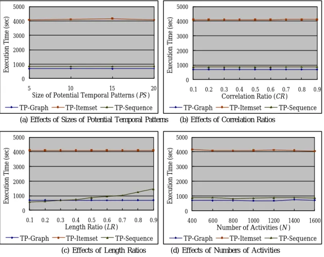
(3) 3.4.1 Generation of synthetic data… … … … … … … … … … . … … … . . . … . 4 1 3.4.2 Effects of minimum support thresholds… … … … … … … … … … … 4 3 3.4.3 Effects of instance characteristics… … … … … … … … … … … … . . . … 4 5 3.4.4 Scale-up experiments… … … … … … … … … … … … … … … … … … 4 7 3.5 Summary… … … … … … … … … … … … … … … … … … … … … … … … … … 4 9. 4. Feature selection… … … … … … … … … … … … … … … … … … … … … . … … … … 5 0 4.1 Related works… … … … … … … … … … … … … … … … … … … … … … … … 5 1 4.2 Formalization of feature selection problem… … … … … … … … … … … … .53 4.3 Feature selection algorithms… … … … … … … … … … … … … … … … … … 5 7 4.4 Performance evaluation… … … … … … … … … … … … … … … … … … … … 6 7 4.4.1 Data collection and preprocessing … … … … … … … … … … … … … ...68 4.4.2 Induction method … … … … … … … … … … … … … … … … . . . … … … 6 9 4.4.3 Evaluation criteria… … … … … … … … … . … … … … … … … … … … .71 4.4.4 Evaluation results… … … … … … … … … … … … … … … … … … … .72 4.5 Summary… … … … … … … … … … … … … … … … … … … … … … … … … … 7 8. 5. Model Revision… … … … … … … … … … … … … … … … … … … … … . … … … … 8 0 5.1 Related works… … … … … … … … … … … … … … … … … … … … … … … … 8 1 5.2 Formalization of model revision problem… … … … … … … … … … … … … 8 4 5.3 Model revision algorithms….. … … … … … … … … … … … … … … … … … 8 5 5.3.1. Selecting unlabeled examples… … … … … … … … … … … … … … ..86. 5.3.2. Combining resulting classifiers… … … … … … … … … … … … … … 9 3. 5.4 Performance evaluation… … … … … … … … … … … … … … … … … … … … 9 4 5.4.1. Data collection and induction algorithms… … … … … … … … … … .94. 5.4.2. Evaluation results … … … … … … … … … … … … … … … … … … 9 5 iii.

(4) 5.5 Summary… … … … … … … … … … … … … … … … … … … … … … … … … 101. 6. Conclusion… … … … … … … … … … … … … … … … … … … … … … … … … …..103 6.1 Summary… … … … … … … … … … … … … … … … … … … … … … … … … 103 6.2 Contributions… … … … … … … … … … … … … … … … … … … … … … … … 104 6.3 Limitations … … … … … … … … … … … … … … … … … … … … … … … … 105 6.4 Future works … … … … … … … … … … … … … … … … … … … … … … … ...106. APPENDIX A… … … … … … … … … … … … … … … … … … … … … … … … … … ....108 LIST OF REFERENCES… … … … … … … … … … … … … … … … … … … … … . 1 0 9 LIST OF PUBLICATIONS … … … … … … … … … … … … … … … … … … … … … .115. iv.

(5) ABSTRACT. With the intensive need for health insurances, health care service providers’ fraud and abuse have become a serious problem. The practices, such as billing services that were never rendered, performing medically unnecessary services, and misrepresenting non-covered treatments as medically necessary covered treatments, etc, not only contribute to the problem of rising health care expenditure but also affect the health of patients. We are therefore motivated to investigate the detection of service providers’ fraudulent and abusive behavior.. In this research, we introduce the concept of clinical pathways and thereby propose a framework that facilitates automatic and systematic construction of adaptable and extensible detection systems. For the purposes of building such detection systems, we study the problems of mining frequent patterns from clinical instances, selecting features that have more discriminating power and revising detection model to have higher accuracy with less labeled instances.. The performance of the proposed approaches has been evaluated objectively by synthetic data set and real-world data set. Using the real- world data set gathered from the National Health Insurance (NHI) program in Taiwan, the experiments show that our detection model has fairly good prediction power. Comparing to traditional expense driven approach, more importantly, our detection model tends to capture different fraudulent scenarios.. v.

(6) LIST OF FIGURES. Figure 2.1 A pathway of cholecystectomy… … … … … … … … … … … … … … … … 1 1 Figure 2.2 Research framework … . … … … … … … … … … … … … … … … … … . . . … 1 6 Figure 3.1 Example of a clinical instance and the corresponding temporal graph…22 Figure 3.2 Examples of subtraction operation… … … … … … … … … … … … … … .25 Figure 3.3 Three example temporal graphs of size 3 … … … … … … … … … … … … 2 6 Figure 3.4 Two candidate temporal graphs … . . … … … … … … … … … … … … … … . 27 Figure 3.5 Hash-tree for candidate temporal graphs of size 3 … … … … … … … ..31 Figure 3.6 Examples of two clinical instances … … … … … … … … … … … … … .34 Figure 3.7 Examples of clinical instance and quasi- sequence… … … … … . … … 3 9 Figure 3.8 Experimental results: effects of minimum support thresholds… … … … 4 5 Figure 3.9 Experimental results: effects of instance characteristics… … . … … … … 4 6 Figure 3.10 Results of Scale-up experiments… … … … … … … … … … … … … … … 4 8 Figure 4.1 Instances and their translated examples… … … … … … … … … … … … … .54 Figure 4.2 A graphical representation… … … … … … … … … … … … … … … … … … .72 Figure 4.3 Effects of feature subset selection … … … … … … … … … … … … … … … 7 3 Figure 4.4 Sensitivity and specificity of the detection model with the first stage of feature subset selection… … … … … … … … . … … … … … … … … … … … … … … … … 7 4 Figure 4.5 Sensitivity and specificity of the detection model without the first stage of feature subset selection… … … … … … … … … . … … … … … … … … … … … … … … 7 6 Figure 4.6 Comparisons of detection models… … … … … … … … … … … … … … … 7 7 Figure 5.1 Pictorial representation of a data set… … … … … … … … … … … … … … .87 Figure 5.2 An example illustrating SelectUnlabeledData() … … … … … … … … … … 9 1 Figure 5.3 The performance of the co-training algorithm… … … … … … … … … … … 9 7 vi.

(7) Figure 5.4 The performance of self-training procedure… … … … … … … … … … .98 Figure 5.5 The performance of the combination of base classifiers… … … … … … 100 Figure 5.6 Comparisons of the proposed Co-training algorithm and EM algorithm.101. vii.

(8) LIST OF TABLES. Table 3.1 Parameters and default values for synthetic data generation… … … … … .43. viii.

(9) Chapter 1 Introduction 1.1 Motivation Health care has become a major focus of concern and even a political, social, and economic issue in modern society. The medical resources required to meet public demand for high-quality and high- technology services, with consequent higher expenditures, are substantial, especially since the average length of life is increasing. People rely on government-sponsored and - managed health insurance systems, such as in Australia, France, and Taiwan, private health insurance systems, or both to share the expensive health care costs.. With such an intensive need for health insurances, fraudulent and abusive behavior, in the meantime, became a serious problem. For example, according to a report [WA96] to Congress by the General Accounting Office (GAO), health care fraud and abuse cost United States around 10% of its annual spending on health care. Since the annual national health care expenditure reached up to a trillion dollars in the US, the loss due to fraud and abuse is as high as $100 billions. Similar problem is reported in the health insurance programs of other developed countries [LLM97].. Health care fraud and abuse involve three parties, namely service providers, insurance subscribers, and insurance carriers. The practices such as billing services that were never rendered, performing medically unnecessary services, misrepresenting non-covered. treatments. as. medically. necessary. covered. treatments,. and. misrepresenting applications for obtaining lower premium rate, clearly contribute to 1.

(10) the immense problem of rising health care expenditure.. Of the three parties that participate in the health care fraud and abuse, service providers seem to cause the greatest damage, according to a report [NHCAA02] by National Health Care Anti-Fraud Association (NHCAA). Some types of fraud schemes (e.g., surgeries, invasive testing, and certain drug therapies) even place their trusting patients at significant physical risk and affect patients’ health. For all the reasons mentioned above, we are motivated to investigate the detection of service providers’ fraudulent and abusive behavior, and thereby propose this research.. 1.2 Problem statement and the proposed approach Detecting service providers’ fraud and abuse needs intensive medical knowledge, and currently this task is often conducted by experts that manually review insurance claims and identify suspicious ones. Most computerized systems that are intended to help detect the undesired behavior still rely on experts’ experiences in selecting statistically significant features so as to develop the core of detection models. As a result, the process of claim reviewing or system developing is a time- consuming effort, which is especially true in the case of large-scaled insurance systems, such as national insurance systems.. In this dissertation, we seek to develop an automatic approach so that the manual and ad hoc elements of the detection can be eliminated to a large extent. This approach must also be general such that the same set of developed tools can be readily applied to different data sources. We consider the health care fraud and abuse detection as a data analysis process. The central theme of our approach is to apply data mining. 2.

(11) techniques to the gathered data to compute models that accurately capture the normal and fraudulent behavior (i.e., patterns) of clinical instances. We develop a prototype, for Mining Clinical Instances for Health Care Fraud and Abuse Detection, abbreviated as MCI HCFAD. Using MCI HCFAD, the inductively learned model replaces the manual detection task. This automatic approach eliminates the need to manually analyze and encode patterns, as well as the guesswork in selecting statistic measures. It is a general approach in that the same set of tools can be applied to other data sources that exhibit similar features.. 1.3 Overview of the research The rest of this dissertation is organized as follows. Chapter 2 examines in more detail the problems of health care fraud and abuse. We review the representative research efforts in this context, and briefly describe our research ideas and framework. Chapter 3 describes the algorithms for mining frequent patterns from clinical instances, with an emphasis on the clinical pathways structure analysis. Chapter 4 discusses how to analyze and select translated features automatically. Chapter 5 develops a hybrid detection model that works for cases with a small number of labeled instances. In Chapter 6, we summarize the contributions of this research and point out the limitations of the proposed approaches.. 3.

(12) Chapter 2 The problem and the related Work In this chapter, we first examine the problem of health care fraud and abuse so as to clarify our research and application scope. We then review representative practice and research efforts in this context. Subsequently, our research ideas, which are principally derived from the concept of clinical pathways, are described. Based on the research ideas, we propose a framework for detecting service providers’ undesired behavior.. 2.1 Health care fraud and abuse As described in Chapter 1, there are three parties involved in the processing of health insurance. The service providers, which are comprised of the medical doctors, the hospitals, and even the ambulance companies, give health care services. The insurance subscribers, or the patients, receive health care from the service providers. The insurance carriers receive regular premiums from their thousands of subscribers, and make the commitment to pay health care cost on behalf of their subscribers.. With the existence of the three parties, working definitions about health care fraud and abuse were developed by National Health Care Anti-Fraud Association’s (NHCAA) Board of Governors and published in their 1991 Guidelines to Health Care Fraud [NHCAA91], which are quoted below.. “Health care fraud is an intentional deception or misrepresentation made by a person, or an entity, with the knowledge that the deception could result in some 4.

(13) unauthorized benefit to him or some other entities.”. “Health care abuse is the provider practices that are inconsistent with sound fiscal, business, or medical practices, and result in an unnecessary cost, or in reimbursement of services that are not medically necessary or that fail to meet professionally recognized standards for health care.”. From the above definitions, it is easy to see that the undesired behavior could be performed by any of the three parties. Common fraudulent and abusive behaviors pertaining to each party are listed below [NHCAA02].. (1) The service providers ’ fraud and abuse, including: -. Billing services that were never rendered.. -. Performing more expensive services and procedures.. -. Performing medically unnecessary services solely for the purpose of generating insurance payments.. -. Misrepresenting non-covered treatments as medically necessary covered treatments for purposes of obtaining insurance payments.. -. Falsification of patients’ diagnosis and/or treatments histories.. (2) The insurance subscribers’ fraud and abuse, including: -. Misrepresenting application for obtaining lower premium rate.. -. Falsification of records of employment/eligibility.. -. Falsification of medical claims.. (3) The insurance carriers’ fraud and abuse, including: 5.

(14) -. Falsification of reimbursements.. -. Falsification of benefit/service statements.. According to NHCAA [NHCAA02], of the three kinds of fraud and abuse behaviors, the one committed by service providers take the greatest toll in the United States. The same conclusion is also supported by the investigations in other countries [HWGH97]. Even worse, the perpetrators of some types of fraud schemes (e.g., surgeries, invasive testing, and certain drug therapies) deliberately and callously place their trusting patients at significant physical risk. Based on these two reasons, we chose the detection of service providers’ fraudulent and abusive behavior as our research target.. We further investigate current health insurance programs. As stated in [Glaser91], current health programs can be classified into three kinds in accordance with their payment methods:. (1). Fee-for-service. This is the traditional form of billing in both ambulatory and hospital inpatient services, in which care provider itemizes each service on a bill after the completion of care. Since more items demand more payments, the health insurance programs that adopt this payment method, have the most serious damage from service providers. Due to its simplicity, fee- for-service is still the most popular payment method adopted in today’s private and national insurance programs, such as the Medicare in Australia and the National Health Insurance (NHI) in Taiwan.. (2). Case payment. In this billing form, a fixed amount is paid for 6.

(15) providing all necessary care to each type of diseases, classified by diagnosis. Though a fixed payment reduces the possibility of wasting service, it has been occasionally used by subscribers and carriers to pay for certain predictable care, such as normal deliveries in obstetrics. In practice, few insurance programs use this method to pay certain care services.. (3). Global budget. This is a new form of billing, in which service providers have prepared budgets of all operating costs expected during the next year. After the committee rate regulator, and the insurance carrier examine it and accept the estimates of clinical work load and costs, the carrier pays the annual total in installments. Global budget has been welcomed by insurance carriers as the most effective method of cost containment, since the financial payments of service providers cannot exceed the financial capacities of the system and thus have little abusive behavior. They soon, however, fear that their subscribers could be underserviced, and seek some mechanism to monitor care quality. Currently, some insurance programs (with some extent of experiments) adopt this method.. In cost containment systems− case payment and global budget, service providers receive payments (or a budget limit) before giving care services. Instead of fraud and abuse, underservicing behavior thereby becomes the major concern of such insurance carriers. Our approaches will be suitable in health insurance programs adopting fee-for-service payment method, since our goal is to detect service providers’ fraud and abuse. 7.

(16) 2.2 Current status Currently, detecting service providers’ fraud and abuse heavily rely on knowledge in medical domain. In practice, carriers in nearly every insurance program around the world employ experts, who are pre-eminent in their specialty, to detect suspicious claims in their programs. Therefore, experts review medical claims, and according to patients’ conditions and expedience of care services, verify the necessity of each service. Clearly, the task performed by human experts is a time-consuming effort, which is especially true in the case of large-scaled insurance programs, such as NHI in Taiwan.. In some research work [Sokol98, SGWRJ01, HWGH97, Hall96], statistic features are identified by experts’ consultants and used in the subsequent development of induction schemes. The research work described in [Sokol98, SGWRJ01] and funded by Health Care Financing Administration (HCFA) and the Office of the Inspector General (OIG), was to discriminate between normal and suspicious claims. For each care service, such as chiropractic services, lab/radiology procedures, and preventive medical services, a distinct set of features is identified. An inductive model is accordingly developed to detect suspicious claims of a particular care service.. The goal of the work described in. [HWGH97, Hall96] by the Health Insurance. Commission (HIC) of Australia, was to detect service providers who are practicing inappropriately, such as those who service their patients by performing more services than necessary, see their patients more often than warranted, or even bill non-rendered services. In this work, after discriminating features are available (typically 25-30. 8.

(17) features identified by specialists), a fuzzy- logic, neural- network-based induction algorithm is used to produce the detection model. The detection model is then used to tag suspicious service providers.. While the inductive schemes of above researches reduce the workload of human experts to some extent, an enormous knowledge engineering task of identifying statistic features still remains. Restricted by the manual and ad hoc nature of the development process, the resultant prototypes have limited extensibility and adaptability.. 2.3 Clinical pathways Healthcare professionals, managers and administrators, always seek to provide timely, high quality health services. However, as stated by John Ovretviet [Guinane97], the many potential benefits often fail to be realized due to poor project planning and management.. “People and perfect processes make a quality health service – a poor quality service results from a badly designed and operated process, not from lazy or incompetent health care workers.”. To meet the need of providing high quality health services, managed care plans are desirable. The concepts of clinical pathways (or integrated care pathways) were thus initiated in the early 1990, and can be defined as below [HAIPAP98, Ireson97].. “Clinical pathways are multidisciplinary care plans, in which diagnosis and. 9.

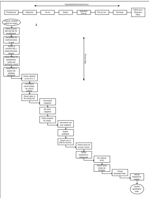
(18) therapeutic intervention are performed by physicians, nurses, and other staffs for a particular diagnosis or procedure.”. For example, Figure 2.1 shows a pathway of cholecystectomy [Guinane97]. The pathway begins with the preadmission process, which mainly involves preadmission testing and anesthesia consult, goes though a number of assessments, surgery, and physicians’ orders, and ends with a follow-up visit in the surgeon’s office.. 10.

(19) Departments/Functions/Services. Preadmission. Admission. Pre-op. Immediate Post-op. Surgery. Post-op care. Discharge. Follow-up in Physician's Office. Surgeon schedules patient for surgery Patient is given date and time for preadmission The pathway for cholecystectomy is used. Process Steps. Patient is provided with a patient-education pathway Patient arrives for preadmission testing and anesthesia consult Results sent to surgeon and admitting department. Patient admitted on the D.O..S The medical record contains the clinical pathway Patient taken to the nursing unit Assessment completed All orders completed Patient prepared for surgery Assessment and prep completed Surgery performed Patient sent to PAR for recovery Patient meets all recovery criteria Patient transferred to nursing unit. Care delivery occurs Patient meets criteria for discharge. Patient discharged home. Patient examined by surgeon. Another appointment made. Figure 2.1 A pathway of cholecystectomy. Clinical pathways, as the one shown in Figure 2.1, are driven by physician orders, and clinical industry and local standards of care. Once the pathways are created, they are viewed as algorithms in that they offer a flow chart format of the decisions to be made 11.

(20) and the care to be provided for a given patient or patient group. Therefore, clinical pathways are developed for the following purposes [Guinane97]:. -. Provide explicit and well-defined standards for care.. -. Help reduce variations in patient care (standardize care).. -. Help improve clinical outcomes.. -. Support training.. -. Provide a means of continuous quality improvement in healthcare.. -. Support clinical audit.. -. Support the use of guidelines in clinical practice.. -. Help empower patients.. -. Help manage clinical risk.. -. Help improve communications between different care sectors.. -. Disseminate accepted standards of care.. -. Provide a baseline for future initiatives.. -. Not prescriptive: don't override clinical judgment.. The application of clinical pathways is an efficient approach to analyzing and controlling clinical care processes. In today’s competitive health care environment, due to the fact that competition advantage of a healthcare institution relies not only on outstanding professional quality but also on the agile clinical care processes, the concept of clinical pathways attracts much attention of managers in large hospitals around the world [Ireson97].. From the discussion above, it can be seen that clinical pathways aim to have medical staffs doing the care services in the right order [NELH]. Take the cholecystectomy 12.

(21) pathway in Figure 2.1 as an example. Care activities are sequenced on a timeline so that physicians can make suitable orders in accordance with the test results in the preadmission step; anesthetic can be executed during the performance of surgery on the basis of anesthesia consult. Best practice, without rework and resource waste, performs if the arrangement is in the right order.. This concept of clinical pathways shows great promise on detecting service providers’ fraud and abuse. A care activity is very likely to be fraudulent if it orders suspiciously. For example, since physicians perform treatments in terms of test results, treatments following no diagnosis/test activities are doubtful; since physicians prefer performing simple, noninvasive tests before performing more complex and/or invasive tests, there is a high possibility tha t the same set of care activities performed in a different order is fraudulent or abusive.. Extensively, to accurately estimate the likelihood of a care activity performed on a particular patient, we must take into account the other activities performed on the patient. For example, while single ambulant visit is normal, repeating events are problematic, especially in the case that averaging length of pathway instances is small. On the contrary, a kidney transplant that rarely occurs should not be considered so unlikely if the patient has already undergone a series of diagnostic tests typically used to detect kidney disease.. Such observation, therefore, initiates an interesting idea that the clinical structures, including care activities and their execution orders, has the potential to discriminate. 13.

(22) between normal and fraudulent practices. Explorative analysis of our dataset 1 supports this argument. In our data set, for example, about 40% fraudulent instances contain a structure of repeating ambulant visits while only 6% normal instances do so. In this research, we are thus motivated to exploit the discriminating power of clinical structures.. Confusion often arises over the differences between clinical pathways and packages of care. Clinical pathways are elements, or chunks of care service. Each chunk of service is developed into a clinical pathway, setting out detailed processes, i.e., a collection of activities, and done as a whole [NELH]. A Package of Care may contain one or more clinical pathways selected for a particular patient or target patient group. It describes the whole range of care given to that patient or patient group, usually for one episode of care.. Many factors, such as patients’ conditions, physicians’ preferences, and management cost may influence the selection of clinical pathways in a package of care given to a particular patient. Besides, different medical institutes often enforce different pathways, as there does not yet exist a universally best practice for a disease. Therefore, each patient may have a different practice (an instance). For our purpose−exploiting the clinical structures to discriminate between normal and fraudulent instances, it is necessary to find structures from practice instances since a complete definition of care package does not exist.. Therefore, we conceive to discover structures from practices−normal and fraudulent instances. To exploit the discriminating power of the discovered structures, we adopt 1. Detailed descriptions of the data set are given in Chapter 4.4. 14.

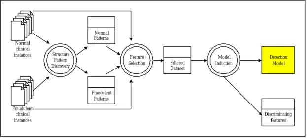
(23) an induction scheme to construct the detection model. Based on the detection model, new coming instances can be detected automatically and systematically. In this research, we explore the advantages of knowledge discovery, rather than knowledge engineering, to detect service providers’ fraud and abuse.. 2.4 Research Framework Motivated by the concept of clinical pathways, we propose a framework for detecting service providers’ fraud and abuse. Generally, as shown in Figure 2.2, two sets of clinical instances, which are labeled as normal and fraudulent, serve as the input of structure pattern discovery module. The structure pattern discovery module produces a set of frequently occurred structure patterns, which then serve as features of clinical instances. Each clinical instance is seen as an example that comprises an assignment of features and a class label (normal or fraudulent). The resultant data set is further filtered by a feature selection module to eliminate redundant and irrelevant features. The selected features and the dataset are finally used to construc t the detection model, performed by the induction module. The detection model will be used to detect the incoming instances that are fraudulent.. 15.

(24) Normal clinical instances. Normal Patterns Structure Pattern Discovery. Feature Selection. Filtered Dataset. Model Induction. Detection Model. Fraudulent Patterns Fraudulent clinical instances. Discriminating features. Figure 2.2 Research framework. In the research framework, we thereby identify three issues and form our series of investigations as below.. (1) The problem of how to discover structure patterns from clinical instances. As shown in Figure 2.1, a clinical pathway typically comprises a set of care activities. These activities, each appears over a temporally extended interval, may execute in a particular transition way, such as sequentially, concurrently, or repeatedly. A clinical instance, which consists of care activities from one or more clinical pathways, is thus formed as a set of activities in process. How to take these characters into account and design methods to efficiently discover structure patterns is the first problem we faced.. (2) The problem of how to select relevant feature s. Clearly, it is not the case that all discovered patterns have discriminating power. A certain percentage of patterns can be found in both normal and fraudulent cases and thus are irrelevant with respect to the detection problem. Also, a certain percentage of patterns are. 16.

(25) correlated and thus form redundant features. How to efficiently eliminate these redundant and irrelevant features to improve the performance of the subsequent (induction) model construction is the second problem in which we are interested.. (3) The problem of how to revise the detection model when the number of labeled examples is small. The input to the proposed research framework consists of two sets of labeled instances, those classified by experts as normal and fraudulent cases. In practice, requiring a large number of labeled training examp les to learn accurately is often prohibitive. Therefore, it is necessary to revise the existing detection model that is constructed from only labeled instances because they tend to learn less accurately for a small set of data. How to integrate other sources, such as unlabeled instances, to improve the accuracy of the detection model is another important issue in our research.. We investigate the issues listed above in order and report research results in the subsequent chapters.. 17.

(26) Chapter 3 Structure pattern discovery In order to construct the detection model described in antecedent chapter, we need to extract patterns in a way amenable to represent structures of clinical instances. In this chapter, we explore the entrance problem: the structure pattern discovery.. Typically, a clinical instance, as described in Section 2.3, is a process instance comprising a set of activities, each a logical unit of work performed by a medical staff. For example, a patient treatment flow may involve measur ing blood pressure, examining respiration, and medicine treatment, just to name a few. These activities, each appearing over a temporally extended interval, may execute sequentially, concurrently, or repeatedly. For example, before giving any therapeutic intervention, diagnosis activities are often executed to verify conditions of a patient. Also, in order to gain better curative effect in some cases, it is necessary to execute a number of therapeutic interventions concurrently.. As a result, if we want to extract structure patterns from clinical instances, we need to take structural characteristics of process−temporally extended intervals and various transition ways−into consideration. We accordingly use a temporal graph to represent a clinical instance in our research. Detailed definitions of temporal graph and corresponding algorithms for discovering patterns are described in this chapter. The experimental results in evaluating performance of the proposed algorithms are also reported.. 18.

(27) 3.1 Related works The works reported in [AGL98, Datta98, HY02] deal with the problem of discovering a process model from a set of process instances and assume the existence of a process model (i.e., control dependencies between activities) underlying a given set of process instances. In this vein, such discovery, using a directed graph [AGL98, HY02] or a finite state machine [Datta98] for representing process instances, aims at discovering a process model that best describes the set of process instances. Our study significantly differs from the process model discovery in that we do not assume the existence of an underlying process model but is designed to identify frequently observed temporal dependencies within process instances rather than control dependencies that are presumably genuine in the process instances.. Our work is closest to sequential pattern discovery that discovers frequent sequential occurrence of activities (e.g., items purchased) across transactions of the same entity (e.g., customer) [AS95, SA96]. The sequential pattern discovery is to find the maximal sequences among all sequences that have a certain user-specified minimum support. The work on sequential pattern discovery assumes that a transaction contains a set of activities occurring at the same time and that transactions of the same entity are sequentially ordered. While we assume that an activity appears over a temporally extended interval, two activities may overlap or occur in sequence, making sequential pattern discovery inappropriate because grouping activities into transactions cannot capture all possible temporal relationships between activities.. In addition, graph-based mining techniques are proposed in [CH00] that identifies interesting and repetitive substructures within structural data. Representing structural. 19.

(28) data as a labeled graph, the substructure discovery techniques aim at finding all possible substructures from the graph. By its nature, the techniques discover only substructures that are regionally connected subgraphs and disregards transitive relationships among objects, limiting its applicability to our structure pattern discovery problem, where transitivity in temporally sequential relationships prevails.. Finally, [BWJ98] deals with the discovery of frequent-event patterns in a time sequence that consists of a set of time-stamped events. The discovery process starts with a user-specified event structure that consists of a set of variables representing events and temporal constraints between variables. Its goal is to identify instantiations of variables in the event structure that appear frequently in the time sequence. The event pattern discovery differs from our work in several ways. First, it assumes an event appears at a time point rather than over a time interval. Second, it searches for instantiations of a user-specified event structure rather than discovering all possible frequent temporal relationships among events within a time sequence.. 3.2 Formalization of structure pattern discovery problem A clinical instance comprises a set of activities, each of which is an execution unit that leads to the transition of state in the instance. The execution of an activity spans a temporally extended period. Each activity may also be associated with such information as execution entit y(s) involved, execution location and execution outcome. However, since the main intent of this research is to discover frequent activities and their associated temporal dependencies, we make use only of the starting time and ending time of an activity execution. Our view on a clinical instance can be formally described as below.. 20.

(29) Definition 3.1 A clinical instance I is a set of triplets (Vi, st, et), where Vi uniquely identifies an activity, and st and et are timestamps representing the starting time and ending time of the execution of Vi in I, respectively.. Given a clinical instance, the temporal relationship between any activity pair can be classified into two types: followed and overlapped.. Definition 3.2 In a clinical instance I, an activity Vi is followed by another activity Vj if Vj starts after Vi terminates in I. Definition 3.3 In a clinical instance I, two activities, Vi and Vj, are overlapped if Vi and Vj incur overlapped execution durations in I. Definition 3.4 An activity Vi is directly followed by another activity Vj in a clinical instance I if Vi is followed by Vj in I and there does not exist a distinct activity Vk in I such that Vi is followed by Vk and Vk is followed by Vj in I.. To represent temporal relationships between activities in a clinical instance concisely, a temporal graph is defined as follows.. Definition 3.5 The pertinent temporal graph of a clinical instance I is a directed acyclic graph G = (V, E), where V is the set of activities in I, and E is a set of edges. Each edge in G is an ordered pair (Vi, Vj), where Vi, Vj ∈ V, Vi ≠ Vj, and Vi is directly followed by Vj.. Transforming a clinical instance into its corresponding temporal graph representation is straightforward. We first traverse the activities in the given clinical instance by the 21.

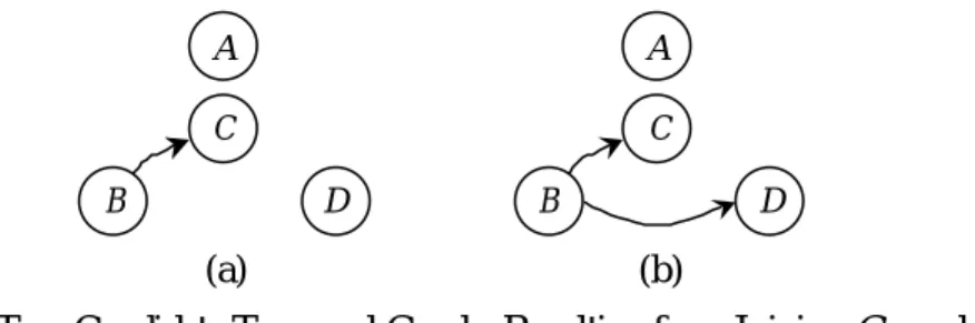
(30) ascending order of their starting times. For each activity a, the set F of activities that directly follow a are identified. Subsequently, edges connecting a to each activity in F are created. As shown in Figure 3.1(a), activity B will be processed first due to its earliest starting time among all activities in the instance. Activities C and D directly follow B; thus, two edges are created from B to C and D, respectively, as shown in Figure 3.1(b). The subsequent traversal of this clinical instance processes activities A, C, D, and E in sequence. The resulting temporal graph corresponding to this instance is graphically illustrated in Figure 3.1(b). From a given temporal graph G, it is evident that an activity Vi is followed by another activity Vj if there exists a path from Vi to Vj in G, and Vi and Vj are overlapped otherwise. As shown in Figure 3.1(b), activity B is followed by E since there exists a path from B to E. In contrast, activities A and B are overlapped since there does not exist a path that connects them.. A. A B. C. C. E D. (a) An instance. B. E. D (b) Temporal graph for the instance in (a). Figure 3.1 Example of a clinical instance and the corresponding temporal graph. A structure pattern can also be represented as a temporal graph that has a certain user-specified minimum support.. Definition 3.6 A temporal graph G is said to be supported by a clinical instance I if all followed and overlapped relationships that exist in G are present in I. Definition 3.7 A temporal graph G is said to be frequent if it is supported by no less than s% of the clinical instances, where s% is a user-defined minimum support 22.

(31) threshold. Definition 3.8 A temporal graph G=(V, E) is a temporal subgraph of another temporal graph G’=(V’, E’) if V⊆V’ and for any pair of vertices v 1 , v 2 ∈V, there is a path in G connecting v 1 to v2 if and only if there is a path in G’ connecting v 1 to v 2 . If G is a temporal subgraph of G’, then G’ is a temporal supergraph of G.. Problem statement: Given a set of temporal graphs, each of which represents a clinical instance, the structure pattern discovery is to find all frequent temporal graphs. Each such temporal graph is referred to as a structure pattern.. 3.3 Structure pattern discovery algorithms In this section, three different algorithms, namely TP-Graph, TP-Itemset, and TP-Sequence, are proposed for the described structure pattern discovery problem. TP-Graph directs its discovery process directly based on the temporal graph representation. On the other hand, TP-Itemset extends the Apriori algorithm that finds frequent itemsets [AS94] discovers patterns from a set of clinical instances, each of which is represented as a set of temporal relationships. Finally, in the TP-Sequence algorithm, each clinical instance is represented as a quasi-sequence where the overlapping and followed-by relationships of clinical instances are properly preserved. Accordingly, a sequential pattern discovery technique, specifically the AprioriAll algorithm [AS95], is extended to discover patterns from the set of quasi-sequences.. 3.3.1 TP-Graph algorithm As with association rule [AS94] and sequential pattern [AS95] algorithms, the TP-Graph algorithm exploits the downward closure property of the support measure. 23.

(32) to improve the efficiency of searching for frequent temporal graphs. The downward closure property suggests that if a temporal graph G has support of at least s%, any temporal subgraph of G must have a support of at least s% or, conversely, if a temporal graph G has a support of less than s%, any temporal supergraph of G definitely will have support of less than s%. Accordingly, we adopted an iterative procedure similar to that in the Apriori [AS94] and AprioriAll [AS95] algorithms. Specifically, potentially frequent temporal graphs (or called candidate temporal graph) of size k can be constructed from joining frequent temporal graphs of size k−1. The clinical instances are then scanned to identify frequent temporal graphs of size k from the set of candidate temporal graphs of the same size. This procedure is iteratively executed until no further frequent temporal graphs can be found. Let Ck and Lk denote the set of candidate temporal graphs and the set of frequent temporal graphs of size k, respectively. Each iteration k performs the following two steps whose challenges and solutions are detailed in the following subsections, respectively. 1.. If k=1, Ck is the set of all single-activity temporal graphs. Otherwise, join in pair-wise the frequent temporal graphs of size k−1.. 2.. Scan the clinical instances to determine Lk from Ck.. Joining frequent temporal graphs Intuitively, two frequent temporal graphs of size k−1 can be joined if they differ only in one activity and contain the same temporal relationships for any pair of common activities. However, this simple- minded joining process will result in many redundant candidate temporal graphs. Consider the following example. Suppose the set of frequent temporal graphs in iteration 2 be {A→B2 , B→C, A→C}. Any pair in the set. 2. This simplified representation differs from the temporal graph representation defined in Definition 3.5. Here, A→B denotes a temporal graph consisting of activities A and B where A is directed followed 24.

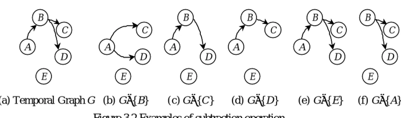
(33) can be joined to form the candidate temporal graph of A→B→C. That is, three identical candidate temporal graphs of size 3 will be generated. In the following, a joining algorithm is proposed to eliminate or control such redundancy.. Definition 3.9 Let G be a temporal graph and v be a vertex in G. The operation of substracting v from G, denoted as G−{v}, deletes v and its associated edges from G. In addition, transitive edges via v are reconstructed by connecting each source vertex of incoming edges of v to each destination vertex of outgoing edges of v.. This subtraction operation can be illustrated as follows. Figure 3.2(b)-(f) show all of the temporal subgraphs resulted from subtracting a vertex from the temporal graph G shown in Figure 3.2(a). When the vertex B is subtracted from G, edges A→C and A→D are reconstructed as shown in Figure 3.2(b). As shown in Figure 3.2(c), the deletion of the vertex C from Figure 3.2(a) does not introduce any new edge in G since C does not have any outgoing edge. Figure 3.2(d), (e), and (f) illustrate the remaining temporal subgraphs derived from Figure 3.2(a) by deleting D, E, and A, respectively.. B A. C D. E. B. C A. D E. (a) Temporal Graph G (b) G−{B}. A. B. D. B. C. A. A. E. E. (c) G−{C}. (d) G−{D}. C. B. D. D E. (e) G−{E}. (f) G−{A}. Figure 3.2 Examples of subtraction operation. Observation 3.1 Let s be a vertex without incoming edges (called a source vertex) by B. 25. C.

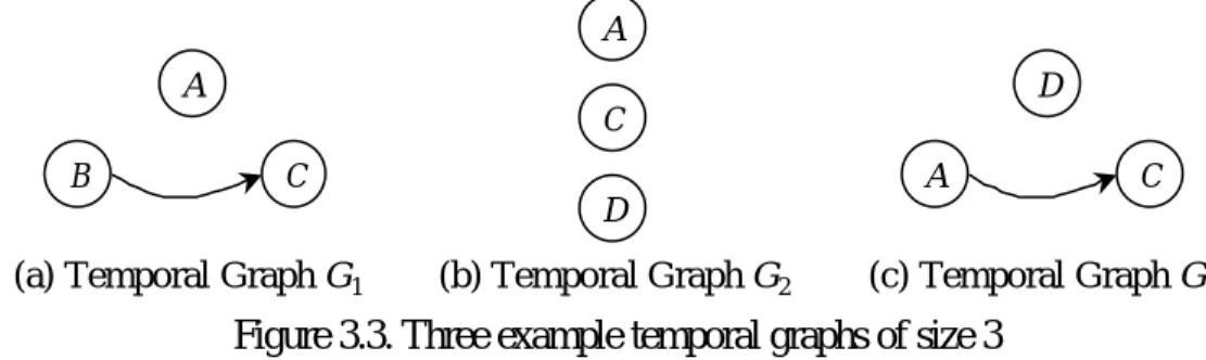
(34) and e be another vertex without outgoing edges (called a sink vertex) in a temporal graph G. If G is frequent, both G−{s} and G−{e} must be frequent.. Based on this observation, to determine whether two frequent temporal graphs can be joined, only their source vertices and sink vertices need to be considered. Accordingly, we formally define joinable temporal graphs as follows.. Definition 3.10 Two temporal graphs Gi and Gj are said to be joinable, if there exists a source vertex s in Gi and a sink vertex e in Gj such that Gi−{s} = Gj−{e}.. Consider the temporal graphs shown in Figure 3.3. Designating vertex B as a source activity of G1 shown in Figure 3.3(a) and vertex D as a sink activity of G2 shown in Figure 3.3(b), these two temporal graphs are joinable since G1 −{B} = G2 −{D}. The temporal graphs G1 and G3 or G2 and G3 , however, are not joinable.. A A B. D. C C. (a) Temporal Graph G1. D. (b) Temporal Graph G2. A. C. (c) Temporal Graph G 3. Figure 3.3. Three example temporal graphs of size 3. Given two joinable temporal graphs Gi (with s being a source vertex) and Gj (with e being a sink vertex), the temporal relationship between any pair of activities (except that between s and e) present in Gi or Gj will be preserved in a resulting candidate temporal graph. Since more than one permissible temporal relationship between s and e may exist, the joining of two joinable temporal graphs of size k–1 can lead to. 26.

(35) multiple candidate temporal graphs of size k. The temporal relationship between s and e in a candidate temporal graph can be: 1) no edge exists between s and e or 2) an edge connects s to e. Note that the case where an edge connects e to s needs not be considered, as it results in a temporal graph with s and e not being source and sink vertices respectively. From Observation 3.1, it is clear that if a temporal graph G with a source vertex s and a sink vertex e is frequent, both frequent temporal graphs G−{s} (where s is a source vertex in G) and G−{e} (where e is a sink vertex in G) must be joinable. Formally, the join set of two joinable temporal graphs Gi (with s being the source vertex) and Gj (with e being the sink vertex) is composed of 1.. Gi ∪ Gj3 , and. 2.. Gi ∪ Gj ∪ {s→e} if there does not exist a path from s to e in Gi ∪ Gj.. Consider the two joinable temporal graphs G1 and G2 shown in Figure 3.3. The join set of G1 (with B being a source vertex) and G2 (with D being a sink vertex) includes two candidate temporal graphs of size 4 as shown in Figure 3.4.. A. A. C. C. B. D. B. (a). D. (b). Figure 3.4 Two Candidate Temporal Graphs Resulting from Joining G1 and G2 in Figure 3.3. The described downward closure property can further be exploited to reduce the set of resulting candidate temporal graphs. A candidate temporal graph G of size k will not be frequent if any of its temporal subgraphs of size k−1 is not in Lk-1 and, hence, 3. The union of two graphs Gi =(Vi , Ei ) and Gj =(Vj , Ej ) results in a new graph G=(Vi ∪Vj , Ei ∪Ej ). 27.

(36) should be eliminated from Ck. Such pruning process requires, for each candidate temporal graph of size k, the derivation (using the subtraction operation defined in Definition 3.9) of all of its temporal subgraphs of size k–1. The pseudo code of GenerateCandidateGraph() for generating a set of candidate temporal graphs of size k from a set of frequent temporal graphs of size k−1 and that of DeriveSubgraph() for deriving all temporal subgraphs of size |G|−1 for a temporal graph G are listed below.. GenerateCandidateGraph(a set of frequent temporal graphs: TGS): a set of temporal graphs { CandidateSet = Ø; For (each pair of graphs (Gi, Gj) in TGS) { For (each source vertex s in Gi) { For (each sink vertex e in Gj) { If (Gi−{s}= Gj−{e}) { /* joinable */ UG1 = Gi ∪ Gj; UG2 = Gi ∪ Gj ∪ {s→ e}; CandidateSet = CandidateSet ∪ {UG1}; If there exists no path from s to e in UG1 Then CandidateSet = CandidateSet ∪ {UG2}; } /* end-if */ } /* end-for*/ } /* end-for */ } /* end-for*/ For (each graph G in CandidateSet) { If DeriveSubgraph(G) ∩ TGS ≠ DeriveSubgraph(G) Then CandidateSet = CandidateSet – {G}; } /* end-for */ Return CandidateSet; }. DeriveSubgraph(a temporal graph: G): a set of temporal graphs { Subgraph = Ø; For (each vertex v in G) { Source = the set of vertices incident to v; Sink = the set of vertices incident from v; SG = G – {v}; For (each vertex pair (v s, v d ) where v s ∈ Source and v d ∈ Sink) { If there does not exist a path between v s and v d in SG then SG = SG ∪{v s→ v d }; } /* end-for */ Subgraph = Subgraph ∪ {SG}; 28.

(37) } Return Subgraph; }. Scanning clinical instances To find frequent temporal graphs from a set of candidate temporal graphs, we have to compute their support by scanning the set of clinical instances. To efficiently decide the set of candidate temporal graphs that a given clinical instance supports, we adopted the hash-tree data structure proposed by Agrawal and Srikant [AS94, AS95]. Use of the hash-tree to store candidate temporal graphs of the same size requires a total order on the vertices in each temporal graph. In this study, the vertices of each temporal graph are sorted based on its graph topology. A topological sort of graph G is a linear ordering of all its vertices such that if G contains an edge (u, v), then u appears before v in the ordering [CLR89]. To ensure a unique topological sort for a given temporal graph, the lexicographic order is applied to vertices that are temporally overlapped. The resulting order is called the temporal sequence of a temporal graph. For instance, the temporal sequence of the temporal graph shown in Figure 3.4(a) is <B, A, C, D>.. A node in the hash-tree either contains a set of temporal graphs (a leaf node) or a hash table (an interior node). Each bucket in the hash table of an interior node points to a child node. To insert a candidate temporal graph G, we start from the root and follow appropriate pointers until a leaf node is reached. At an interior node at depth d (assuming the depth of the root node of the hash-tree be 1 and that of a child node of an interior node at depth d be d+1), we decide which branch to follow by applying a hash function to the d-th vertex in the temporal sequence of G. Initially, the root node is a leaf node. When a leaf node L at depth d overflows (i.e., the number of temporal 29.

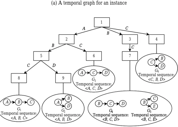
(38) graphs in the leaf node exceeds a specified threshold), L is converted to an interior node and several leaf nodes are created as the child nodes of L. All the temporal graphs originally stored in L are distributed to these leaf nodes by applying the hashing function to the d-th vertices in their temporal sequences.. Such a hash-tree, once constructed, can be used to determine the subset of candidate temporal graphs that is supported by a given clinical instance I by traversing the hash-tree. Let S denote the temporal sequence of I. The traversal starts at the root node by applying the hashing function on every vertex in S to determine the set of nodes at depth 2 to visit. At an interior node to which a vertex a in S has just hashed, the hashing function is then applied to each vertex after a in S. The traversal process continues until leaf nodes are reached. At each leaf node reached, we determine which of the candidate temporal graphs in the leaf are supported by I and increment their support count by one. After scanning all the clinical instances, the candidate temporal graphs whose support exceeds the user specified minimum threshold form the set of frequent temporal graphs of this iteration.. Consider a segment of hash-tree for candidate temporal graphs of size 3 as shown in Figure 3.5. By hashing on every vertex in the temporal sequence <B, C, E, D> of the clinical instance I shown in Figure 3.5(a), we examine those nodes that start with B, C, E, or D, respectively. In this case, the nodes 3 and 4 will be visited next. At node 3 in the hash-tree shown in Figure 3.5(b), we can only hash on vertex C, E and D since we have reached node 3 by previously hashing on vertex B. As a result, node 7 will then be visited. On the other hand, since node 4 is a leaf node, whether its candidate temporal graph (i.e., G6 ) is supported by I is then examined. Similarly, the temporal graphs (i.e., G4 and G5 ) in node 7 will be examined aga inst I and the support of G4 is 30.

(39) incremented by one since it is supported by I.. B. C. E. D. (a) A temporal graph for an instance. 1 A. C. B. 2. 3. B. C. C. 5 C. 6. B. D A. 9. C. G1 Temporal sequence: <A, B, C>. 7 C. 8. A. 4. A. C. D G6 Temporal sequence: <C, B, D>. D. G3 Temporal sequence: <A, C, D> B. B. D G2 Temporal sequence: <A, B, D>. C. B. D. B. C. E G4 G5 Temporal sequence: Temporal sequence: <B, C, D> <B, C, E>. (b) A Segment of Hash-tree. Figure 3.5 Hash-tree for candidate temporal graphs of size 3. The pseudo code for inserting a candidate temporal graph into a hash-tree, named AddOneGraph(), and that for traversing the hash-tree for a given clinical instance, named Traverse(), are listed below. Note that Traverse() is a recursive function that takes three parameters, namely the current node C of the hash-tree, the target clinical instance I, and the position of the vertex in I that previously hashed to C. Initially, we call Traverse(root of the hash-tree, I, 0).. 31.

(40) AddOneGraph(a hash-tree: T, a temporal graph: G with temporal sequence <v 1 , v 2 , …, v n >) { C = root of T; Level = 1; /* initialize */ While C is not a leaf node of T do { C= Hash(v Level ); Level++; } Insert G into C; If C is full { Create a hash table H with each entry pointing to a new leaf node; For each temporal graph R in C { Assign R to a leaf node by hashing on its vertex at depth Level; } /* end-for */ Assign the hash table H to C; } /* end-if */ } Traverse(a node pointer: C, a clinical instance: I with temporal sequence <v 1 , v 2 , …, v n >, previous position: s) { If (C is a leaf node) { For (each temporal graph G in C) { If G is supported by I then G.count++; } /* end-for */ } else { position = s; Do { NewC = Hash(v position ); Traverse(NewC, I, position+1); position++; } While (position ≤ n); } /* end-if */ }. Theorem 3.1 shows that this traversal procedure indeed returns the desired result. Lemma 3.1 For each candidate temporal graph G supported by a clinical instance I, the temporal sequence of G must be a subsequence4 of the temporal sequence of I.. 4. A sequence X = <x1 , x2 , …, xm > is a subsequence of another sequence Y = <y1 , y2 , …, yn > if there exists a strictly increasing sequence <i1 , i2 , …, im > of indices of Y such that for all j = 1, 2, …, m, we 32.

(41) Proof: Let SG = <v 1 , v2 , …, v n > and SI be the temporal sequences of G and I, respectively. For any pair of vertices v i and v j in SG where i < j, there are two possibilities on their temporal relationships: v i is followed by v j in G, and v i and v j are overlapped but v i precedes v j lexicographically. Since I supports G, it is clear that in either case the same relationship holds between v i and v j in I. Therefore, v i appears before v j in SI.. Theorem 3.1 For a given clinical instance I, the traversal of the hash-tree examines every candidate temporal graph supported by I. Proof: It is obvious that the traversal of the hash-tree for I visits the nodes by exhausting all the subsequences of the temporal sequence of I. According to Lemma 1, these nodes include all the candidate temporal graphs supported by I.. Use of a hash-tree at iteration k cannot only facilitate fast counting the support of candidate temporal graphs of size k but also improve efficiency of constructing the set of candidate temporal graphs of size k+1. Considering the hash-tree for candidate temporal graphs of size 3 shown in Figure 3.5, suppose that the temporal graph G1 (i.e., A→B→C) has been found to be frequent. To find temporal graphs that are joinable with G1 , we need only to visit those leaf nodes that are reachable by hashing on B followed by C (assuming A is selected as the source vertex in G1 ). In this case, both temporal graphs contained in the node 7 (i.e., G4 and G5 ) are joinable with G1 . This search process, of which correctness is ensured by Theorem 3.2, greatly reduces the overhead required to establish joinable temporal graphs for a given temporal graph.. have xj = yi j [CLR89]. 33.

(42) Theorem 3.2 Let G be a frequent temporal graph with the temporal sequence being <v1 , v2 , …, v n >. There must exist two joinable frequent temporal subgraphs G1 and G2 with temporal sequences being <v 1 , v 2 , …, v n-1 > and <v 2 , v3 , …, v n > respectively. In addition, the join set of G1 and G2 includes G. Proof: It is obvious from Observation 3.1 that subtracting v n from G results in a frequent temporal subgraph G1 with the temporal sequence being <v 1 , v2 , …, v n-1 > and that subtracting v 1 from G results in a frequent temporal subgraph G2 with a temporal sequence equal to <v 2 , v3 , …, v n >. Besides, since G2 −{v n } = G1 −{v1 }, G1 and G2 are joinable, and their join set includes G.. 3.3.2 TP-Itemset algorithm TP-Itemset extends the Apriori algorithm for discovering patterns from a set of clinical instances. In TP-Itemset, each possible temporal relationship in a clinical instance I is explicitly represented as an item in the itemset for I. Each item in an itemset is of the form v i→v j if the activity v i is followed by v j or v i~ v j if the durations of activities v i and v j are temporally overlapped (where ~ denotes an overlapping relationship and v i < v j in their lexicographical order). For example, as shown in Figure 3.6, the clinical instance 1 is represented as {A~B, A→C, B→C}, while the clinical instance 2 is represented as {A~B, A→C, B~C}. With this representation, n(n-1)/2 items are required to represent a clinical instance possessing n activities.. A B. A C. C B. (a) Instance 1. (b) Instance 2. Figure 3.6 Examples of two clinical instances 34.

(43) As with the association rule discovery technique, an itemset that has certain user-specified minimum support is called a large itemset, while a potentially large itemset is called a candidate itemset. The TP-Itemset algorithm is similar to the Apriori algorithm but with one distinction. Unlike in the Apriori algorithm, where resulting large itemsets are unrestricted, a large itemset generated by the TP-Itemset algorithm needs to satisfy additional constraints. Let VS = {v 1 , v 2 , … , v k} be the set of distinct activities involved in an itemset S. An itemset S is referred to as a full itemset if the temporal relationship between any pair of activities, v i and v j where v i ∈ VS , v j ∈ VS , and v i ≠ v j, exists in S. Otherwise, S is a partial itemset due to the absence of some temporal relationships in S. In effect, each full and large itemset corresponds with a frequent temporal graph defined in Definition 3.7. For instance, {A~B, A→C, B→C} is a full itemset, while {A~B, A→C} is a partial itemset because the relationship between activities B and C is unspecified. Hence, large itemsets generated by the TP-Itemset algorithm are required to be full itemsets.. Given a set of clinical instances, the TP-Itemset algorithm transforms them into a set of full itemsets and generates the itemsets among all full and large itemsets. Each such full and large itemset represents a structure pattern. Let Lk be a set of large k-itemsets each of which has k items (i.e., k temporal relationships) and Ck be a set of candidate k-itemsets, where Ck can be constructed by joining large itemsets in Lk–1 . In the Apriori algorithm, the joining procedure requires that items within an itemset be kept in their lexicographic order. In this study, since each item (v i→v j or v i~ v j) involves two activities, the lexicographical order of a set of items is based on their first activities (i.e., v i) and then on their second ones (i.e., v j). Moreover, the partial itemsets from Lk–1 should not be removed immediately at each iteration k–1, since two 35.

(44) partial (k–1)-itemsets may result in a full itemset in Ck. For instance, joining two partial, large itemsets in L2 , {A→B, A→C} and {A→C, B~C}, results in a full itemset {A→B, A→C, B~C}. Finally, to facilitate fast counting the support for the candidate itemsets in Ck, candidate itemsets are stored in a hash-tree as employed by the Apriori algorithm [AS94]. Accordingly, the TP-Itemset algorithm for discovering structure patterns is listed below.. TP-Itemset(a set of process instances: I, the minimum support: minsup): a set of large and full itemsets { Transform each clinical instance i ∈ I into a itemset s in S; L1 = {large 1-itemsets}; MaxK= 1; For (k = 2; Lk-1 ≠Ø; k++) { Generates candidate itemsets Ck from Lk-1 ; For each itemset s ∈ S { Ct = subset5 (Ck, i); // find candidate itemsets that are supported by i For each candidate c ∈ Ct do c.count++; } /* end-for */ Lk = {c ∈ Ck | c.count ≥ minsup}; If (Lk ≠Ø) then MaxK = MaxK+1; } /* end-for */ For (k=MaxK; k>1; k--) { Prunes partial itemsets in Lk; } /* end-for */ Return ∪k≥1 Lk; }. 3.3.3 TP-Sequence algorithm TP-Sequence is based on the sequential pattern discovery technique (specifically, the AprioriAll algorithm) to discover patterns from a set of clinical instances. In the TP-Sequence algorithm, the overlapped and followed relationships in each clinical 5. Using the hash-tree constructed for Ck, the subset(Ck, i) function is to find all the candidate itemsets in Ck that are supported by the itemset i. We employed and implemented the subset function as proposed in [AS94]. 36.

(45) instance are explicitly represented as a sequence, where an itemset is a non-empty set of overlapping activities, and a sequence is an ordered list of itemsets. The itemset (x, y) denotes that activities x and y are temporally overlapped. A sequence with an order list of k itemsets is called a k-sequence. For instance, a 2-sequence <(x)(y)> denotes that the activity x is followed by y. Furthermore, a 2-sequence <(x, y)(y, z)> denotes that activity x is followed by z, while y overlaps with x and z. As shown in Figure 3.6, the clinical instance 1 is represented as a sequence of <(A, B) (C)>, while the clinical instance 2 is represented as <(A, B) (B, C)>. Using this representation, a clinical instance is represented as an m-sequence where l ≤ m ≤ n, l is the number of activities in the longest path in the respective temporal graph, and n is the number of activities in the clinical instance.. In the sequential pattern discovery, no specific constraint is imposed on itemsets in a sequence. However, since a sequence in the TP-Sequence algorithm is used to represent both the followed and overlapped relationships, a meaningful sequence needs to satisfy certain constraints. We call a sequence <(x) (x, y)> a non-canonical sequence since it is identical to <(x, y)>. On the other hand, <(x, y) (w) (x, z)> is an illegitimate sequence since both “x followed by w” and “w followed by x” exist; thus, violating the irreflexivity of followed relationships. Hence, for discovering structure patterns, the AprioriAll algorithm needs to be extended to ensure that any candidate sequence generated be canonical and legitimate. Let ai be an itemset. Non-cano nical and illegitimate sequences are formally defined as follows.. Definition 3.11 A sequence s = <a1 a2 … am > is canonical if for each itemset aj, 1≤ j < m, aj ⊄ aj+1 and aj+1 ⊄ aj. Definition 3.12 A sequence s = <a1 a2 … am > is legitimate if for each item x 37.

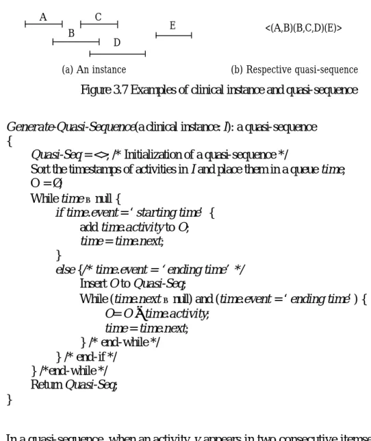
(46) involved in s, the itemsets that contain x form a continuous sequence in s.. To distinguish an unconstrained sequence from a sequence with canonicity and legitimacy properties (as required by the TP-Sequence algorithm), the latter is called a quasi-sequence. The transformation of a clinical instance I into its respective quasi-sequence proceeds in the following iterative manner. The quasi-sequence is initialized as an empty list. We traverse the starting and ending times of activities in I in ascending order. The set O of overlapped activities is accumulated each time a starting time is visited. When the first ending time is encountered, the set O is appended to the quasi-sequence. Subsequently, we continue the traversal until the next starting time (assuming its respective activity be v) is visited. The subset of activities in O whose ending times appear before the starting time of v are removed from O since this subset of activities that have appeared in the quasi-sequence are followed by v. This traversal procedure continues until all the timestamps are visited. Let us illustrate this transformation using the clinical temporal grap instance shown in Figure 3.7(a). As shown, when the first ending time (which belongs to A) is visited, O=(A, B) and, thus, the current quasi-sequence is <(A, B)>. Since there no ending times appear before the next starting time (that pertains to C), only A is removed. When the next ending time (that pertains to B) is visited, O=(B, C, D) and, therefore, the quasi-sequence becomes <(A, B) (B, C, D)>. When the following starting time (that is possessed by E) is visited, O becomes empty because the ending times of B, C, and D have all been traversed. When the last ending time (which belongs to E) is visited, O=(E), and the resultant quasi-sequence is <(A, B) (B, C, D) (E)> as shown in Figure 3.7(b). The pseudo-code of the described transformation is listed in the following.. 38.