交通大學
機械工程學系
博士論文
平行化三維
DSMC-NS 偶合數值方法之發展及驗證
Development and Verification of a Parallel Coupled DSMC-NS
Scheme Using A Three-dimensional Unstructured Grid
學生 連又永
指導教授 吳宗信 博士
平行化三維
DSMC-NS 偶合數值方法之發展及驗證
Development and Verification of a Parallel Coupled DSMC-NS SchemeUsing A Three-dimensional Unstructured Grid
研 究 生:連又永
Student:Yu-Yung Lian
指導教授:吳宗信 博士
Advisor:Dr. Jong-Shinn Wu
國 立 交 通 大 學
機 械 工 程 學 系
博 士 論 文
A ThesisSubmitted to Institute of Mechanical Engineering Collage of Engineering National Chiao Tung University
in Partial Fulfillment of the Requirements for the Degree of
Doctor of Philosophy in Mechanical Engineering July 2006 Hsinchu, Taiwan
中華民國九十五年七月
Development and Verification of a Parallel Coupled DSMC-NS Scheme
Using A Three-dimensional Unstructured Grid
Student:Yu-Yung Lian Advisors:Dr. Jong-Shinn Wu
Department of Mechanical Engineering National Chiao Tung University
Abstract
In this thesis, an efficient and accurate parallel coupled DSMC-NS method using
three-dimensional unstructured grid topology is proposed and verified for the simulation of
high-speed gas flows involving continuum and rarefied regimes. In addition, breakdown
parameters near the solid wall are reinvestigated by a detailed kinetic study and a new
criterion of breakdown parameter is proposed. Research in this thesis is divided into two
phases, which are described in the following in turn.
In the first phase, a parallel coupled DSMC-NS method using three-dimensional
unstructured grid topology is proposed and verified. A domain overlapping strategy, taking
advantage of unstructured data format, with Dirichlet-Dirichlet type boundary conditions
based on two breakdown parameters is used iteratively to determine the choice of solvers in
the spatial domain. The selected breakdown parameters for this study include: 1) a local
characteristic length based on property gradient and 2) a thermal non-equilibrium indicator
defined as the ratio of the difference between translational and rotational temperatures to the
translational temperature. A supersonic flow (M∞=4) over a quasi-2-D 25° wedge is
employed as the first step in verifying the present coupled method. The results of simulation
using the coupled method are in excellent agreement with those of the pure DSMC method,
which is taken as the benchmark solution. Effects of the size of overlapping regions and the
choice of breakdown parameters on the convergence history are discussed. Results show that
the proposed iteratively coupled method predicts the results more accurately as compared to
the “one-shot” coupled method, which has been often used in practice. Further, two realistic
3-D nitrogen flows are simulated using the developed coupled DSMC-NS scheme. The first
one is a flow, which consists of two near-continuum parallel orifice jets underexpanding into
a near-vacuum environment. The second one is a flow issuing from a typical RCS (Reaction
Control System) thruster. Results are compared with experimental data wherever is available.
In the second phase, a detailed kinetic investigation using the DSMC method is used to
re-examine previous proposed criteria of continuum breakdown parameters by studying the
supersonic flow past a finite-size wedge flow. Choice of this particular flow for kinetic study
lies in the fact that it includes a leading edge, a boundary layer, an oblique shock and an
expanding fan, which covers most critical flow phenomena for the present hybrid DSMC0-NS
are sampled and compared with the corresponding local Maxwell-Boltzmann distribution. In
addition, degree of thermal non-equilibrium among various degrees of freedoms is computed
at these locations. To efficiently indicate the degree of thermal non-equilibrium among
various degrees of freedoms, a general indicator of thermal non-equilibrium, with its
threshold value 0.03, is used with the consideration of temperature deviations among different
temperature modes, including translational temperatures in the three Cartesian directions,
rotational temperature and vibrational temperature. From the results, it is found that the
degree of the continuum breakdown in the boundary-lay region is overestimated with the
previously recommended threshold value of . max
Thr
Kn 0.05. Revised criterion near the
isothermal solid wall is proposed as 0.8 in the present study.
Key words: direct simulation Monte Carlo (DSMC), coupled method, rarefied gas flow,
平行化三維 DSMC-NS 偶合數值方法之發展及驗證
學生:連又永 指導教授:吳宗信 博士 國立交通大學機械工程學系博士班中文摘要
本論文提出一個兼顧效率及準確度的平行化三維非結構性網格之直接蒙地卡羅法 與Navier-Stokes 偶合數值方法。本文中針對幾個同時涉及連續體及稀薄流域之高速氣流 場進行模擬,以驗證該偶合數值方法之正確性。藉由使用直接蒙地卡羅法進行詳盡的分 子動力學研究重新檢視,在靠近固體邊界區連續流假設失效參數的使用,並且提出新的 連續體假設失效與否的新標準。以下,將本論文的工作分成兩個階段分別來介紹。 第一階段,本論文先提出一個平行化、使用三維非結構性網格的直接蒙地卡羅法與 Navier-Stokes 偶合數值方法。本方法是反覆地根據兩個連續體失效參數來決定在空間上 各個區域其數值方法的選擇。利用非結構性網格的優點,採用數值方法區域重疊 (Domain Overlapping)策略,流場性質在邊界上的交換則採用固定式的邊界交換形式 (Dirichlet-Dirichle type)。在本論文中所採用的兩個連續體失效參數包括: 1)區域性最大紐森數(local maximum Knudsen number),其定義為,氣體分子平均自由徑除以流體性質梯
度所定義之特徵長度,以及 2)熱力平衡指標數,其定義為: 移動動能分布溫度與旋轉動
我們針對超音速(M∞=4)氣流流過一個近似二維的 25°之楔形體作為驗證的第一個算例。 在這個驗證算例中,未經偶合的直接蒙地卡羅法視為是對照用的正確解。利用本文提出 之偶合方法跟未經偶合的直接蒙地卡羅法的比較結果極為吻合。關於數值方法重疊區域 (Overlapping Region) 的大小以及連續體失效參數標準大小的選用,對於這個偶合方法 收斂性的影響也在本論文有所討論。這個算例結果顯示,相較於實務上常被使用的一次 交換邊界的偶合 (One-shot coupled) 方法,目前本論文提出的反覆進行數值方法疊代之 偶合數值方法可以更正確地預測流場結果。更進一步,將使用本論文目前所提的偶合數 值方法,針對兩個真實三維氮氣場算例進行模擬:第一個是擴散到幾乎真空的環境的平
行雙孔噴流,第二個則是衛星姿態控制器(Reaction control system)的噴嘴形成的氣流
場,而模擬結果將與現有的實驗結果進行比較。
為了重新檢驗過去研究工作所建議的連續體失效參數的判斷標準,本論文的第二階
段將以直接蒙地卡羅法,針對超音速氣流流經一個有限長度的楔形體的算例,進行詳盡
的分子動力學研究。選用該流場作為分子動力學分析的原因是本算例的流場同時存在銳
緣區(leading edge)、邊界層區、斜震波區以及扇形擴散區(expanding fan),這些流場區域
涵蓋了對於目前直接蒙地卡羅法與 Navier-Stokes 偶合數值方法模擬所遭遇的大多數關
鍵性之流場現象。文中在流場各個不同特定位置上,針對卡氏坐標系之三個方向速度進
行採樣,並與該位置所對應的馬斯威爾-波茲曼速度分布進行分析比較。此外,亦計算
在這些位置上的各個不同溫度自由度之間熱力不平衡的程度。為了有效定義各種不同溫
動動能溫度)之間熱力不平衡的程度,本文進一步重新定義一個更具一般性的熱力平衡 指標數,並提出以0.03 為其對應之熱力平衡臨界值。據結果顯示可發現,使用過去相關 研究所建議的區域性最大紐森數 0.05 作為判定是否連續體失效標準,對於在邊界層區 域裡連續體失效程度的判斷可能會過於高估。本論文提出針對於靠近固體邊界區域,採 用與其他區域不同的區域性最大紐森數判斷標準 0.8,作為該區域是否發生連續體失效 之判定。 關鍵字: 直接蒙地卡羅法、偶合數值方法、稀薄氣流場、Navier-Stokes 數值解法、超音 速流場
誌謝
在論文付梓之際,心中滿是感謝。感謝上天的安排,讓我在交通大學度過美 好與充實的歲月,匯聚如此之因緣。 本論文得以順利之完成,首先要感謝指導教授 吳宗信教授在論文撰寫期間之 督促與悉心指導,在遭遇瓶頸時總是幫我渡過難關,解決心中的疑問。恩師在研 究工作上的積極與執著態度,是我學習的榜樣。感謝美國阿拉巴馬州大學伯明罕 分校 Gary Cheng教授促成這次出訪研究合作的機會,以及對我在美國時的種種照 顧及指導,同時也感謝伯明罕分校的Roy Koomullil教授在本研究發展初期的協 助。特別感謝國家太空中心的陳彥升博士撥冗協助學生之論文研究,並提供許多 寶貴意見,特此致上由衷謝忱。 在這段學習成長的期間,感謝所有陪伴我同甘共苦的夥伴,感謝學長 坤樟、 佑霖、雲龍及學弟妹 桂雄、允民、欣芸、捷粲,以及學弟 維呈、志偉、育進、 凱文在論文口試期間的協助。特別感謝難兄難弟國賢:我們終於畢業了!! 研究工作得以順利進行,特別感謝國家太空中心「衛星推進器引致污染及衝 擊影響分析軟體發展計畫」(93-NSPO(A)-PC-FA04-01)、美國太空總署(NASA)之 大學研究工程及技術機構計畫URETI(NCC3-994)提供相關研究論文補助。 最後,更要感謝永遠默默付出的家人之關懷與鼓勵,特別是我的父母,對我 的包容,讓我得以無憂無慮的求學。要感謝的人實在太多太多,無法一一致謝, 僅將此論文獻給我的家人、師長以及所有關心我的朋友。 連又永 謹誌于 交大風城 中華民國九十五年七月Table of Contents
Abstract ... i
中文摘要... iv
誌謝...vii
Table of Contents ...viii
List of Algorithms ... x
List of Tables ... xi
List of Figures ...xii
Nomenclature ...xvii
Chapter 1 Introduction ... 1
1.1 Background ... 1
1.1.1 Classification of Gas flows ... 4
1.1.2 Challenge to Particle-Continuum Flow Simulation ... 6
1.2 Literature Reviews ... 7
1.3 Motivation ... 9
1.3.1 Key Factors of Hybrid DSMC-NS Scheme ... 9
1.3.2 Continuum Breakdown Parameter ... 11
1.4 Objectives of the Thesis ... 12
1.5 Organization of the Thesis ... 12
Chapter 2 Numerical Methods ... 14
2.1 Direct Simulation Monte Carlo ... 14
2.1.1 General Description of DSMC... 15
2.1.2 The DSMC Procedures... 16
2.1.3 Parallel DSMC Code PDSC... 24
Variable time-step scheme... 25
2.2 Navier-Stokes Method... 26
2.2.1 General Description of Navier-Stokes Method ... 27
2.2.2 Navier-Stokes Solvers: HYB3D and UNIC-UNS Code ... 29
2.3 Hybrid DSMC-NS scheme... 31
2.3.1 Breakdown Parameters... 31
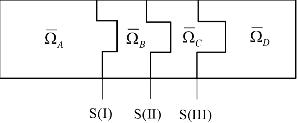
2.3.2 Overlapping Regions Between DSMC and NS Domain... 36
2.3.3 Coupling Procedures ... 39
2.3.4 Practical Implementation... 42
Chapter 3 Benchmark tests and verifications... 43
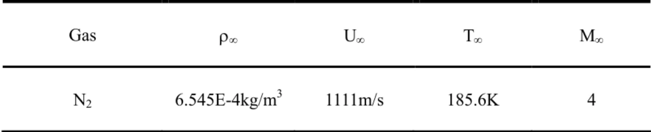
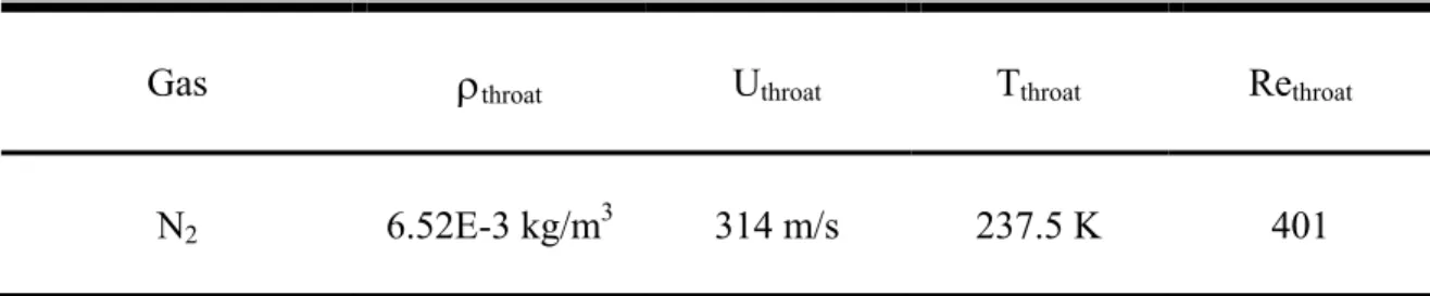
3.1 Supersonic Nitrogen Flow over a Two-Dimensional Wedge ... 43
3.1.1 Flow and Simulation Conditions... 43
3.1.3 Verification of the Coupled DSMC-NS Scheme... 50
3.1.4 Effect of the Varying Simulation Parameters on Convergence ... 53
3.2 Three-Dimensional Parallel Twin-Jets ... 54
3.2.1 Flow and Simulation Conditions... 54
3.2.2 Distributions of Flow Properties ... 55
3.2.3 Profile along Center Line between Parallel Twin-Jets ... 56
3.2.4 Convergence History of Parallel Twin-Jets... 57
3.3 Application: Plume Analysis of RCS thrusters ... 58
3.3.1 Flow and Simulation Conditions... 59
3.3.2 Properties Contour... 60
Chapter 4 Revisit to the Continuum Breakdown ... 64
4.1 Generally Thermal Non-Equilibrium Indicator... 65
4.2 Kinetic Study with a 2-D Wedge Supersonic Flow... 66
4.2.1 Flow and Simulation Conditions... 66
4.2.2 Region near the Leading Edge ... 68
4.2.3 Region near the Oblique Shock... 70
4.2.4 Region near the Boundary Layer ... 71
4.2.5 Region near the Expanding Fan ... 73
4.3 Revised Criterion of Continuum Breakdown Parameter... 74
Chapter 5 Conclusions ... 77
5.1 Summary ... 77
5.2 Recommendations for Future Work ... 79
References ... 81
Autobiography... 200
List of Algorithms
Algorithm 2.1 Procedures of locating breakdown regions and Boundary-I. ... 85
Algorithm 2.2 Procedures of locating overlapping regions and Boundary... 87
Algorithm 2.3 General procedures of the proposed coupled DSMC-NS method. ... 89
Algorithm 2.4 Procedures of extracting Boundary-III data for DSMC solver. ... 90
List of Tables
Table 3.1 Free-stream conditions in supersonic flow over quasi-2-D 25o wedge. ... 92 Table 3.2 Four simulation sets with various parameters in supersonic flow over quasi-2-D
25o wedge. ... 93 Table 3.3 Total computational time (hours) with pure NS solver, pure DSMC and coupled
method in supersonic flow over quasi-2-D 25o wedge... 94 Table 3.4 Sonic conditions at the orifice exiting plane in two parallel near-continuum orifice
free jets flow. ... 95 Table 3.5 Simulational conditions of two parallel near-continuum orifice free jets flow... 96 Table 3.6 Total computational time (hours) with pure NS solver and coupled method in two
parallel near-continuum orifice free jets flow. ... 97 Table 3.7 Flow conditions of the plume simulation issuing from RCS thruster ... 98 Table 3.8 Simulation conditions of the plume simulation issuing from RCS thruster... 99
List of Figures
Fig. 1.1 Sketch of expanding reaction control system plumes. ... 100
Fig. 1.2 Sketch of expanding flying object plume at high altitude... 101
Fig. 1.3 Sketch of a sketch of spiral-grooved turbo booster pump... 102
Fig. 1.4 Configuration of a jet-type CVD reactor... 103
Fig. 1.5 Schematic sketch of solution method applicability in a dilute gas. ... 104
Fig. 2.1 Flow chart of the DSMC method. ... 105
Fig. 2.2 Sketch of the particle movement in three-dimensional unstructured mesh. ... 106
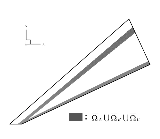
Fig. 2.3 Sketch of domain distribution of the present coupled DSMC-NS method with overlapping regions and boundaries... 107
Fig. 2.4 A typical example of the overlapping regions between the particle and the continuum domains. ... 108
Fig. 3.1 Sketch of a hypersonic flow over 25o 2-D wedge... 109
Fig. 3.2a Grid sensitivity test of HYB3D on quasi-2-D 25o wedge flow (Density)... 110
Fig. 3.2b Grid sensitivity test of HYB3D on quasi-2-D 25o wedge flow (Total temperature). ... 111
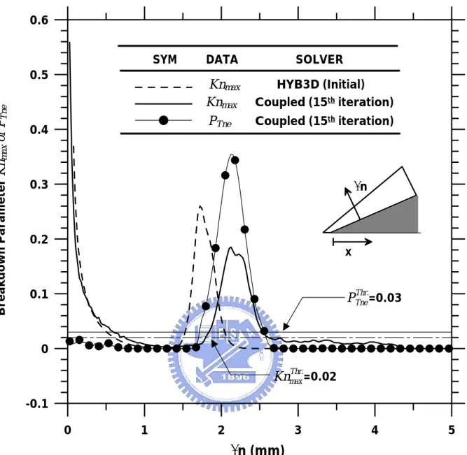
Fig. 3.3c Breakdown parameters along the line normal to the wedge at x=50mm. ... 114
Fig. 3.4a Initial continuum breakdown (NS) domain distribution in quasi-2-D 25o wedge flow... 115
Fig. 3.4b Initial DSMC domain including the overlapping regions in quasi-2-D 25o wedge flow... 116
Fig. 3.5a Breakdown domain distribution at 15th coupling iteration in quasi-2-D 25o wedge flow... 117
Fig. 3.5a DSMC domain including the overlapping regions at 15th coupling iteration in quasi-2-D 25o wedge flow. ... 118
Fig. 3.6a Density comparison between the DSMC method and the present coupled DSMC-NS method in quasi-2-D 25o wedge flow. ... 119
Fig. 3.6b Translation temperature comparison between the DSMC method and the present coupled DSMC-NS method in quasi-2-D 25o wedge flow. ... 120
Fig. 3.7a Density profile along a line normal to the wedge at x=0.5mm. ... 121
Fig. 3.7b Translational temperature profile along a line normal to the wedge at x=0.5mm. ... 122
Fig. 3.8a Density profile along a line normal to the wedge at x=5mm. ... 124 Fig. 3.8b Translational temperature profile along a line normal to the wedge at x=5mm. . 125 Fig. 3.8c Velocity profile along a line normal to the wedge at x=5mm. ... 126 Fig. 3.9a Density profile along a line normal to the wedge at x=50mm. ... 127 Fig. 3.9b Translational temperature profile along a line normal to the wedge at x=50mm. 128 Fig. 3.9c Velocity profile along a line normal to the wedge at x=50mm. ... 129 Fig. 3.10 Convergence history of L2-norm deviation of density among the four simulation
sets in quasi-2-D 25o wedge flow... 130 Fig. 3.11 Convergence history of L2-norm deviation of total temperature among the four
simulation sets in quasi-2-D 25o wedge flow. ... 131 Fig. 3.12a Comparison of density along a line normal to the wedge at x=0.5mm among the
four simulation sets. ... 132 Fig. 3.12b Comparison of translational temperature along a line normal to the wedge at
x=0.5mm among the four simulation sets. ... 133 Fig. 3.13 Sketch of two parallel near-continuum orifice free jets flow. ... 134 Fig. 3.14 Mesh distribution of two parallel near-continuum orifice free jets flow simulation.
... 135 Fig. 3.15 Surface mesh distribution of breakdown domain (DSMC domain) of two parallel
near-continuum orifice free jets flow simulation with an exploded view (after 2 coupled iterations). ... 136 Fig. 3.16 Density contours of two parallel near-continuum orifice free jets flow... 137 Fig. 3.17a Thermal non-equilibrium contours of two parallel near-continuum orifice free jets
flow... 138 Fig. 3.17b Thermal non-equilibrium contours near the orifice. ... 139 Fig. 3.18a Normalized density distribution along the symmetric line of two parallel
near-continuum orifice free jets flow. ... 140 Fig. 3.18b Density distribution along the symmetric line of two parallel near-continuum
orifice free jets flow... 141 Fig. 3.19 Rotational temperature distribution along the symmetric line of two parallel
near-continuum orifice free jets flow. ... 142 Fig. 3.20 Convergence history of density for two parallel near-continuum orifice free jets
flow... 143 Fig. 3.21 Convergence history of total temperature for two parallel near-continuum orifice
Fig. 3.22a Mach number distribution of quasi-2-D supersonic wedge flow (gray areas: DSMC
domain; others: NS domain). ... 145
Fig. 3.22b Mach number distribution of two parallel near-continuum free jets near orifice (white region: breakdown interface). ... 146
Fig. 3.23 Sketch of the plume simulation issuing from RCS thruster. ... 147
Fig. 3.24 Mesh distribution of the plume simulation issuing from RCS thruster... 148
Fig. 3.25 Spatial computational domain distributions... 149
Fig. 3.26 Domain decomposition for 6 processors (a) NS CPU domain; (b) Initial DSMC CPU domain; (c) Final DSMC CPU domain (6th iteration). ... 150
Fig. 3.27 Continuum breakdown distribution of the plume simulation issuing from RCS thruster... 151
Fig. 3.28 Distribution of non-equilibrium ratio in the RCS plume simulation. ... 152
Fig. 3.29 Particle per cell in the RCS plume simulation. ... 153
Fig. 3.30 Density distribution of the plume simulation issuing from RCS thruster (a) One-shot NS method; (b) Coupled DSMC-NS method (6th iteration)... 154
Fig. 3.31 Temperature distribution of the plume simulation issuing from RCS thruster (a) One-shot NS method; (b) Coupled DSMC-NS method (6th iteration)... 155
Fig. 3.32 Stream lines of the plume simulation issuing from RCS thruster (a) One-shot NS method; (b) Coupled DSMC-NS method (6th iteration)... 156
Fig. 3.33 Mach number distribution of the plume simulation issuing from RCS thruster (a) One-shot NS method; (b) Coupled DSMC-NS method (6th iteration)... 157
Fig. 3.34 Convergence history of density for the plume simulation issuing from RCS thruster. ... 158
Fig. 3.35 Convergence history of total temperature for the plume simulation issuing from RCS thruster. ... 159
Fig. 4.1 Surface mesh distribution of 2-D wedge flow for the kinetic study of velocity sampling. ... 160
Fig. 4.2 Locations of velocity sampling and continuum breakdown distribution of 2-D wedge flow for the kinetic study of velocity sampling. ... 161
Fig. 4.3 Domain distribution of dominating breakdown parameter of 2-D wedge flow for the kinetic study of velocity sampling... 162
Fig. 4.4a Locations of velocity sampling Point 3-7 (Leading edge region)... 163
Fig. 4.4b Random velocity distributions to each direction at Point 3 (Leading edge region). ... 164 Fig. 4.4c Random velocity distributions to each direction at Point 4 (Leading edge region).
... 165 Fig. 4.4d Random velocity distributions to each direction at Point 5 (Leading edge region).
... 166 Fig. 4.4e Random velocity distributions to each direction at Point 6 (Leading edge region).
... 167 Fig. 4.4f Random velocity distributions to each direction at Point 7 (Leading edge region).
... 168 Fig. 4.5a Locations of velocity sampling Point 14-19 (Oblique shock region). ... 169 Fig. 4.5b Random velocity distributions to each direction at Point 14 (Oblique shock region).
... 170 Fig. 4.5c Random velocity distributions to each direction at Point 15 (Oblique shock region).
... 171 Fig. 4.5d Random velocity distributions to each direction at Point 16 (Oblique shock region).
... 172 Fig. 4.5e Random velocity distributions to each direction at Point 17 (Oblique shock region).
... 173 Fig. 4.5f Random velocity distributions to each direction at Point 18 (Oblique shock region).
... 174 Fig. 4.5g Random velocity distributions to each direction at Point 19 (Oblique shock region).
... 175 Fig. 4.6b Locations of velocity sampling Point 26-30 (Boundary layer region)... 176 Fig. 4.6b Random velocity distributions to each direction at Point 26 (Boundary layer
region). ... 177 Fig. 4.6c Random velocity distributions to each direction at Point 27 (Boundary layer
region). ... 178 Fig. 4.6d Random velocity distributions to each direction at Point 28 (Boundary layer
region). ... 179 Fig. 4.6e Random velocity distributions to each direction at Point 29 (Boundary layer
region). ... 180 Fig. 4.6f Random velocity distributions to each direction at Point 30 (Boundary layer
region). ... 181 Fig. 4.7a Locations of velocity sampling Point 31-35 (Boundary layer region)... 182 Fig. 4.7b Random velocity distributions to each direction at Point 31 (Boundary layer
region). ... 183 Fig. 4.7c Random velocity distributions to each direction at Point 32 (Boundary layer
region). ... 184 Fig. 4.7d Random velocity distributions to each direction at Point 33 (Boundary layer
region). ... 185 Fig. 4.7e Random velocity distributions to each direction at Point 34 (Boundary layer
region). ... 186 Fig. 4.7f Random velocity distributions to each direction at Point 35 (Boundary layer
region). ... 187 Fig. 4.8a Locations of velocity sampling Point 41-16 (Expanding fan region). ... 188 Fig. 4.8b Random velocity distributions to each direction at Point 41 (Expanding fan region).
... 189 Fig. 4.8c Random velocity distributions to each direction at Point 42 (Expanding fan region).
... 190 Fig. 4.8d Random velocity distributions to each direction at Point 43 (Expanding fan region).
... 191 Fig. 4.8e Random velocity distributions to each direction at Point 44 (Expanding fan region).
... 192 Fig. 4.8f Random velocity distributions to each direction at Point 45 (Expanding fan region).
... 193 Fig. 4.8g Random velocity distributions to each direction at Point 46 (Expanding fan region).
... 194 Fig. 4.9 L2 norm deviation of random velocity and thermal non-equilibrium indicator as
functions of continuum breakdown parameter near the leading edge region. ... 195 Fig. 4.10 L2 norm deviation of random velocity and thermal non-equilibrium indicator as
functions of continuum breakdown parameter near the oblique shock region. ... 196 Fig. 4.11 L2 norm deviation of random velocity and thermal non-equilibrium indicator as
functions of continuum breakdown parameter near the expanding fan region. ... 197 Fig. 4.12 L2 norm deviation of random velocity and thermal non-equilibrium indicator as
functions of continuum breakdown parameter near the boundary layer region... 198 Fig. 4.13 Thermal non-equilibrium indicator as functions of continuum breakdown
Nomenclature
λ :mean free pathρ :density
σ :the differential cross section ω :viscosity temperature exponent Ω : space domain rot ε :rotational energy v ε :vibrational energy rot
ζ :rotational degree of freedom
v
ζ :vibrational degree of freedom Ut :time-step
σT :the total cross section
c :the total velocity c’ :random velocity co :mean velocity
cr :relative speed
d :molecular diameter
D :the throat diameter of the twin-jet interaction dref :reference diameter
E :energy
k :the Boltzmann constant Kn :Knudsen number
Knmax : continuum breakdown parameter
. max
Thr
Kn : the threshold value of continuum breakdown parameter Q
Kn : local Knudsen numbers based on flow property Q
L :characteristic length; m :molecule mass
M∞ :free-stream mach number
Tne
P : thermal non-equilibrium indicator .
Thr Tne
P : the threshold value of thermal non-equilibrium indicator
Re :Reynolds number To :stagnation temperature
T∞ :free-stream temperature
Tref :reference temperature
Trot :rotational temperature
Ttot :total temperature
Ttr :translational temperature
Tv :vibrational temperature
Chapter 1
Introduction
1.1 Background
Fluid dynamics is one of fields in which computer simulation shows a great deal of
promise, and interest in the development of better algorithms is strong. In a broad sense,
there are two methods by which fluid flows are simulated: continuum methods and particle
method. The former relies on the numerical solution of a set of partial differential equations,
for example Navier-Stokes equations, describing the fluid flow, with proper boundary
conditions applied. On the other hand, particle method is the other way to attempts to model
a fluid flow by simulating the interactions of particles themselves and the interactions
between particles and body boundaries. Despite of its requirement of tremendous
computational effort, particle-based method can handle gas flows involving rarefaction and
non-equilibrium phenomena, while the generally more efficient continuum method like
Navier-Stokes solver becomes invalid. The understanding of rarefied gas dynamics
(high-Knudsen number flows) plays an important role in several research disciplines, e.g.
space flight research and semiconductor processing, and many related important flow
problems of interest often are involving both of continuum and rarefied regions.
flow fields. Examples include, but are not limited to, expanding reaction control system
plumes [Taniguchi et al., 2004 and Ivanov et al., 2004], expanding plumes from a flying
projectile at high altitude [Wilmoth et al., 2004], spiral-grooved turbo booster pump with high
compression ratio [Cheng et al., 1999] and jet-type (Chemical Vapor Deposition) [Versteeg et
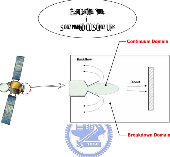
al., 1994] and will be introduced in the following. Fig. 1.1 is the sketch of expanding
reaction control system plumes. When spacecraft or satellite flies through an altitude of near
vacuum environment, the RCS thrusts are used to provide the power and control the
spacecraft or satellite. In this flow field, the flow is continuum flow from the throat and
becomes transition flow and rarefied as the flow pass through the nozzle to the space.
Usually, the thrusters are made up by a lot of small nozzles. Exhaust jets issuing from
thrusts of spacecraft produce a huge jet plume. Various jet plumes cause many types of
plume impingement on the associated or neighboring surfaces. When any part of surface
suffers impingement of the plume, undesirable effects such as contamination, heating,
disturbance torque and erosion will damage to the safety of spacemen and cause an
anomalous behavior of the instruments. Thus, simulation of the plume impingement is very
important.
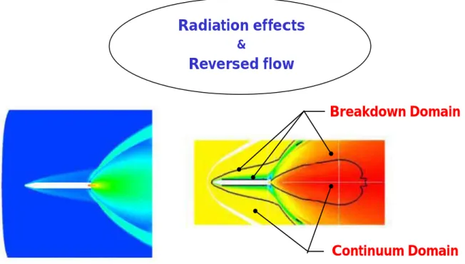
The second example is expanding plumes from a flying projectile at high altitude shown
in Fig. 1.2. There are many complicating phenomena in the upper continuum boost phase
body heating, angle of attack effects, thermal non-equilibrium, dispersion of particulates and
flow interactions from complex flying object geometries. The more important thing is plumes
issuing from those flying objects usually are high temperature gases, thus, reversed flow with
radiation effect may damage the tail of those high speed objects at high altitude. Accurate
predictive tools for the modeling of flying object exhausting plume flows are critical to the
development of high speed flying object related technologies.
Fig. 1.3 shows a sketch of spiral-grooved turbo booster pump (TBP). Spiral-grooved
turbo booster pump has both volume type and momentum transfer type vacuum pump
functions, and is capable of operating at optimum discharge under pressures from
approximately 1000 Pa to a high vacuum. Pumping performance is usually predicted and
examined via traditional CFD methods. However, such the numerical tools are unsuitable
for calculating such rarefied gas region in the highly vacuum chamber. Meanwhile the
computational cost by using a DSMC method in the operation condition with high foreline
pressure (1000 Pa) will be extremely high. Only a hybrid particle-continuum method could
meet both of the above issues with computational efficiency and physical accuracy in both of
the continuum and rarefied gas region.
Configuration of a jet-type CVD reactor is shown in Fig. 1.4. Pulsed Pressure CVD
over traditional CVD technologies and the precursor is delivered in timed pulses into a
continuously evacuated reactor volume. Experimental studies and a phenomenological
model of PP-CVD have shown that during the deposition of titania, the conversion efficiency
of the TTIP precursor into solid film with highly uniform thicknesses exceeds 90% under
certain operational conditions. The unsteady under-expanded jet which forms during the
injection phase contains high property gradients in the shock structure. Consequently during
a pulse cycle the flow contains regions in the continuum, transition and rarefied regimes.
This makes modelling the process extremely challenging, since the validity of continuum
techniques is questionable and particle based techniques such as DSMC are extremely
computationally expensive. In order to continue to develop this promising technology, a
greater understanding of the flow dynamics of the unsteady pulsed pressure regime in
PP-CVD is required.
These above problems can not solved only by either particle method or continuum
method. Thus, it is necessary to develop a proper simulation tool or practical strategy while
considering both of solution accuracy and computational efficiency while involving
continuum and rarefied regions.
1.1.1 Classification of Gas flows
the mean free path traveled by molecules before collision and L is the flow characteristic
length. Flows are divided into four regimes as follows in general: Kn <0.01 (continuum),
0.01<Kn<0.1 (slip flow), 0.1<Kn<3 (transitional flow) and Kn>3 (free molecular flow).
Figure 1.5 shows the various flow regions based on Knudsen number and their corresponding
solution methods in a dilute gas. The local Kn number is defined with L as the scale length
of the macroscopic gradient; that is,
dx d L
ρ ρ
= . As shown in the lower bar, when the local Kn number approaches zero, the flow reaches inviscid limit and can be solved by Euler
equation. Molecular nature of the gas becomes dominated in the flow of interest with the
increase of local Kn increases. When the Kn larger than 0.1, continuum assumption begins
to break down and the particle-based method is necessary. That’s why that the Navier-Stoke
equation based computational fluid dynamics (CFD) techniques will not be adopted while the
Kn are greater that 0.1. The top bar in this figure also shows the validity of the molecular
modeling in the microscopic formulation. It indicates the Boltzmann equation is valid for all
flow regimes. It is well known that Boltzmann equation is more appropriate for all flow
regimes; it is, however, rarely used to numerically solve the practical problems because of
two major difficulties: 1) Higher dimensionality (up to seven) of the Boltzmann equation and
2) difficulties of modeling the integral collision term.
Direct Simulation Monte Carlo (DSMC), proposed by Bird, is an alternative method to
associated monograph was published in [Bird, 1976] and [Bird, 1994]. It is demonstrated
that the DSMC method is equivalent to solving the Boltzmann equation as the simulated
particle numbers become large by both Nanbu [1986] and Wagner [1992]. This method has
been widely used for gas flow simulations in which molecular effects become important.
The advantage of using particle method under these circumstances is that molecular model
can be implemented directly to the calculation of particle collisions without the macroscopic
continuum assumption. Most importantly, DSMC is the only practical way to deal with flows
in the transitional regime, without resorting to the difficult Boltzmann equation, which
requires modeling an integral-differential (collision) term.
1.1.2 Challenge to Particle-Continuum Flow Simulation
For the realistic flows of interest having continuum and continuum breakdown regions,
the direct simulation Monte Carlo (DSMC) method can provide more physically accurate
results in flows having rarefied and non-equilibrium regions than continuum flow models.
However, the DSMC method is extremely computational expensive especially in the
near-continuum region, which prohibits its applications to practical problems with complex
geometries and large domains. In contrast, the computational fluid dynamics (CFD) method,
employed to solve the Navier-Stokes (NS) or Euler equation for continuum flows, is
computationally efficient in simulating a wide variety of flow problems. But the use of
scales (equivalently large Knudsen numbers) can produce inaccurate results due to the
breakdown of continuum assumption or thermal equilibrium. A practical approach for
solving the flow fields having near-continuum to rarefied gas is to develop a numerical model
combining the CFD method for the continuum regime with the DSMC method for the rarefied
and thermal non-equilibrium regime. A well-designed hybrid scheme is expected to take
advantage of both the computational efficiency and accuracy of the NS solver in the
continuum regime and the physical accuracy of the DSMC method in the rarefied or thermal
non-equilibrium regime.
1.2 Literature Reviews
Aktas and Aluru [2002] proposed a multi-scale method that combines the Stokes
equation solver with the DSMC method, which was used for the analysis of micro-fluidic
filters. The continuum regions were governed by Stokes equations solved by a scattered
point finite cloud method. The continuum and DSMC regions were coupled through an
overlapped Schwarz alternating method with Dirichlet-Dirichlet type boundary conditions.
However, the interface location between two solvers was specified in advance. Garcia et al.
[1999] constructed a hybrid particle/continuum algorithm with an adaptive mesh and
algorithm refinement, which was designed to treat multi-scale flow problems. The DSMC
Navier-Stokes solver. This methodology is especially useful when local mesh refinement
for the continuum solver becomes inappropriate as the grid size approaches the molecular
scales. Glass and Gnoffo [2000] proposed “one-shot” coupled 3-D CFD-DSMC method for
the simulation of highly blunt bodies using the structured grid under steady-state conditions.
CFD is used to solve the high-density blunt forebody flow defining an inflow boundary
condition for a DSMC solution of the afterbody wake flow. Interfacial location between the
CFD and DSMC zones was identified manually after one-shot CFD simulation. Results of
CFD simulation at this interface were then used as the inflow boundary conditions (Dirichlet
type) for the DSMC method in the rarefied regions. Wang et al. [2002] proposed a hybrid
information preservation/Navier-Stokes (IP-NS) method to reduce statistical uncertainties
during the process of coupling. The spatial domain decomposition to both of the particle and
continuum domains is based on the continuum breakdown parameter proposed by Wang and
Boyd [2003]. Since the IP method provides the macroscopic information in each time step,
determination of the continuum fluxes across the interface between the particle and
continuum domains becomes straightforward. This method is potentially suitable for
simulating unsteady flows. However, the advantage of particle method in the regions
involving non-equilibrium disappears because the IP method assumes the simulated flow field
is equilibrium thermally. Furthermore, the breakdown parameter proposed by Wang and
due to the effect of high velocity gradient in the boundary layer regions. Roveda et al. [1998]
also proposed a hybrid Euler-DSMC approach for unsteady flow simulations. Two special
approaches were designed to reduce statistical uncertainties at the interface during the
coupling procedures: 1) use of an overlapped region between the DSMC and Euler zones
and 2) use of a “ghost level structure” to reduce statistical uncertainties. However, cloning
of particles is required in this approach and may be problematic in a particle method such as
DSMC. At present, only one-dimensional and two-dimensional flows were demonstrated in
the literature and extension to parallel or three-dimensional simulation has not been reported
to the best knowledge of the authors.
1.3 Motivation
1.3.1 Key Factors of Hybrid DSMC-NS Scheme
As well-known, rarefaction or thermal non-equilibrium can be correctly modeled by the
DSMC method, while CFD (NS, Euler or Stokes) solver can provide a more efficiently
solution for the computational domain. Thus, a hybrid DSMC-NS method can apply the
concept of spatial domain decomposition to distinguish the computational domain of
rarefaction or thermal non-equilibrium to be modeled by the DSMC method, and the
computational domain of continuum to be solved by the CFD (NS, Euler or Stokes) solver.
breakdown criteria in detecting precisely the degree of continuum breakdown in the whole
computational domain. Correct detection of breakdown regions not only guarantees a
physically correct simulation but also prevents the unnecessary computational waste (using
DSMC method in continuum flow regions). It is expected to design some criteria that can be
used to efficiently and accurately identify the breakdown regions and be easily evaluated
during runtime; 2) Comeliness in locating spatial domain boundaries for either DSMC or
continuum method during computation. The location of domain boundaries for DSMC and
continuum domains are identified based on the breakdown regions of the whole
computational domain considering the boundary iterative efficiency during the coupling
process. Coupling strategies, e.g. overlapping region between the continuum and particle
domains, should be used to help the convergence on the hybrid interface for a efficient
simulation; 3) Properly and efficiently exchanging interfacial information (or flow
properties) during runtime. In practice, one side of the interface is the DSMC method with
accuracy strongly depending upon the sampling statistics. The computational efficiency and
accuracy of the continuum solver can be potentially jeopardized by the possibly noisy
boundary conditions if the uncertainty of statistical sampling is large; 4) The effect of
steadiness of the flow solution on designing data exchange at the interface. In the case of
unsteady simulations, the algorithm for data exchange can be very complicated in order to
1.3.2 Continuum Breakdown Parameter
In prior works of continuum breakdown, Bird proposed a semiempirical parameter for
steady-state expanding flows [Bird, 1970]
ds d Ma P ρ ρ λ πγ 8 = (1.1) where Ma is the local march number, γ is the ratio of specific heats and s is the distance
along a streamline. Although it is indicated that the value of P 0.05 is a good criterion for
detecting continuum breakdown in steady flow, the evaluation of the gradient in the
stream-wise direction involves the velocity components to calculate the breakdown
parameter P, it is generally a problem at stagnation points. Furthermore, it is believed that
in complicated flows density is not the only flow property needed to be taken into account.
Wang and Boyd [2003] proposed a new breakdown parameter, which will be introduced
particularly in Chapter 2, to address these issues through the extensive numerical study. It
should be pointed out that the zone of boundary layer is usually indicated as the continuum
breakdown due to the high velocity gradient near the solid wall boundary. However,
molecules which collide on the solid wall with fixed temperature should be thermalized with
the wall temperature based on Maxiwell-Boltzmann distribution. The above concern
motivate us to ponder if the threshold value of continuum breakdown parameter near the
simulation domain accordingly and possibly speed up the convergence of a hybrid method
by not including the boundary layers as part of the continuum breakdown regions. This
necessitates a detailed kinetic study of a well-designed flow problem, in which we can
investigate the continuum breakdown criterion in a more rigorous way.
1.4 Objectives of the Thesis
Based on previous reviews, the objectives of the current study are summarized as
follows.
1) To develop a coupled parallel DSMC-NS method using three-dimensional tetrahedral
or hexahedral unstructured mesh, capable of efficiently and correctly simulating steady
flow.
2) To evaluate and validate the proposed coupled method with supersonic flow over
two-dimension wedge and three-dimensional parallel twin-jets.
3) To revise the continuum breakdown parameter near the solid wall through studying a
kinetic study.
4) To apply the proposed coupled DSMC-NS method to a realistic case which is the study
of plume phenomena from RCS thrusters.
1.5 Organization of the Thesis
mesh, capable of efficiently and correctly simulating steady flows, consisting of both
continuum and rarefied regions is proposed and verified. Steady-state simulations were
performed to reduce the complexity in the coupling process and to verify the present coupled
DSMC-NS method. Possible issues related to the extension of the present approach to
unsteady flows are addressed at the end of the paper.
The present thesis is organized as follows. The particle method (PDSC), the continuum
flow solvers (HYB3D and UNIC-UNS) are introduced in Chapter 2. Details of the proposed
coupled DSMC-NS method are also described in Chapter 2. In Chapter 3, a supersonic
nitrogen flow past a quasi-2-D wedge is chosen as 2-D validation cases for the proposed
coupled method while another realistic 3-D nitrogen flow, which two near-continuum parallel
orifice jets underexpand into a near-vacuum environment, is simulated using the present
coupled method to demonstrate its superior capability. The results and discussions of both
the simulations also summarized. An application of the coupled method that is a study of
plume phenomena of RCS (Rotation Control System) thruster is also simulated by the
coupled method in Chapter 3. By a kinetic study of analyzing the cell velocity samplings,
the continuum breakdown parameter proposed by Wang and Boyd [2003] is reinvestigated
and a new threshold value of the continuum breakdown parameter near the solid wall is also
suggested in Chapter 4. The conclusions and future work of the current study are
Chapter 2
Numerical Methods
2.1 Direct Simulation Monte Carlo
The direct simulation Monte Carlo method (DSMC) [Bird, 1976 and Bird, 1994] is a
particle method for the simulation of gas flows. The gas is modeled at the microscopic level
using simulated particles, which each represents a large number of physical molecules or
atoms. The physics of the gas are modeled through the motion of particles and collisions
between them. Mass, momentum and energy transports between particles are considered at
the particle level. The method is statistical in nature and depends heavily upon
pseudo-random number sequences for simulation. Physical events such as collisions are
handled probabilistically using largely phenomenological models, which are designed to
reproduce real fluid behavior when examined at the macroscopic level. General procedures
of the DSMC method consist of four major steps: moving, indexing, collision and sampling.
In the current study, we use VHS molecular model [Bird, 1976 and Bird, 1994] to reproduce
real fluid behavior as well as no time counter (NTC) [Bird, 1994] for the collision mechanics.
Details of the procedures and the consequences of the computational approximations
regarding DSMC can be found in Bird [Bird, 1976 and Bird, 1994]. In addition, cells in
DSMC are mainly used for particle collision and sampling. Hence, adoption of different
of particle tracking. A special three-dimensional particle ray-tracing technique has to be
designed to efficiently track the particle movement for the special grid system (unstructured)
we use in the current study. The details of the DSMC method and the important features of
PDSC, the parallel generalized three-dimensional DSMC code in the proposed method, will
be introduced later.
2.1.1 General Description of DSMC
Due to the expected rarefaction caused by the very small size of micro-scale devices or
the rarefied gas flows, the current research is performed using the DSMC [Bird, 1976 and
Bird, 1994] method, which is a particle-based method. The basic idea of DSMC is to
calculate practical gas flows through the use of a method that has a physical rather than a
mathematical foundation, although it has been proved that the DSMC method is equivalent to
solving the Boltzmann equation [Nanbu, 1986 and Wagner, 1992]. The assumptions of
molecular chaos and a dilute gas are required by both the Boltzmann formulation and the
DSMC method [Bird, 1976 and Bird, 1994]. The molecules move in the simulated physical
domain so that the physical time is a parameter in the simulation and all flows are computed
as unsteady flows. An important feature of DSMC is that the molecular motion and the
intermolecular collisions are uncoupled over the time intervals that are much smaller than the
mean collision time. Both the collision between molecules and the interaction between
makes extensive use of random numbers. In most practical applications, the number of
simulated molecules is extremely small compared with the number of real molecules. The
general procedures of the DSMC method are described in the next section, and the
consequences of the computational approximations can be found in Bird [Bird, 1976 and Bird,
1994].
In the current study, the Variable Hard Sphere (VHS) molecular model [Bird, 1994] and
the No Time Counter (NTC) [Bird, 1994] collision sampling technique are used to simulate
the molecular collision kinetics. Note that the corresponding molecular data including
reference diameter (dref), reference temperature (Tref), and the viscosity temperature exponent
(ω) for each species are taken from those listed in Ref. [Bird, 1994]. Solid walls for all cases considered in this study are assumed to be fully diffusive (100% thermal accommodation),
unless otherwise specified.
2.1.2 The DSMC Procedures
Fig. 2.1 is a general flowchart of the DSMC method. Important steps of the DSMC
method include setting up the initial conditions, moving all the simulated particles, indexing
(or sorting) all the particles, colliding between particles and sampling the molecules within
cells to determine the macroscopic quantities. The details of each step will be described in
Initialization
The first step to use the DSMC method in simulating flows is to set up the geometry and
flow conditions. A physical space is discredited into a network of cells and the domain
boundaries have to be assigned according to the flow conditions. A point has to be noted is
the cell dimension should be smaller than the mean free path, and the distance of the
molecular movement per time step should be smaller than the cell dimension. After the data
of geometry and flow conditions have been read in the code, the numbers of each cell is
calculated according to the free-stream number density and the current cell volume. The
initial particle velocities are assigned to each particle based on the Maxwell-Boltzmann
distribution according to the free-stream velocities and temperature, and the positions of each
particle are randomly allocated within the cells.
Molecular Movement
After initialization process, the molecules begin move one by one, and the molecules
move in a straight line over the time step. A special particle ray-tracing technique has to be
designed to efficiently track the particle movement for the special grid system, unstructured
grid, which we use in the current study. The particle ray-tracing technique of
3-D Particle Ray-Tracing in Unstructured Mesh
Fig 2.2 is the sketch of the particle movement in three-dimensional unstructured mesh.
The details are described in the following:
Without considering the external force effects, free-flying position of traced particle at
t
t+∆ can be written as, on one hand,
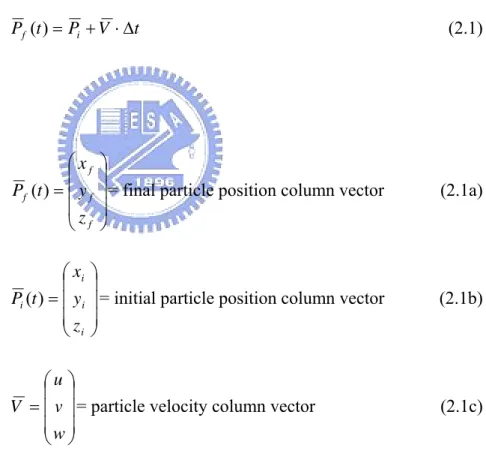
t V P t Pf( )= i + ⋅∆ (2.1) where ⎟ ⎟ ⎟ ⎠ ⎞ ⎜ ⎜ ⎜ ⎝ ⎛ = f f f f z y x t
P ( ) = final particle position column vector (2.1a)
⎟ ⎟ ⎟ ⎠ ⎞ ⎜ ⎜ ⎜ ⎝ ⎛ = i i i i z y x t
P )( = initial particle position column vector (2.1b)
⎟ ⎟ ⎟ ⎠ ⎞ ⎜ ⎜ ⎜ ⎝ ⎛ = w v u
V = particle velocity column vector (2.1c)
On the other hand, cell face can simply be represented as a planar equation as
0
=
+
⋅
p
d
n
(2.2)where n= [a,b,c] is the normal unit vector of the face and P = [x,y,z] is the position vector
) ( ) ( ' cw bv au d cz by ax t i i i + + + + + − = ∆ (2.3)
By computing in turn Eq. (2.3) of each face in the current cell, the correct intersecting
face number can be identified by finding the minimum positive ∆ 't. The intersecting coordinate can be found by substituting ∆ 't into Eq. (2.1). If the intersecting face is a normal face between cells, then the particle will continue its trajectory until it stops.
If the intersecting face is a solid face, the particle will be reflected in a special way (e.g.,
diffusively or secularly) according to the specified boundary condition. These are related by
the coordinate transformation matrix between the local coordinate system (on the face) and
the absolute coordinate system for both types of conditions. First, a unit vector
x
'
alongthe face is chosen, then
y
'
is the cross product ofx
'
andz
'
(the normal unit vector of theface)
'
'
'
z
x
y
=
×
(2.4)The coordination transformation matrix H , is
⎥
⎥
⎥
⎦
⎤
⎢
⎢
⎢
⎣
⎡
=
'
'
'
z
y
x
H
(2.5)transformation −1
H can be easily written as
1 −
H =HT (2.6)
where T
H is the transpose matrix of H .
Now, the particle velocity can be transformed from the velocity in absolute coordinate
system (Vabs) to the velocity in local coordinate system (Vloc) before the reflection by using
H .
loc
V =
H
V
abs (2.7)After the reflection of the particle, the new local coordinate system velocity (Vloc') can be
written as
=
'
loc
V F(Vloc, wall condition) (2.8)
where F(Vloc, wall condition) is a kernel function, depending upon the wall condition and
velocity before reflection.
Finally, the absolute velocity after the reflection ( '
abs
V ) will be obtained by using the
inverse transformer as ' ' 1 ' loc T loc abs H V H V V = − = (2.9)
Indexing
The location of the particle after movement with respect to the cell is important
information for particle collisions. The relations between particles and cells are reordered
according to the order of the number of particles and cells. Before the collision process, the
collision partner will be chosen by a random method in the current cell. And the number of
the collision partner can be easy determined according to this numbering system.
Gas Phase Collisions
The other most important phase of the DSMC method is gas phase collision. The
current DSMC method uses the no time counter (NTC) method to determine the correct
collision rate in the collision cells. The number of collision pairs within a cell of volume Vc
over a time interval ∆t is calculated by the following equation;
c r T N c t V F N N ( ) / 2 1 max∆ σ (2.10)
N and N are fluctuating and average number of simulated particles, respectively.
N
F is the particle weight, which is the number of real particles that a simulated particle
represents. σ and T cr are the cross section and the relative speed, respectively. The
max ) /( )
(σTcr σTcr (2.11)
The collision is accepted if the above value for the pair is greater than a random fraction.
Each cell is treated independently and the collision partners for interactions are chosen at
random, regardless of their positions within the cells. The collision process is described
sequentially as follows:
1. The number of collision pairs is calculated according to the NTC method, Eq. (2.10),
for each cell.
2. The first particle is chosen randomly from the list of particles within a collision cell.
3. The other collision partner is also chosen at random within the same cell.
4. The collision is accepted if the computed probability, Eq. (2.11), is greater than a
random number.
5. If the collision pair is accepted then the post-collision velocities are calculated using
the mechanics of elastic collision. If the collision pair is not to collide, continue
choosing the next collision pair.
6. If the collision pair is polyatomic gas, the translational and internal energy can be
redistributed by the Larsen-Borgnakke model [1975], which assumes in equilibrium.
The collision process will be finished until all the collision pairs are handled for all cells
Sampling
After the particle movement and collision process finish, the particle has updated
positions and velocities. The macroscopic flow properties in each cell are assumed to be
constant over the cell volume and are sampled from the microscopic properties of each
particle within the cell. The macroscopic properties, including density, velocities and
temperatures, are calculated in the following equations [Bird, 1976 and Bird, 1994];
nm = ρ (2.12a) ' c c c co = = o + (2.12b) ) ' ' ' ( 2 1 2 3 2 2 2 w v u m kTtr = + + (2.12c) ) ( 2 r rot rot k T = ε ζ (2.12d) ) ( 2 v v v k T = ε ζ (2.12e) ) 3 ( ) 3
( tr rot rot v v rot v
tot T T T
T = +ζ +ζ +ζ +ζ (2.12f)
n, m are the number density and molecule mass, receptively. c, co, and c’ are the total
velocity, mean velocity, and random velocity, respectively. In addition, Ttr, Trot, Tv and Ttot
the rotational and vibrational energy, respectively. ζrot and ζv are the number of degree
of freedom of rotation and vibration, respectively. If the simulated particle is monatomic gas,
the translational temperature is regarded simply as the total temperature. Vibrational effect
can be neglect if the temperature of the flow is low enough.
The flow will be monitored if steady state is reached. If the flow is under unsteady
situation, the sampling of the properties should be reset until the flow reaches steady state.
As a rule of thumb, the sampling of particles starts when the number of molecules in the
calculation domain becomes approximately constant.
2.1.3 Parallel DSMC Code PDSC
In the proposed coupled DSMC-NS method, PDSC (Parallel Direct Simulation Monte
Carlo Code), developed by Wu’s group [Wu and Tseng, 2005, Wu and Lian, 2003, Wu et al.,
2004a and Wu et al., 2004b], is the 3-D DSMC code used for rarefied and thermally
non-equilibrium regions. Important features of the PDSC code can be found in the
references [Wu and Tseng, 2005, Wu and Lian, 2003, Wu et al., 2004a and Wu et al., 2004b]
and are briefly described in the following.
3-D unstructured-grid topology
Computational cost of particle tracking for the unstructured mesh is generally higher than that
for the structured mesh. However, the use of the unstructured mesh, which provides
excellent flexibility of handling complicated boundary conditions (geometries and varieties)
and of parallel computing using dynamic domain decomposition based on load balancing, is
highly justified.
Parallel computing using dynamic domain decomposition
Load balancing of PDSC is achieved by repeatedly repartitioning the computational
domain using a multi-level graph-partitioning tool, METIS [Karypis and Kumar, 1998 and
Karypis and Kumar, 2003], by taking advantage of the unstructured mesh topology employed
in the code. A decision policy for repartition with a concept of Stop-At-Rise (SAR) [Nicol
and Saltz, 1988] or constant period of time (fixed number of time steps) can be used to decide
when to repartition the domain. Capability of repartitioning of the domain at constant or
variable time interval is also provided in PDSC. Resulting parallel performance is excellent
if the problem size is comparably large. Details can be found in Wu and Tseng [2005].
Variable time-step scheme
PDSC employs a variable time-step scheme (or equivalently a variable cell-weighting
scheme) [Wu et al., 2004a], based on particle flux (mass, momentum, energy) conservation
number of iterations towards the steady state, and the required number of simulated particles
for an acceptable statistical uncertainty. Past experience shows this scheme is very effective
when coupled with an adaptive mesh refinement technique.
2.2 Navier-Stokes Method
Computational Fluid Dynamics have been well developed to numerically solve the
Navier-Stokes equations during the past few decades. Unstructured grid methods are
characterized by their ease in handling completely unstructured meshes and have become
widely used in computational fluid dynamics. The relative increase of computer memory
and CPU time with unstructured grid methods is not trivial, but can be offset by using parallel
techniques in which many processors are put together to work on the same problem.
Traditionally, numerical methods developed for compressible flow simulations use an
unsteady form of the Navier-Stokes or Euler equations. In general, either density or pressure
(density-based or pressure-based) is chosen as one of the primary variables when building up
the discretized governing equations. However, the density-based method in cases of
incompressible or low Mach number flows is questionable, since in low compressibility limit,
and the pressure-density coupling becomes very weak. For flows for all speed regimes,
there are some important researches reported by Hirt et al. [1989], Karki and Patankar [1989]
Koomullil et al., 1996b, Koomullil et al., 1996c, Koomullil and Soni, 1999], are used as flow
solver of continuum flow region in the first phase of developing a coupled method. Then,
the UNIC-UNS code [Chen,1989, Shang et al.,1995a, Shang et al., 1995b, Shang et al., 1995c,
Shang et al., 1997 and Zhang et al., 2001] developed by Chen has been used as the continuum
domain solver in the current couple method instead of HYB3D code because of its powerful
capabilities in handling flows of interest involving low-speed (or incompressible) region, slip
boundary condition and chemical reactions.
2.2.1 General Description of Navier-Stokes Method
The continuum method, employed to solve the Navier-Stokes (NS) or Euler equation for
continuum flows, is computationally efficient in simulating a wide variety of flow problems.
In general, numerical methods developed for compressible flow simulations use an unsteady
form of the Navier-Stokes or Euler equations. The general form of mass conservation,
Navier-Stokes equation, energy conservation and other transport equations can be written in
Cartesian tensor form:
φ φ φ µ φ ρ ρφ S x x U x t j j j j + ∂ ∂ ∂ ∂ = ∂ ∂ + ∂ ∂ ) ( ) ( ) ( (2.13)
where µφ is an effective diffusion coefficient,S denotes the source term, ρ is the fluid φ
energy and turbulence equations, respectively. Detailed expressions for the k-ε turbulence
models and wall functions can be found in [Launder and Spalding, 1974]. For spatial
discretization in cell-centered scheme, the transport equations can also be written in integral
form as
Ω
=
Γ
⋅
+
Ω
∂
∂
∫
∫
∫
Ω Ω Ω Γd
S
d
n
F
d
t
ρφ
(2.14)where Ω is the domain, Γ is the domain surface, n is the unit normal in outward
direction and Fis the flux function of the variables φ and ρ. The flux integral formulation in finite volume scheme can be evaluated by the summation of the flux vectors over each face,
j i k j j i F d n F⋅ Γ=
∑
∆Γ∫
= Γ () , (2.15)where k(i) is a list of faces of cell i , Fi,j represents convection and diffusion fluxes
through the interface between cell i and j, and ∆Γ is the cell-face area. j
In the present work, two cell-centered unstructured finite volume methods HYB3D
[Koomullil et al., 1996a, Koomullil et al., 1996b, Koomullil et al., 1996c, Koomullil and
Soni, 1999] and UNIC-UNS [Chen,1989, Shang et al.,1995a, Shang et al., 1995b, Shang et al.,
1995c, Shang et al., 1997 and Zhang et al., 2001] are used as the continuum solver in the
proposed coupled DSMC-NS method and the general features of both Navier-Stokes solver
codes will be introduced briefly and interested readers are referred to Koomullil [Koomullil et
al., 1996a, Koomullil et al., 1996b, Koomullil et al., 1996c, Koomullil and Soni, 1999] and
Chen [Chen,1989, Shang et al.,1995a, Shang et al., 1995b, Shang et al., 1995c, Shang et al.,
1997 and Zhang et al., 2001] for the details.
2.2.2 Navier-Stokes Solvers: HYB3D and UNIC-UNS Code
HYB3D
The HYB3D is a Navier-Stokes solver using a generalized- or an unstructured- grid
topology and has the following important features: 1) Cell-centered finite-volume upwind
scheme for the numerical integration of governing equations, 2) Roe’s approximate Riemann
solver for convective flux evaluation, 3) Parallel computing using message passing interface
(MPI), 4) Laminar or turbulent flow simulation capability with various turbulence models,
and 5) Application of overset grid topology for flow simulation over moving or complex
bodies. Implicit time integration is used with local time stepping, where the maximum
allowable time step in each cell is determined by the CFL condition constrained by advection
and viscous stability criteria. A second order spatial accuracy is achieved using Taylor’s
series expansion and the gradients of the flow properties are computed using a least-square
method. The creation of local extrema during the higher order linear reconstruction is