基於柏林雜訊之可控制隨機性材質生成

國

立

交

通

大

學

多媒體工程研究所

碩

士

論

文

基 於 柏 林 雜 訊 之 可 控 制 隨 機 性 材 質 生 成

Controllable stochastic texture synthesis based on Perlin Noise

研 究 生：鄭惟謙

指導教授：林文杰 教授

基 於 柏 林 雜 訊 之 可 控 制 隨 機 性 材 質 生 成

Controllable stochastic texture synthesis based on Perlin Noise

研 究 生：鄭惟謙 Student：Wei-Chien Cheng

指導教授：林文杰 Advisor：Wen-Chieh Lin

國 立 交 通 大 學

多 媒 體 工 程 研 究 所

碩 士 論 文

A Thesis

Submitted to Institute of MultimediaEngineering College of Computer Science

National Chiao Tung University in partial Fulfillment of the Requirements

for the Degree of Master

in

Computer Science November 2009

Hsinchu, Taiwan, Republic of China

i

基於柏林雜訊之可控制隨機性材質生成

研究生 : 鄭惟謙 指導教授 : 林文杰 博士

國立交通大學

資訊學院多媒體工程研究所

摘 要

柏林雜訊廣泛運用在產生自然現象，例如：雲，火焰，木紋和地形等應用。藉由 加入柏林雜訊增加擾動也可增添動畫的變化度。然而，過去較少的研究是針對控 制柏林雜訊。我們提出一個可以修改和控制柏林函數所生成的雜訊值，並且不會 破壞原有雜訊函數所擁有的統計上的特性。我們可以產生非常貼近使用者需求的 雜訊樣式並且保有原本雜訊函數該有的統計特性。我們將處理的問題運用多層式 最佳化方法，而分層的依據及最佳化順序是由低頻率雜訊到高頻率雜訊。我們的 方法可以輕易的達到整體性或是區域性的控制例如程序化材質樣式控制，並且我 們可以有效率的再產生相似雜訊樣式。 關鍵字: 柏林雜訊函數，程序化材質生成

ii

Controllable Stochastic Texture Synthesis based on Perlin Noise

Student: Wei-Chien Cheng Advisor: Dr. Wen-Chieh Lin

Institute of Multimedia Engineering

College of Computer Science National Chiao Tung University

ABSTRACT

Perlin noise is widely used to render natural phenomena such as cloud, fire, woodgrain and terrain. It is also used to enrich the variety of animation by adding disturbance to the motion of objects. However, there is less attention on controlling Perlin noise in the past. We present a new approach to modify and control the noise value generated by Perlin noise function without destroying the statistical properties of the noise function. We can generate the controllable noise that closely matches a user’s demand pattern while preserving the original statistical properties of noise. We formulate our problem as a multi-level optimization problem in which the optimization process is executed from low frequency level to high frequency level. Our approach can easily achieve global and local control on texture pattern design and can reproduce the same pattern efficiently.

iii

Acknowledgements

I would like to thank my advisor, Professor Wen-Chieh Lin for his guidance, inspirations, useful ideas and encouragement. Thanks to my colleagues in our lab: Kuei-Li Fang, Hsi-Chou Huang, Yi-Jheng Huang, Ting-Chieh Huang, Zhi-Cheng Yan, . Hsuan-Ya Yu, Hong-Xuan Ji, Jau-An Yang, Tsung-Sheng Fu and Chan-Yu Lin for their assistances and discussions. It is honor to work with all of them. Eventually, I would like to thank my parents and my girlfriend for their love and support.

iv

Contents

Introduction ... 1 Related Work ... 5 2.1 Noise Functions ... 5 2.2 Noise Control ... 6 Approach ... 8 3.1 Overview ... 8

3.2 Perlin Noise Function ... 9

3.3 Goodness of Fit Test ... 13

3.3.1 Chi-Square goodness of fit test ... 13

3.3.2 Kolmogorov-Smirnov goodness of fit test ... 14

3.3.3 Comparisons of both tests ... 15

3.4 Noise Optimization Process ... 17

3.4.1 Objective Function ... 17

3.4.2 Multi-Level Optimization ... 18

3.5 Noise Reproduction ... 21

3.5.1 Sampling Optimal Gradient Vectors ... 23

3.5.2 Initial Clustering of Sampled Gradient Vectors... 24

3.5.3 Modeling Gradient Vector Distribution ... 25

Results ... 28

4.1 Control of 2D Textures Synthesis ... 28

4.2 Statistical Analysis ... 33

4.3 Comparison of results under different parameters settings ... 36

4.3.1 Different Starting Frequencies ... 36

4.3.2 Different weightings of the control term and the KS term ... 37

v

4.5 Terrain Generation ... 47

Conclusion and Future Work ... 51 Bibliography ... 54

vi

List of Figures

Figure 1.1: Procedure textures generated by Perlin noise function ... 2

Figure 1.2: Terrain editing by modifying the height at a specific location on (a) original terrain (b) after editing [8] ... 3

Figure 3.1: System Overview ... 10

Figure 3.2: (a) Grid points with assigned gradient vectors. (b) Noise value is interpolated from surrounding dot product value ... 11

Figure 3.3: Fractal sum image composed of different frequencies. ... 12

Figure 3.4: Noise appearance with uniform and non-uniform gradient vectors distribution. ... 13

Figure 3.5: The KS test is based on the maximum distance between these two curves. . ... 15

Figure 3.6: Two situations with the same chi-square error. Each arrow represents a gradient vector and the color distinguish different bins.(a) The gradient vectors in the bin are uniformly distributed, (b) The gradient vectors in the bin are gathered with a non-uniform distribution. ... 16

Figure 3.7: User control pattern. ... 18

Figure 3.8: (a) Low frequency noise controls the global shape of the noise appearance and the (b) high frequency noise controls the detail. ... 19

Figure 3.9: Propagate the gradient from low-freq level to high-freq level as the initial guess. ... 21

Figure 3.10: A sketch of the noise reproducing procedure. ... 22

Figure 3.11: Merge the NQ input data ... 25

Figure 4.1: Thee Cloud textures generated with different user control patterns. ... 29

Figure 4.2: Three Marble textures generated with different control patterns. ... 30

vii

Figure 4.4: Three Fire textures generated with different control patterns. ... 32

Figure 4.5: Comparison of the Chi-square test and KS test. ... 34

Figure 4.6: Comparison of the Chi-square test and KS test. ... 35

Figure 4.7: Stochastic textures of different starting frequency of fractal sum: (a) 𝑓1 = 2 (b) 𝑓1 = 4 (c) 𝑓1 = 6 (d) 𝑓1 = 8... 37

Figure 4.8: Stochastic textures of different control weight (a) 𝑤1 = 0, 𝑤2 = 1 (b) 𝑤1 = 0.1, 𝑤2 = 0.9 (c) 𝑤1 = 0.01, 𝑤2 = 0.99 (d) 𝑤1 = 0.001, 𝑤2 = 0.999 (e) 𝑤1 = 0.0001, 𝑤2 = 0.9999 (f) 𝑤1 = 0.00001, 𝑤2 = 0.99999 ... 38

Figure 4.9: The reproduced erosion texture and the original texture by optimization. List the KS error and the control term error in the right column. ... 40

Figure 4.10: CDF comparison between Original and Reproduced Noises, plot the .... 41

Figure 4.11: The reproduced marble texture and the original texture by optimization. List the KS error and the control term error in the right column. ... 42

Figure 4.12: CDF comparison between Original and Reproduced Noises, plot the curves together and the curve is approximated to the original CDF. ... 43

Figure 4.13: The reproduced cloud texture and the original texture by optimization. List the KS error and the control term error in the right column. ... 44

Figure 4.14: CDF comparison between Original and Reproduced Noises, plot the .... 45

Figure 4.15: Terrain height map generated by user-specified flower pattern. ... 48

Figure 4.16: Terrain height map generated by user-specified “X” pattern. ... 49

Figure 4.17: Terrain height map generated by user-specified star pattern. ... 50

Figure 4.18: Stochastic texture synthesis applied in 3D application. ... 52

viii

List of Tables

Pseudo code 3.1: The algorithm of multi-level optimization ... 20

Pseudo code 3.2: Noise Reproducing Procedure ... 27

Table 4.1: The parameters used in GMM fitting for erosion texture ... 41

Table 4.2: The parameters used in GMM fitting for marble texture ... 43

Table 4.3: The parameters used in GMM fitting for cloud texture ... 45

1

Chapter 1

Introduction

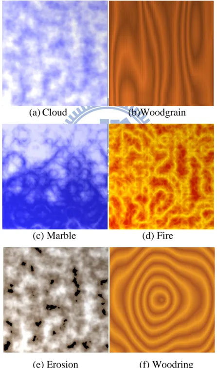
Noise functions are commonly used in computer graphics. It is used to create complex natural phenomenon and generate procedural texture as shown in Figure 1.1. Acquiring a noisy appearance by simply sampling a random number generator for every point would not be appropriate, since the appearance is too random. Instead, we would like the noise to be smoother and without losing the random property. The noise function introduced by Ken Perlin [1,2] is a well-established method for random number generator. There are several functions to generate random numbers. However, the problem is that those functions are not continuous at all. The Perlin noise is a well-known generator which gives random numbers that are almost continuous, furthermore, it is not only used as a primitive operation to create procedural texture and shading but also as an approach to create natural and realistic animation by adding some random disturbance to a motion. Unlike white noise which is composed of unconstrained random number, Perlin constructs noise from different bands and each band is limited to a range of frequencies. By summing up different noise bands weighted by amplitude, we can produce a variety of pattern such as wood, marble, cloud etc [4] (Fig.1.1) and provide more natural looking. Perlin noise function is

2

simple, efficient and provides adequate spectral control, so it is still the most popular approach in computer graphics. The ideal noise function should have following properties: band-limited, stationary, isotropic, reproducible, and not periodic. These properties have motivated researchers on improving the noise quality by developing more precise random number table to reduce the bias and band-limited.

(a) Cloud (b)Woodgrain

(c) Marble (d) Fire

(e) Erosion (f) Woodring

3

Although, computer graphics researchers have proposed various applications by composing multiple noises to describe a complex pattern or natural phenomenon, there is less attention on controlling the noise functions. This is because modifying on the noise value arbitrarily will destroy the ideal properties of the noise function. Some applications, such as procedural texture synthesis and terrain synthesis need to specify noise values to generate a pattern that meets the user’s demands. Figure 1.2 shows an example of terrain editing in which the noise values are used as a map of height filed and we can assign the noise value in some positions of this map to generate the demanded terrain.

(a) (b)

Figure 1.2: Terrain editing by modifying the height at a specific location on (a) original terrain (b) after editing [8]

In this thesis, we propose an approach, targeted at interactive application, to generate controllable noise that closely matches a user’s demand value without losing its original properties through an optimization process. Furthermore, we can make the controllable noise function reproducible without re-running lengthy optimization by sampling the distribution of the random number tables that fulfill the user-specified pattern and statistical properties. The contributions of this thesis are:

 Proposing an approach that can generate a user-demanded noise pattern through an optimization process while preserving the statistical properties of the random number table.

4

 Developing a multi-level optimization algorithm that can effectively reduce the computational time by propagating the optimizing values from lower levels to higher levels.

 Reproducing the same noise patterns without re-running the computationally expensive optimization process.

The rest of the thesis is organized as follows: Chapter 2 reviews previous work: on noise functions and related work on controlling noise generation. Chapter 3 briefly introduces the background of Perlin noise function and describes our approach to generate a controllable and reproducible noise function. Chapter 4 shows our experimental results. Finally, conclusion and future work are discussed in Chapter 5.

5

Chapter 2

Related Work

In this chapter, we give a brief introduction about Perlin noise and related applications of noise function researches in section 2.1 and review some methods of controlling noise in section 2.2.

2.1 Noise Functions

Perlin [1,2] introduced the noise function that can be used to generate procedural textures [4,5,6] such as cloud, marble, fire, woodgrain and etc. Besides, it can be used to disturb the movement of an object to make animated motions look more natural [10]. Perlin and Neyret [15] suggested a method to carry out swirling and flowing time varying texture by rotating the gradient and making pseudo-advection by sampling the noise with an offset. With programmable graphics hardware, Perlin noise has been implemented on GPU shader [3] who developed a general purpose multipass pixel shader to generate the Perlin noise function. Lewis [11] proposed another approach to generate natural pattern based on Wienner interpolation. His approach can generate noise with arbitrary energy spectrum, but his method is more complicated than Perlin’s method. Cook and DeRose [13] pointed out that Lewis’

6

approach is insufficient to solve the loss-of-detail and aliasing problem. They propose the wavelet analysis to construct noise bands for anti-aliasing and achieve band-limited by eliminating unnecessary low frequencies. Goldberg et al. [14] introduced a method that provides high quality anisotropic filter for noise textures. They generated noise directly on frequency domain partitioned into oriented subbands and approximated noise with desired spectrum. Perlin [4] introduced an improved algorithm that solved two problems in the original Perlin noise function [1,2]: One is second order interpolation discontinuity and the other is non-optimal gradient distribution which might cause directional bias. He proposed a new interpolation that gives c2 continuity. To prevent the gradient distributed non-uniformly and speed up the computation, Perlin suggested a new gradient table containing only 16 vectors. However, the 16 gradient vectors are fixed and insufficient to satisfy the user-demanded noise value.

2.2 Noise Control

There have been few approaches dealing with the controllability of noise functions. Lewis [12] proposed the stochastic subdivision construction which provides control of the autocorrelation and spectral properties of the synthesized random functions. The stochastic techniques can model a variety of natural and complex phenomenon. Ebert et al. [4] introduced different types of noise function implementation. Yoon et al. [8] proposed a method to control Perlin noise by modifying the pseudo-random gradient table for satisfying users’ demand. They use the Chi-Square test to preserve the uniform distribution of the random number table while modifying the element of the table. However, they only considered the composition of the modified noise value as their optimized variables; their approach can just achieve local control. Later, Yoon et al. [25] proposed a method that can extract patterns from existing objects by non-uniform noise functions and use it to generate procedural textures. Yoon et al. [9] integrated other statistical tools to measure the stability of a random number table during an optimization process to meet the user specified pattern. Their method can maintain the property of the noise

7

function including uniform distributed, non-periodic and band-limited. They also introduced a stochastic tiling approach using Wang tiles [16] to accelerate the generation of the random number table. These two approaches proposed by Yoon et al. [8,9] above cannot achieve reproducibility because they need to run the optimization procedure repeatedly to generate the same noise pattern. It is time-consuming. Therefore, we proposed an approach to generate the similar noise pattern in real-time in this thesis.

8

Chapter 3

Approach

This chapter describes our algorithm for generating user-defined noise and reproducing the controlled noise pattern without re-optimization. First, we give an overview of our approach in section 3.1. Second, we describe the background of Perlin noise function, including the composition of Perlin noise function and rewriting the noise function into a simpler form for control. Finally, we describe the details of our algorithm, including the goodness of test for maintaining the uniform distribution of the gradient vectors (section 3.2), the optimization process (section 3.3) and the noise reproducing approach (section 3.4).

3.1 Overview

The goal of our approach is to control the generation of the noise value as much similar as user-defined pattern; however, modifying the components of the noise composition arbitrarily might violate required statistical property of Perlin noise. To achieve our goal, we develop a multi-level optimization process to obtain noise which does not only preserve statistical properties but also closely match user-specified noise patterns.

9

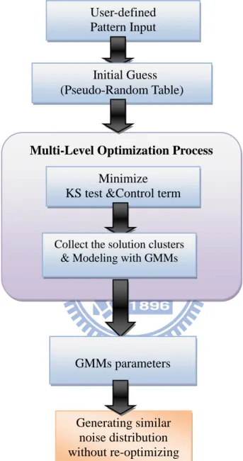
Figure 3.1 shows an overview of our approach, which can be divided into two stages: the preprocessing stage and the noise reproducing stage. In the preprocessing stage, the input of our system is a user-specified pattern image. Our system extracts the user controls and uses them as the initial guess of the optimization solver. Then, the optimization process will keep the user-specified noise with the statistical properties. Since the fractal sum of noise is composed of low to high frequency noise, the gradient vectors are shared by low to high frequency noise. We applied a hierarchical framework of optimization to reduce the computational time. We classify the gradient vector in accordance with which belongs to low frequency or high frequency noise for our optimizing order. Once we get the optimized gradient vectors (the component of the noise composition), we estimate the gradient vector distribution so that we can resample the gradient vectors from the estimated distribution model without re-running optimization. We apply the hierarchical clustering algorithm that clusters the optimized solutions to get an initial guess of the number of component in the Gaussian mixture model. We iteratively use Gaussian mixture model to fit our solution set until we get the appropriate number of component in order to reproduce the same pattern of noise. In the next stage, we can real-time reproduce the similar pattern noise without losing the statistical properties.

3.2 Perlin Noise Function

As our method is based on Perlin noise function[1, 2], we introduce the background of Perlin noise function and derive the noise function into a more definite form for our optimization problem.

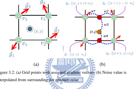
Perlin noise function is known as lattice noise. This function uses a hypercubic lattice on which a gradient vector is assigned at each grid point (see Figure. 3.2(a)). The noise value between grid points is obtained by interpolating the noise values at the surrounding grid points (Figure 3.2(b)).We store the gradient vectors in a gradient table G, and a permutation table P for hashing indices. The number of lattice points for each noise value is determined by the dimension of noise function, for example, 2D noise requires 22 gradient vectors and 3D noise requires 23 gradient vectors so

10

that N-dimensional noise requires 2N gradient vectors to compute a noise value. We summarize the noise generating operation below:

Figure 3.1: System Overview

Step 1: Precompute the unit length gradient vectors which store in the G table with

size M and precompute P table of size M called permutation table which stores the integer random number from 0 to M-1.

Step 2: Acquire 2N _{sets of grid point coordinates. In 2D case for instance, we obtain}

Multi-Level Optimization Process

User-defined Pattern Input

Initial Guess (Pseudo-Random Table)

Minimize KS test &Control term

Generating similar noise distribution without re-optimizing

optimization

Collect the solution clusters & Modeling with GMMs

11

22 _{integer points 𝑣}

1 = 𝑥 , 𝑦 , 𝑣2 = 𝑥 + 1, 𝑦 , 𝑣3 = 𝑥 , 𝑦 + 1 , 𝑣4 =

𝑥 + 1, 𝑦 + 1 (see Fig 3.2). The four integer grid points form an unit quadrangle surrounded the input point (𝑥,𝑦). Hence, we acquire four unit gradient vectors from the G table hashing by the indices ( 𝑥 , 𝑦 ) through the P table 𝑔 ₁ = 𝐺[𝑃 𝑃 𝑥 + 𝑦 ] (see Fig 3.2(b)) and the other three gradient vectors 𝑔 ₂, 𝑔 ₃, 𝑔 ₄ may obtain as the same operation.

(a) (b)

Figure 3.2: (a) Grid points with assigned gradient vectors. (b) Noise value is interpolated from surrounding dot product value

Step 3: In 2D case, the noise value is interpolated by the four dot products (see Fig

3.2(b)). The dot product is operated as 𝑔 ₁∙ 𝑥, 𝑦 − 𝑣₁ and the other three grid noise values will be obtained. We used the improved ease curve 𝑤 𝑡 = 6 𝑡 5− 15 𝑡 4+ 10 𝑡 3 [7] instead of the original Perlin’s method to compute the weight. In the next section, we will formulate the above concept and derive the noise function to deal with our optimization problem.

As show in Figure 3.2(b), noise value is the combination of its surrounded dot product value at grid point. In 2D case, we can easily formulate as below:

𝑁𝑜𝑖𝑠𝑒 𝑥, 𝑦 = 𝑤(𝑥 − 𝑖)𝑤(𝑦 − 𝑗)(Δ _𝑖𝑗 ∙ 𝐺 _𝑖𝑗) 𝑦 +1 𝑗 = 𝑦 𝑥 +1 𝑖= 𝑥 (3.1)

12

We define Δ 𝑖𝑗 = (𝑢, 𝑣) = (𝑥 − 𝑖, 𝑦 − 𝑗) where 𝑤(𝑥 − 𝑖)𝑤(𝑦 − 𝑗)(Δ 𝑖𝑗 ∙ 𝐺 𝑖𝑗) can be

represented as 𝑤(𝑢)𝑤(𝑣)(Δ 𝑖𝑗 ∙ 𝐺 𝑖𝑗), G 𝑖𝑗 denotes the gradient vector hashing by the

indices 𝑖, 𝑗 and the weighting function 𝑤 𝑡 = 1 − (6 𝑡 5− 15 𝑡 4+ 10 𝑡 3). For convenience, we merge the 𝑤(𝑢)𝑤(𝑣)(Δ 𝑖𝑗) into a vector representation 𝑊 𝑖,𝑗, so the

noise function can represent as a combination of four dot products below:

𝑁𝑜𝑖𝑠𝑒 𝑥, 𝑦 = 𝑊 _𝑖,𝑗 ∙ 𝐺 _𝑖,𝑗 + 𝑊 _{𝑖,𝑗 +1}∙ 𝐺 _{𝑖,𝑗 +1} + 𝑊 _𝑖+1,𝑗 ∙ 𝐺 _𝑖+1,𝑗 + 𝑊 _{𝑖+1,𝑗 +1}∙ 𝐺 _{𝑖+1,𝑗 +1}

To express the natural-looking phenomenon, we need the noise function to be smooth and random. Therefore, we sum up several frequencies of noise called fractal sum. It is composed of low frequency noise with higher amplitude and high frequency with lower amplitude. Figure 3.3 shows the fractal sum noise appearance. The fractal sum is defined as follows:

where 𝐹 is called "octave",𝑓𝑖 is the weight of frequency and 𝑎𝑖 is the weight of

amplitude. The coefficients own the following properties. 𝑓_𝑖 < 𝑓_𝑖+1 and 𝑎_𝑖 < 𝑎_𝑖+1 and usually two times larger than the previous one.

Figure 3.3: Fractal sum image composed of different frequencies.

(3.2) (3.3) 𝐹_𝑠𝑢𝑚 = 𝑁𝑜𝑖𝑠𝑒(𝑓𝑖𝑥, 𝑓𝑖𝑦)) 𝑎_𝑖 𝐹 𝑖=1

13

3.3 Goodness of Fit Test

As the above section described, the N dimension noise value is composed of

N

2 dot products. Since our goal is to modify the gradient vectors in the G table to match the user-specified noise value, we need to use some statistical tools to maintain the gradient vectors distribution uniformly. Figure 3.4 shows the comparison between the non-uniform and the uniform gradient distribution. As shown, bias distribution might cause the artifacts with the noise appearance. Consequently, we should exploit the statistical tool to assess the uniformity of the gradient distribution.

The goodness of fit of a statistical model is used to describe how well the observed data fits the expected distribution. We adopt goodness of fit test to compare the observed data with the desired distribution. Instead of using Chi-Square goodness of test [8, 24], we adopt Kolmogorov-Smirnov goodness of fit proposed by Massey [17]. We will introduce both methods in section and explain the reason why we replace Chi-Square test with Kolmogorov-Smirnov test (KS test) in section 3.3.3.

(a)Uniform distribution (b) Non-uniform distribution Figure 3.4: Noise appearance with uniform and non-uniform gradient vectors distribution.

3.3.1 Chi-Square goodness of fit test

14

two distributions based on their sample data and determine if the sample data comes from a specified distribution. Let 𝑋 = {𝑋₁, 𝑋₂, 𝑋₃… … , 𝑋_𝑀 } be the observed 𝑀 data. To compute the distribution from observed data, we divide the set 𝑋 into 𝐾 bins and define 𝑂𝑘 as the set of observed data in the 𝑘𝑡𝑕 bin. Let 𝐸 be the specified

distribution and 𝐸_𝑘 be the observed distribution for the 𝑘_𝑡𝑕 bin. Thus, the Chi-square test measuring the similarity between the set 𝑂 and set 𝐸 is defined as follows:

𝐶𝑆(𝑋, 𝐸) = ( 𝑂_𝑘 − 𝐸_𝑘 )2_{/ 𝐸} 𝑘 𝐾

𝑘=1

where 𝑂𝑘 is the number of observed data in the 𝑘𝑡𝑕 bin and 𝐸𝑘 denotes the

number of samples in the 𝑘_𝑡𝑕 bin. For Perlin noise, we need the direction of gradient vectors to be uniformly distributed. Thus, we divide the data 𝑋 into 𝐾 bins with the same 𝐸𝑘 which equals to 𝑀/𝐾 . 𝐶𝑆 is the difference between the observed

distribution and specified distribution. Hence, the smaller a 𝐶𝑆 value is, the better the distribution of observed data matches the specified distribution. But how to decide the value K and there are some limitations and disadvantages on Chi-Square test, we

will explain in section 3.3.3 later.

3.3.2 Kolmogorov-Smirnov goodness of fit test

The

Kolmogorov-Smirnov goodness of fit test (KS test) is used to determine whether a sample comes from a population with a specific distribution. The KS test quantifies the distance between the empirical distribution function of the sample and the empirical distribution function of the specified distribution. It is formed as a minimum distance estimation as below:

𝐾𝑆 𝑋, 𝐸 = 𝑀𝑎𝑥 𝐹𝑋 𝑥 − 𝐹𝐸(𝑥)

(3.4)

15

where 𝐹_𝑋 is the empirical distribution function which is a cumulative probability distribution function for M independent and identically distributed observations 𝑋_𝑖 defined as below:

𝐹_𝑀 𝑥 = 1

𝑀 𝐼(𝑋𝑖 ≤ 𝑥)

𝑀

𝑖=1

where 𝐼(𝑋𝑖 ≤ 𝑥) is the indicator function which equals to 1 if 𝑋𝑖 ≤ 𝑥 and equals to

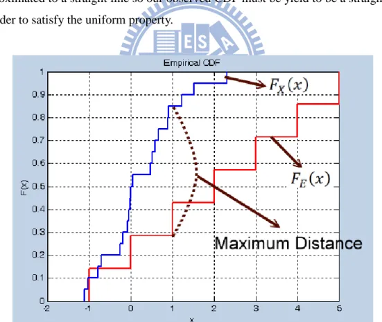
0 otherwise. Figure 3.5 indicates the concept of the KS test. If the observed distribution matches the specified distribution, the curve of the cumulative distribution function (CDF) might be similar. Thus, the maximum distance between the two curves must be very small. In the uniform distribution case, the curve of the CDF is approximated to a straight line so our observed CDF must be yield to be a straight line in order to satisfy the uniform property.

Figure 3.5: The KS test is based on the maximum distance between these two curves.

3.3.3 Comparisons of both tests

16

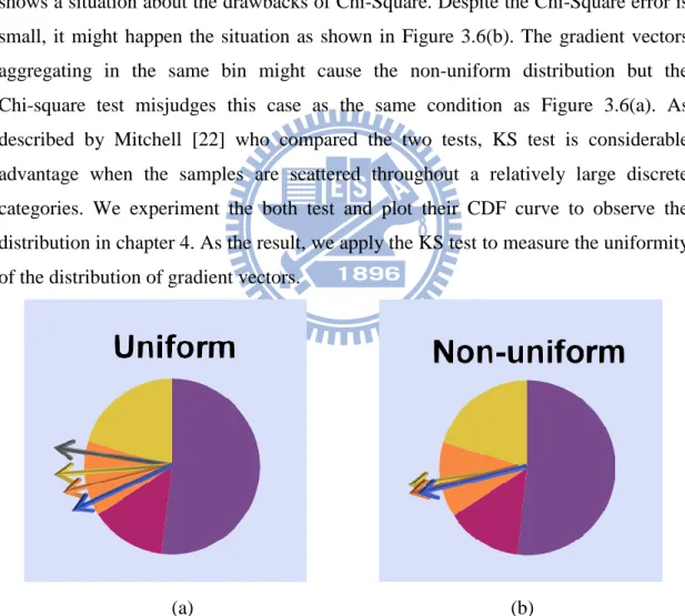
In this section, we explain why we adopt KS test instead of Chi-Square test. There are some drawbacks in those two tests. KS test is confined to one- and two- sample condition, whereas Chi-Square test can be extended to k sample condition. In our case, we just compare two distributions so the limitation of the KS test is not an issue. Besides, the Chi-square test requires the expected number in each bin sufficiently large. It is often accepted that each bin have an expected number greater or equal to 5 [19, 20, 21]. KS test does not have the restriction of expected number associated with Chi-Square test. Although the Chi-Square error might be small, it cannot ensure that the distribution of the gradient vectors is truly uniform. Figure 3.6 shows a situation about the drawbacks of Chi-Square. Despite the Chi-Square error is small, it might happen the situation as shown in Figure 3.6(b). The gradient vectors aggregating in the same bin might cause the non-uniform distribution but the Chi-square test misjudges this case as the same condition as Figure 3.6(a). As described by Mitchell [22] who compared the two tests, KS test is considerable advantage when the samples are scattered throughout a relatively large discrete categories. We experiment the both test and plot their CDF curve to observe the distribution in chapter 4. As the result, we apply the KS test to measure the uniformity of the distribution of gradient vectors.

(a) (b)

Figure 3.6: Two situations with the same chi-square error. Each arrow represents a gradient vector and the color distinguish different bins.(a) The gradient vectors in the bin are uniformly distributed, (b) The gradient vectors in the bin are gathered with a non-uniform distribution.

17

3.4 Noise Optimization Process

In the previous section, we described the uniform property of the noise generation. We apply the property as a part of terms in the optimization process. We will describe how we set the objective function for the optimization (section 3.4.1) and extend the optimization to the multi-level hierarchical framework (section 3.4.2).

3.4.1 Objective Function

We applying Kolmogorov-Smirnov goodness of fit test introduced in the section 3.3.2 as a mechanism for preserving the gradient vectors to be uniformly distributed when modifying the gradient vectors. It is a part of terms in our objective function named 𝐸𝐾.𝑆 defined below:

𝐸_𝐾.𝑆 = 𝐾𝑆 𝑋_{𝑖𝑑𝑒𝑎𝑙}, 𝑋_𝑜𝑏𝑠 = 𝑀𝑎𝑥 𝐹𝑖𝑑𝑒𝑎𝑙 𝑥 − 𝐹𝑜𝑏𝑠(𝑥)

where 𝑋_{𝑖𝑑𝑒𝑎𝑙} is the ideal uniform sample set used to compare with the observed 𝑋_𝑜𝑏𝑠 samples. In 2D case, we collect the set 𝑋𝑖𝑑𝑒𝑎𝑙 from the uniform samples in 𝑅2. Since

the length of all gradient vectors is 1, we can represent a vector X = (𝑥, 𝑦) by (𝑐𝑜𝑠𝜃, s𝑖𝑛𝜃). This reduces the dimension of variables in the optimization process.

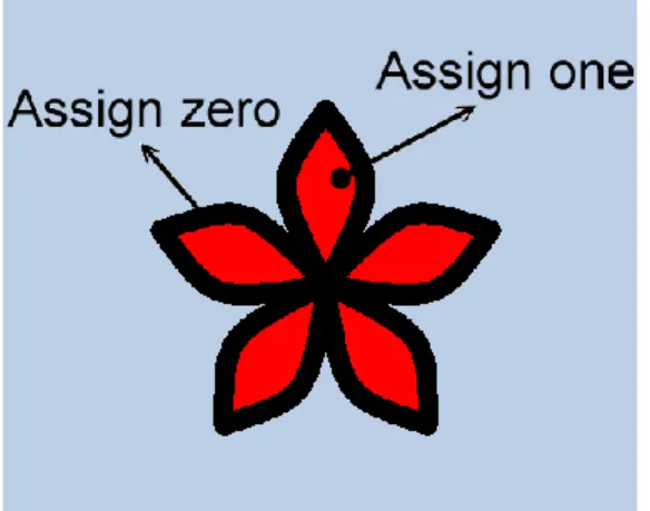
In order to control the noise value, we require applying some controls on the gradient vectors. We simply extract the control information from the user input pattern. As shown in Figure 3.7, black color and red color denote noise value of 0 and 1, respectively. In this thesis, we focus on the 2D case. Thus, the noise function can represent as Equation 3.2. Let 𝑉_𝑖= 𝑁𝑜𝑖𝑠𝑒 𝑥_𝑖, 𝑦_𝑖 and 𝐷_𝑖 be the noise value to be optimized and user-specified noise value, respectively. The user-control term in our objective function is defined as follows.

𝐸_𝐶𝑜𝑛 = (𝑉_𝑖 − 𝐷_𝑖)2 𝐼

𝑖=0

(3.7)

18

Figure 3.7: User control pattern.

where 𝐼 denotes the total number of user-specified noise values. Therefore, we can define our objective function 𝐸 as below:

𝐸 = 𝑤₁𝐸_𝐾.𝑆+ 𝑤₂𝐸_𝐶𝑜𝑛

where 𝑤1 and 𝑤2 are the control weight of these two terms to achieve not only the

gradient vectors uniformly distributed but user-demanded control. As our experiment result, we set the 𝑤₁ as 0.995 and 𝑤₂ as 0.005 as the weight value. The Simulated Annealing algorithm that is a method for solving unconstrained optimization problems and it is often used when the search space is discrete. Hence, we apply this algorithm to solve our optimization problem.

3.4.2 Multi-Level Optimization

As described in section 3.2, fractal sum which used to express the natural-looking phenomenon is composed of several frequencies of noise from low frequency noise with higher amplitude and high frequency with lower amplitude. However, we can divide the optimization process into several stages based on this property. As shown in Figure 3.8, low frequency noise controls the global shape of the fractal noise appearance. The low frequency noise uses the fewer gradient vectors due to the grid points contains in low frequency noise are fewer than those in high frequency noise. In low frequency noise, the range of hashing indices ( 𝑓𝑙𝑥 , 𝑓𝑙𝑦 ) is

19

(a) (b)

(c) (d)

Figure 3.8: (a) Low frequency noise controls the global shape of the noise appearance and the (b) high frequency noise controls the detail.

two times smaller than that in high frequency. That is, in low frequency noise the number of the grid points hashing by ( 𝑓_𝑙𝑥 , 𝑓_𝑙𝑦 ) is fewer than in high frequency noise. We simply classify the gradient vectors in accordance with which are shared by low frequency noise and the rest gradient vectors are classified into high frequency noise for our optimizing order. Besides, the gradient vectors corresponding to lower frequency noise will propagate the optimized gradient vectors to the higher frequency level as its initial guess. In this paper, we set the octaves 𝐹 = 4, the start amplitude 𝑎1 = 4 , 𝑓1 = 8 , 𝑓𝑙+1= 2𝑓𝑙 and 𝑎𝑙+1 = 2𝑎𝑙. Therefore, the fractal sum noise

function can be expanded as follow:

𝐹_𝑠𝑢𝑚 = 𝑁𝑜𝑖𝑠𝑒(𝑓𝑙𝑥, 𝑓𝑙𝑦) 𝑎_𝑖

4

𝑙=1

where −1 ≤ 𝑁𝑜𝑖𝑠𝑒(𝑥, 𝑦) ≤ 1 and 𝑙 denotes the level in optimization. Apparently, we can observe that the lowest frequency affect the noise value the most due to the largest weight of this component. Our strategy is that satisfying the lowest frequency (3.10)

20

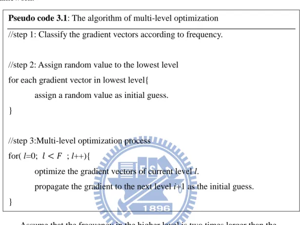
noise value which is prior to higher ones and propagate the gradient vectors to the next higher noise function. Besides, the number of gradient vectors shared by lower level is smaller than the higher one. Pseudo code 3.1 summarizes our hierarchy framework.

Assume that the frequency in the higher level is two times larger than the lower level, we list the gradient vectors shared by the two levels 𝑙 and 𝑙 + 1 as

𝑁𝑜𝑖𝑠𝑒 𝑓_𝑙𝑥, 𝑓_𝑙𝑦 → 𝐺[𝑃[𝑃 𝑓_𝑙𝑥 + 𝑓_𝑙𝑦 ]]

𝑁𝑜𝑖𝑠𝑒 𝑓_𝑙+1𝑥, 𝑓_𝑙+1𝑦) = 𝑁𝑜𝑖𝑠𝑒 2𝑓_𝑙𝑥, 2𝑓_𝑙𝑦) → 𝐺[𝑃[𝑃 2𝑓_𝑙𝑥 + 2𝑓_𝑙𝑦 ]]

we can derive the relation between the adjacent two levels and propagate the gradient vectors as this rule:

𝐺 𝑃 𝑃 𝑓_𝑙+1𝑥 + 𝑓_𝑙+1𝑦 = 𝐺[𝑃[𝑃 (𝑓_𝑙+1𝑥)/2 + (𝑓_𝑙+1𝑦)/2 ]

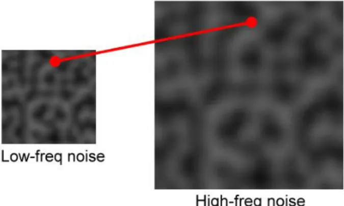
Figure 3.9 shows the schematic diagram of the propagation concept. Since the fractal noise value is cumulated from lower to higher frequency noise, satisfying the lower

Pseudo code 3.1: The algorithm of multi-level optimization

//step 1: Classify the gradient vectors according to frequency.

//step 2: Assign random value to the lowest level for each gradient vector in lowest level{

assign a random value as initial guess. }

//step 3:Multi-level optimization process for( l=0; 𝑙 < 𝐹 ; l++){

optimize the gradient vectors of current level l.

propagate the gradient to the next level i+1 as the initial guess. }

(3.12) (3.11)

21

level ensured that the error between 𝑉_𝑖 − 𝐷_𝑖 might be reduced immensely. Since we propagate the gradient vectors to the higher level as its initial guess, the initial error value is usually smaller than that of the random initial guess. The optimization converges faster due to the more reasonable initial guess.

Figure 3.9: Propagate the gradient from low-freq level to high-freq level as the initial guess.

In each level, we simply modified the KS term and user-control term as below:

𝐸𝑙_𝐾.𝑆 = 𝐾𝑆 𝑋_{𝑖𝑑𝑒𝑎𝑙}, 𝑋𝑙_𝑜𝑏𝑠

𝐸𝑙𝐶𝑜𝑛 = (𝑉𝑙𝑖 − 𝐷𝑖)2 𝐼

𝑖=0

where 𝑋_{𝑜𝑏𝑠𝑙} is the gradient vectors in the 𝑙 level and 𝑉_𝑙𝑖 is the noise value we want to optimize in the 𝑙𝑡𝑕 level.

3.5 Noise Reproduction

In this section, we proposed a simple approach to make the noise reproducible. The reproduced noise should possess the same properties as the original noise that the gradient vectors distribute uniformly and the user control pattern should be closely matched. Figure 3.10 illustrates basic idea of our framework.

(3.14)

22

Hierarchical Clustering

Gradient Vector Table

Iteratively GMMs Fitting

GMMs Parameters

Sampled gradient vectors

Initial guess of the number of components in GMMs

Sampling Optimal Gradient Vectors

Randomly Swap

High Frequency part

Low Frequency part

Merge into gradient vector table

Sampling from GMMs

Reproduced Noise

23

3.5.1 Sampling Optimal Gradient Vectors

As shown in Figure 3.9, low frequency noise controls the global pattern of the fractal noise and the high frequency noise controls the detail of the fractal noise. Based on this property, we separate the gradient vectors into two parts. We try to sample the gradient vectors belonging to high frequency noise the same distribution as the original noise or simply swap those gradient vectors randomly. We focus on creating varieties of low frequency noises which can affect the global appearance immensely. Since we cannot destroy the original noise properties included both uniformity and user control pattern, we apply an optimization process to hold those properties. In order to preserve the gradient vector to be uniformly distributed, we define 𝐸_𝑢 below:

𝐸𝑢 = 𝐾𝑆 𝑋𝑖𝑑𝑒𝑎𝑙, {𝑋𝑜𝑝𝑡 𝑕𝑖𝑔𝑕, 𝑋𝑟𝑒𝑝𝑙𝑜𝑤}

where 𝑋_{𝑖𝑑𝑒𝑎𝑙} is the ideal uniform sample set, 𝑋_{𝑜𝑝𝑡 𝑕𝑖𝑔𝑕} denotes the optimized gradient vectors belonging to high frequency noise. 𝑋_{𝑜𝑝𝑡 𝑕𝑖𝑔𝑕} is extracted from the noise we obtained through multi level optimization process. 𝑋_{𝑟𝑒𝑝𝑙𝑜𝑤} are the gradient vectors we want to obtain. In order to preserve the user-specified noise value, we define 𝐸𝑐 below:

𝐸_𝐶𝑜𝑛 = (𝑉_{𝑟𝑒𝑝𝑖} − 𝐷_𝑖)2

𝐼

𝑖=0

where 𝐼 denotes the total number of user-specified pattern information, 𝑉𝑟𝑒𝑝𝑖 is the

𝑖𝑡𝑕 noise value we want to reproduce and 𝐷𝑖 is the 𝑖𝑡𝑕 user-demanded noise value.

Therefore, the objective function can define as below:

𝐸𝑅 = 𝑤1𝐸𝑢 + 𝑤2𝐸𝐶𝑜𝑛

(3.16)

(3.17)

24

where 𝑤₁ and 𝑤₂ are the control weight of these two terms. We set the 𝑤₁ as 0.955 and 𝑤₂ as 0.005 in our experiments. We maintain the gradient of high frequency noise distribution and re-optimize the low frequency part based on two reasons. One is for time-consuming consideration that the variables within optimization process are less than the high frequency part. The other is that the value of high frequency noise is much less than the low frequency part. Therefore, we spend much more effort on obtaining varieties of the low frequency noise appearances and model those information for our purpose.

3.5.2 Initial Clustering of Sampled Gradient Vectors

We iteratively execute the above optimization process with random initial conditions. As each execution, we collect the 𝑁 solutions before the end of the optimization as the set 𝑃𝑖 in 𝑖𝑡𝑕 iteration. In this step, we set the value 𝑁 as a

constant value 100. Besides, we assure that the differences between each error value corresponding to the element in 𝑃_𝑖 and the error of the optimal solution are less than an error bound ℇ . We collect the solutions 𝑃 into a solution pool 𝑆𝑝 where

𝑆_𝑝 = {𝑃₁, 𝑃₂, 𝑃₃, 𝑃₄, … . 𝑃_𝑄}. If the number of element in 𝑆_𝑝 equals to 𝑄, the process stops. We set the total number of iterations 𝑄 = 100 to assure that we can collect as many different solutions as possible. We apply the hierarchical clustering algorithm which groups the data by establishing a clustering tree where clusters at one level are grouped as clusters in the next level and the input data is all the elements in each 𝑃_𝑖. The advantage of hierarchical clustering is that it can cluster the input data without specifying how many clusters before executing this algorithm. However, we can specify a cutoff value and the algorithm will stop when the hausdorff distance between the two clusters exceeds the cutoff value. We describe how the algorithm works below. We compute a distance matrix 𝐷 as follows containing the distances which is taken pairwise from the elements. The distance metric is simply using Euclidean distance. Since the distance metric is a symmetric 𝑄 × 𝑄 matrix with non-negative values, we just need to observe the upper triangle of the matrix. The value of 𝐷_{(𝑖,𝑗 )} represents the distance between the cluster i and j. Through this value

25

𝐷_{(𝑖,𝑗 )}, we can choose the closest sets and merge into a cluster as a node in our

hierarchical tree. We merge these newly formed clusters to the other cluster to create bigger clusters until all the elements in the original data set are merged together in a hierarchical tree. Here we use the cutoff value to determine how we stop the clustering algorithm and separate into distinct clusters. Figure 3.11 illustrates how the approach works. Once we stop from the clustering we will obtain 𝐾 distinct subtree. Each root of the subtree contains the union of the acceptable solution sets from 𝑆_𝑝. Generally, when finishing the above clustering approach, we can get 𝐾 disjoint acceptable solution sets. The next section will describe how we use GMMs to fit the data and achieve real-time reproducing.

P

1

P

2

P

3

P

4

P

5

P

NQ-1

P

NQ P1+P2 P3+P4 PNQ-1+PNQ

……

P1+P2+P3+P4 P5

Figure 3.11: Merge the NQ input data

3.5.3 Modeling Gradient Vector Distribution

After initial clustering, we can obtain 𝐾 disjoint acceptable solution clusters. We model the solution pools by exploiting the parametric model in order to achieve reproducing by sampling from this model. We apply Gaussian Mixture Models (GMMs) to fit the whole data. Gaussian mixture models are often used for data clustering which are formed by combining multivariate normal density components and fit data by using expectation maximization (EM) algorithm to find the optimum

26

parameters for GMMs. Although using GMMs is a standard method, there is no consensus on how to determine the number of mixture components. Therefore, we use the value 𝐾 as the initial guess to determine how many components we use in GMMs fitting. We use Akaike information criterion [23] (𝐴𝐼𝐶) as a metric to determine the goodness between the fitting model and the input data. 𝐴𝐼𝐶 defined as below:

−2𝐿 + 2𝑚

where 𝐿 is the maximum log-likelihood and m is the number of parameters in the Gaussian mixture models. 𝐴𝐼𝐶 takes into account both the goodness of fit of an estimated statistical model and the number of parameters in the statistical model. The lower value of the 𝐴𝐼𝐶 indicates the more appropriate parameters in the GMMs describing the input data. Our strategy is that running the GMMs fitting iteratively and increasing the components until we find out the appropriate value of component. We define 𝐴𝐼𝐶_𝑖 as the 𝐴𝐼𝐶 value obtained at the 𝑖_𝑡𝑕 iteration and 𝛿_𝑖= 𝐴𝐼𝐶_𝑖 − 𝐴𝐼𝐶𝑖−1 and a threshold 𝑇. Initially, we use 𝐾 components to fit the data, and

compute 𝐴𝐼𝐶₁. Then, we increase 𝐾 to 𝐾+1 and execute the GMM fitting to acquire the 𝐴𝐼𝐶₂. If 𝛿_𝑖<𝑇 is satisfied, the GMM fitting will stop. Consequently, the new 𝐾 components of the GMMs are suitable for describing the whole input data. Pseudo code 3.2 summarizes our method. Once we get the parameters of GMMs, we can easily resample the gradient vectors of low frequency noise. By randomly swapping the gradient vectors of the high frequency noise, we can simply make some disturbance on the noise appearance since the swap operation will not affect the distribution of gradient vectors. Combining the gradient vectors of high frequency noise, we can easily achieve the goal of noise reproducing. In the next chapter, we will compare the distribution and the difference between the original noise and reproduced noise and show their corresponding texture pattern.

27 Pseudo code 3.2: Noise Reproducing Procedure

//Step1: Optimize the low-frequent gradients iteratively for( i=0; i < n ; i++ ) {

random vectors as initial guess x0 𝑃_𝑖 = Optimization(x0);

}

//Step 2: Cluster the solutions and get the cluster number. do{

for each two sets{

if (hausdorff distance < cutoff value)

Merge the two sets

}while( all the hausdorff distance for each two set > cutoff value) 𝐾 equals to the cluster number;

//Step3: GMMs fitting LAST_AIC=0; do{ AIC= GMMs_Fitting (𝐾 𝑐𝑜𝑚𝑝𝑜𝑛𝑒𝑛𝑡𝑠); delta_AIC=AIC-last_AIC; last_AIC= AIC; Increase 𝐾;

} while( delta_AIC < threshold);

//Step4: Generate the similar noise by resampling the gradient Resample the low frequency gradient vectors L from GMMs model.

For each gradient vectors of high frequency noise{ temp=Random high-freq gradient index swap( H (i) , H (temp) );

}

28

Chapter 4

Results

All experiments are performed on Intel core 2 duo CPU E6750 2.66GHz using NVIDIA Geforce 8800 GTS graphics hardware. We only use one thread without taking advantage of multi-core of the CPU.

4.1 Control of 2D Textures Synthesis

We demonstrate our controllable noise pattern generation approach by applying it to procedural texture synthesis, including cloud, marble, erosion and fire textures. Figure 4.1-4.4 show our results. The left column shows the input pattern from user, the middle column shows the controlled noise through our multi-level optimization process and right column shows the corresponding procedural textures with user control pattern.

29

Input Pattern: Controlled Noise Output Pattern

Input Pattern: Controlled Noise Output Pattern

Input Pattern: Controlled Noise Output Pattern

30

Input Pattern: Controlled Noise Output Pattern

Input Pattern: Controlled Noise Output Pattern

Input Pattern: Controlled Noise Output Pattern

31

Input Pattern: Controlled Noise Output Pattern

Input Pattern: Controlled Noise Output Pattern

Input Pattern: Controlled noise Output Pattern

32

Input Pattern: Controlled Noise Output Pattern

Input Pattern: Controlled Noise Output Pattern

Input Pattern: Controlled Noise Output Pattern

33

Figure 4.1-4.4 are created by our optimization process. All the output patterns use alpha blending to mix two colors and take noise value as the alpha value. The marble texture synthesis does not directly use the noise value but through a sine function. Therefore, we modify the control term 𝐸_𝐶𝑜𝑛 below:

𝐸_𝐶𝑜𝑛 = (sin(𝑉_𝑖) − 𝐷_𝑖)2 𝐼

𝑖=0

the erosion texture uses noise as its absolute value, so the 𝐸_𝐶𝑜𝑛 is defined as below:

𝐸_𝐶𝑜𝑛 = ( 𝑉_𝑖 − 𝐷𝑖)2 𝐼

𝑖=0

and the fire texture uses the summation of absolute noise value in all octaves, the 𝐸_𝐶𝑜𝑛 is define as below: 𝐸_𝐶𝑜𝑛 = ( 𝑁𝑜𝑖𝑠𝑒(𝑓𝑙𝑥, 𝑓𝑙𝑦) ) 𝑎_𝑖 𝐹 𝑙=1 − 𝐷_𝑖)2 𝐼 𝑖=0

It is flexible for modifying the control term 𝐸𝐶𝑜𝑛 according to the type of texture that

user specified.

4.2 Statistical Analysis

In this section, we compare our experimental results between the KS test and the Chi-square test by plotting their probability distribution and cumulative distribution function. We list the KS test error and the Chi-square error below. The pink line represents the CDF of ideal distribution, the red line represents the gradient vectors distribution through the optimization process with Chi-square test and the blue line represents the gradient vectors distribution through the optimization process with KS test. We also demonstrate histogram in both tests. We separate the 512 gradient vectors into 500 bins and the expected number in each bin is set to 1.

(4.1)

(4.2)

34

Through Chi-square test Through KS test Chi-square error: 383 Chi-square error: 508 KS error: 0.078539 KS error: 0.01588 Control term error: 57.6788

Control term error: 57.3965 CDF of the gradient vectors

Histogram of the gradient vectors through Chi-square test

Histogram of the gradient vectors through KS test

35

Through Chi-square test Through KS test Chi-square error: 356 Chi-square error: 472 KS error: 0.043876 KS error: 0.013935 Control term error: 30.9799

Control term error: 30.8826 CDF of the gradient vectors

Histogram of the gradient vectors through Chi-square test

Histogram of the gradient vectors through KS test

36

In Figure 4.5, the control term error in both tests is very close by our experiment. We can observe that the CDF curve of KS test is more approximate to the ideal distribution. The CDF curve of Chi-Square test is prone to deviate from the ideal curve. In our experiment, the Chi-square error of gradient vectors distribution by KS test is bigger than by Chi-square test. We give one more example in Figure 4.6 with another control pattern.

Figure 4.6 shows that the CDF curve optimized by KS test is more approximated to the CDF curve of ideal distribution than by Chi-square test. However, the control term errors are close in both tests. The Chi-square test confines the number of element in each bin. Hence, the Chi-square error by Chi-square test is smaller than by KS test in our experiment.

4.3 Comparison of results under different parameters settings

We show the result with different start frequencies and varying the control weight in the objective function.

4.3.1 Different Starting Frequencies

The Figure 4.7 (a) to (d) shows the different starting frequencies of the control of fractal sum and their corresponding stochastic textures. We can observe that the appearance of lower starting frequency is smoother than the higher starting frequencies. This experiment demonstrates that we can even control the lower frequency appearance.

37

(a) (b)

(c) (d)

Figure 4.7: Stochastic textures of different starting frequency of fractal sum: (a) 𝑓₁ = 2 (b) 𝑓₁ = 4 (c) 𝑓₁ = 6 (d) 𝑓₁ = 8

4.3.2 Different weightings of the control term and the KS term

We demonstrate the result with different control weights of the objective function 𝐸 = 𝑤₁𝐸_𝐾.𝑆+ 𝑤₂𝐸_𝐶𝑜𝑛. In order to hold both terms balanced, we set the 𝑤₁ and 𝑤₂ to make the 𝐸_𝐾.𝑆 and 𝐸_𝐶𝑜𝑛 at the same order of magnitude. We set 𝑤₁ as 0.995 and 𝑤2 as 0.005 since the 𝐸𝐶𝑜𝑛 is relatively large to 𝐸𝐾.𝑆. We adjust weight

by several sets of parameters. If we cannot make balance from 𝑤₁𝐸_𝐾.𝑆 and 𝑤₂𝐸_𝐶𝑜𝑛, the error 𝐸 might be dominated by either 𝐸_𝐶𝑜𝑛 or 𝐸_𝐾.𝑆.

38

(a) (b) (c)

(d) (e) (f)

Figure 4.8: Stochastic textures of different control weight (a) 𝑤₁ = 0, 𝑤₂ = 1 (b) 𝑤₁ = 0.1, 𝑤₂ = 0.9 (c) 𝑤₁ = 0.01, 𝑤₂ = 0.99 (d) 𝑤₁ = 0.001, 𝑤₂ = 0.999 (e) 𝑤1 = 0.0001, 𝑤2 = 0.9999 (f) 𝑤1 = 0.00001, 𝑤2 = 0.99999

In Figure 4.8, we observe that the pattern can be well-preserved with larger weight in control term (𝐸_𝐶𝑜𝑛). In Figure 4.8(f), the patterns do not preserve well in comparisons of Figure 4.8 (a) due to the unbalanced weight in the objective function. We list the 𝐸_𝐶𝑜𝑛 and 𝐸_𝐾.𝑆 errors in Table 4.1. We can observe that the weight of KS term sets to small value, the pattern is more closely matched the user control pattern (see Figure 4.8(a)). In contrast, the weight of KS term sets to large value, the KS test error is satisfied but the appearance of the texture does not preserve well (see Figure 4.8(f)). The above table shows the 𝑬_𝑲.𝑺 and 𝑬_𝑪𝒐𝒏 for the results form Figure 4.8(a)

39

Table 4.1: List the 𝑬_𝑲.𝑺 and 𝑬_𝑪𝒐𝒏 errors with different control weights

Figure 4. 8

𝒘𝟏 𝑬𝑲.𝑺 𝒘𝟐 𝑬𝑪𝒐𝒏

(a)

0

0.13378

1

49.7715

(b)

0.1

0.048835

0.9

49.7668

(c)

0.01

0.072425

0.99

49.7946

(d)

0.001

0.061537

0.999

49.8427

(e)

0.0001

0.017303

0.9999

49.7977

(f)

0.00001

0.012973

0.99999

50.1087

4.4 Noise Reproduction

Applying our noise reproducing approach described in the foregoing section, we can real-time generate the similar pattern noise without time-consuming computation. We show some sets of noise and their corresponding reproduced noise pattern in Figure 4.9, 4.11 and 4.13. Besides, we analyze their distribution differences and their errors between the original noise produced by our optimization method and reproduced noise. We plot the CDF of the reproduced gradient together in order to observe the difference between other reproduced results in Figure 4.10, 4.12 and 4.14. We also list the parameters we use in the GMM fitting process in Table 4.2-4.4.

40

Control Pattern Original Texture 𝑬_𝑪𝒐𝒏 𝑬_𝒖

39.3601 0.014533

Control Pattern Reproduced Texture

39.4204 0.022346

39.3859 0.02259

39.485 0.025439

F

igure 4.9: The reproduced erosion texture and the original texture by optimization. List the KS error and the control term error in the right column.

41

Figure 4.10: CDF comparison between Original and Reproduced Noises, plot the curves together and the curve is approximated to the original CDF.

Table 4.2: The parameters used in GMM fitting for erosion texture

Number of input sample 1000

Error bound ℇ 10.0

Initial GMMs components 30

GMMs component 36

Cutoff Value 18.6

42

Control Pattern Original Texture 𝑬_𝑪𝒐𝒏 𝑬_𝒖

78.9379 0.049023

Control Pattern Reproduced Texture

78.9881 0.04116

78.979 0.41575

78.8778 0.41176

F

igure 4.11: The reproduced marble texture and the original texture by optimization. List the KS error and the control term error in the right column.

43

Figure 4.12: CDF comparison between Original and Reproduced Noises, plot the curves together and the curve is approximated to the original CDF.

Table 4.3: The parameters used in GMM fitting for marble texture

Number of input sample 1000

Error bound ℇ 10.0

Initial GMMs components 39

GMMs component

₄₂

Cutoff Value 19.5

44

Control Pattern Original Texture 𝑬_𝑪𝒐𝒏 𝑬_𝒖

41.8651 0.0095667

Control Pattern Reproduced Texture

41.9656 0.024922

42.0567 0.015958

41.9322 0.030781

F

igure 4.13: The reproduced cloud texture and the original texture by optimization. List the KS error and the control term error in the right column.

45

Figure 4.14: CDF comparison between Original and Reproduced Noises, plot the curves together and the curve is approximated to the original CDF.

Table 4.4: The parameters used in GMM fitting for cloud texture

Number of input sample 1000

Error bound ℇ 10.0

Initial GMMs components 20

GMMs component 24

Cutoff Value 15.5

AIC -20163091.2097

The Figure 4.9, 4.11 and 4.13 show that the reproduced results are quite similar to those of the original optimized noise both the distribution and the control term error. We can observe that the cloud and erosion textures are closely matched the original texture appearance. However, the reproduced marble textures are not closely matched the original texture through optimization since the marble texture does not directly use the noise value but through a sine function. Hence, the appearance of the marble texture is sensitive to the noise value through sine function. A little difference

46

on the noise value will cause the appearance changes immensely. Since our objective function is considered not only the lower frequency part but also the whole gradient vectors, we can observe that the 𝑬_𝑪𝒐𝒏 and 𝑬_𝑲.𝑺 of reproduced noises are probable to have the smaller error value than the original noise. We demonstrate the CDF in Figure 4.10, 4.12 and 4.14 in order to show that the CDF curves from the original noise and the reproduced noises are close. We do not lose the statistical property through our noise reproducing process.

Table 4.2-4.4 list the parameters we use in GMM fitting process. The numbers of input sample and the error bound ℇ in different textures are set to 1000 and 10.0, respectively. The difference between initial guess of the GMMs components and the final used number of components are small, so the hierarchical clustering approach makes a suitable initial guess for the GMM fitting. In our experiment, we set the cutoff value in different textures respectively. This parameter is suitable in one texture but in other textures it might happen that the number of clustering is too large. Therefore, we adjust this parameter case by case in order to find out the proper clustering number for the initial guess of GMM fitting. Based on the statistics measurement and the reproduced texture appearance, the GMMs we apply is suitable for our input data and fit well. As the result, we can simply resample the similar noise from GMMs without re-running the time-consuming optimization.

47

4.5 Terrain Generation

We apply the noise control approach in terrain generation by taking the noise as a height map. Through our approach, we can easily control the generation of the terrain appearance and the following figures from 4.7 to 4.9 demonstrate the different height map with their corresponding terrain appearances. We also demonstrate the terrain with only polygon mesh for clearly realizing the variation of the height.

48

49

50

51

Chapter 5

Conclusion and Future Work

We propose a method that can generate noise satisfied the user demand and preserve its original statistical properties. Our system achieves these goals by formulating the problem as a high-dimensional nonlinear optimization and casting to a hierarchy optimization framework. Besides, we achieve the reproducible property for generating similar control noise without redundant computational time via optimization. This approach might be used in many further applications such as animation or computer games.

Currently, our system only implements the noise control in two dimensioned case. We might apply the control on 3D application. Figure 4.17 is the 3D procedure texture synthesis application. If we extend our framework to 3D, we need to quantify the 3D gradient vectors in order to measure if the gradient vectors are uniformly distributed. We can transform the Cartesian coordinate into Spherical coordinate (see Figure 4.18): 𝑥, 𝑦, 𝑧 = 𝑟𝑠𝑖𝑛𝜃, 𝜑, 𝑟𝑐𝑜𝑠𝜃 , 𝑟 = 1 since the gradient vectors are unit-length. Therefore, we can use 𝜃 and 𝜑 to express a 3D gradient vector. Applying into our framework, the KS test can also measure the uniform distribution of the gradient vector and the control term error is the same concept as our description in section 3.4.1. Since our framework is flexible for other gradient-based noise

52

generating techniques, we might adopt other noise function for our controllable source in the future.

(a)

(b)

53

Figure 4.19: Spherical Coordinate

In the fractal sum representation, we only take the gradient vectors as the control mechanism. However, we can develop a method to automatically adjust the amplitude in the fractal sum representation to achieve much more closely matched the user control pattern.

In our algorithm, simulated-annealing solver consumes most computational time. Currently, simulated-annealing is invoked from Matlab, which provides precise calculation but the performance is not as efficient as C-code based solver. We might adopt C-code based solver to reduce much computational time.

54

Bibliography

[1] K. Perlin, A unified texture/reflectance model, in: SIGGRAPH’84 Advanced Image Synthesis Course Notes, 1984.

[2] K. Perlin, An image synthesizer, in: SIGGRAPH’85 Proceedings, 1985, pp. 287–296.

[3] J.C. Hart, Perlin noise pixel shaders, in: Proceedings of Graphics Hardware 2001: Eurographics/SIGGRAPH Workshop, 2001, pp. 87–94.

[4] D. Ebert, F.K. Musgrave, D. Peachey, K. Perlin, S. Worley, B. Mark, J. Hart, Texture & Modeling: A Procedural Approach, third ed., Morgan

Kaufmann, 2002. Chapter 2.

[5] A.A. Apodaca, L. Gritz, Advanced Renderman: Creating CGI for Motion Pictures, Morgan Kaufman, 2000.

[6] J.P. Lewis, Algorithms for solid noise synthesis, in: Proceedings of ACM SIGGRAPH’89, 1989, pp. 263–270.

55

[8] J.C. Yoon, I.K. Lee, J.J. Choi, Editing noise, Computer Animation and Virtual Worlds 15 (3) (2004) 277–287.

[9] J.C. Yoon, I.-K. Lee, Stable and controllable noise, Graph. Models (2008)

[10] K. Perlin, Realtime responsive animation with personality, IEEE Transactions on Visualization and Computer Graphics 1 (1) (1995) 5–15.

[11] J.P. Lewis, Algorithms for solid noise synthesis, in: Proceedings of ACM SIGGRAPH’89, 1989, pp. 263–270.

[12] J.P. Lewis, Generalized stochastic subdivision, ACM Transactions on Graphics 6 (3) (1987) 167–190.

[13] R.L. Cook, T. DeRose, Wavelet noise, in: Proceedings of ACM SIGGRAPH’05, 2005, pp. 803–811.

[14] A. Goldberg, M. Zwicker, F. Durand, Anisotropic noise, in: Proceedings of ACM SIGGRAPH’08, 2008

[15] K. Perlin, F. Neyret, Flow noise, in: SIGGRAPH’01 Technical Sketches and Applications, 2001, p. 187.

[16] M.F. Cohen, J. Shade, S. Hiller, O. Deussen, Wang tiles for image and texture generation, in: Proceedings of ACM SIGGRAPH’03, 2003, pp.287–294.

[17] F. J .Massey, The Kolmogorov-Smirnov Test for Goodness of Fit, in: Journal of the American Statistical Association, Vol. 46, No. 253, pp. 68–78, 1951.

[18] A.M. Law, W.D. Kelton, Simulation Modeling & Analysis, third ed., McGraw-Hill, 1991.