國
立
交
通
大
學
資訊科學與工程研究所
碩
士
論
文
基於圖形處理器的即時頭髮渲染與模擬
Real Time Rendering and Simulation of Hair on
Graphics Hardware
研 究 生:陳蔚恩
指導教授:黃世強 教授
基於圖形處理器的即時頭髮渲染與模擬
Real Time Rendering and Simulation of Hair on
Graphics Hardware
研 究 生:陳蔚恩 Student:Wei-en Chen
指導教授:黃世強 Advisor:Sai-Keung Wong
國 立 交 通 大 學
資 訊 科 學 與 工 程 研 究 所
碩 士 論 文
A ThesisSubmitted to Institute of Computer Science and Engineering College of Computer Science
National Chiao Tung University in partial Fulfillment of the Requirements
for the Degree of Master
in
Computer Science
May 2011
基於圖形處理器的即時頭髮渲染與模擬
研究生: 陳蔚恩 指導教授: 黃世強 教授
國立交通大學資訊科學與工程研究所
摘 要
在這篇論文中,我們展示了一個基於圖形處理器的即時頭髮渲染與模擬實做。 一直以來,有許多研究利用流體力學的方法來處理頭髮模擬的問題。其中一個可 行的方法是用 FLIP (Fluid-Implicit Particle)來維持頭髮所佔有的體積以及處理頭 髮彼此之間的碰撞。我們呈現一個在 CUDA 計算能力 1.1 圖形處理器上模擬演算 法的實做。基於 OpenGL 4.0 繪圖流程,我們的渲染程式可在繪圖硬體上動態地 調整頭髮模型的細節來增進效能。Real Time Rendering and Simulation of Hair on Graphics
Hardware
Student: Wei-en Chen Advisor: Dr. Sai-Keung Wong
Institute of Computer Science and Engineering College of Computer Science
National Chiao Tung University
Abstract
In this thesis, we demonstrate an implementation of real-time hair rendering and simulation program on graphics hardware. There have been many researches which applied fluid dynamics to deal with some problems in hair simulation. One of the workable methods is applying the FLIP (Fluid-Implicit Particle) method to maintain the hair volume and to handle the hair-hair collisions. We present an implantation of the simulation algorithm on graphics card with CUDA compute capability 1.1. Based on OpenGL 4.0 pipeline, our rendering program is able to dynamically adjust the detail of hair model on graphics hardware to achieve better performance.
Acknowledgement
感謝黃世強老師的指導,十分慷慨地給予學生經濟上的補助和當助教的機會。 感謝莊榮宏老師、潘雙洪老師抽空擔任口試委員。謝謝實驗室同學們的支持。 謝謝鄭游駿、很高興去年可以當你的室友、可以一起討論 CUDA、寫網路程式作 業,謝謝葉喬之邀我打籃球、雖然我只能當拖累的隊友、還有一起打球的劉政旻 學長,謝謝方士偉、陳奕辰、林冠晨、去游泳和去好市多有找我,還有替研究室 尋找歡樂的氣氛,謝謝盧詩萍幫忙編輯模型還有幫忙做實驗對照的影片,謝謝洪 駿宏、常常讓問一些建議,謝謝王宗敏、李幸宇有打羽球有找我。謝謝陳柏翰學 長花時間幫我改論文和給了很多關於論文、投稿、口試的指導、還請大家吃蛋糕。 謝謝爸媽的支持,特別排假來學校幫我練習口試報告和聽我口試,還有姊姊, 每次回來都有想到要帶糖果、點心、紀念品給我。謝謝主耶穌,使我真的再一次 快樂起來,給了很多第二次的機會,注入重新崛起的力量。謝謝文俠、竣宇、子 敬子恆、歹 V、家明、凡凡哥和美汎姊的幫助和陪伴。Content
摘 要... i Abstract ... ii Acknowledgement ... iii Content ... iv List of Figures ... viList of Tables ... viii
Chapter 1: Introduction ... 1
1.1 Motivation ... 1
1.2 Overview ... 1
1.3 Contribution ... 4
Chapter2: Related Works ... 5
2.1 Hair Simulation ... 5
2.2 Hair Rendering ... 6
Chapter3: Hair Rendering ... 7
3.1 B-spline Tessellation ... 8
3.2 Single Strand Interpolation ... 9
3.3 Generation of Deep Opacity Maps ... 11
3.4 Lighting and Shadowing ... 13
3.5 Antialiasing ... 14
Chapter 4: Hair Simulation ... 15
4.1 Solving Constraints ... 17
4.2 The Volume Method Step... 19
4.2.1 The Grid Structure in Fluid Simulation ... 20
4.2.2 Transferring Particle Velocities to Grid ... 22
4.2.3 Making Velocity Field Divergence Free ... 30
4.2.4 Updating Particle Velocities from Grid ... 31
Chapter 5: Communication of Two Threads ... 33
Chapter 6: Experiments and Results ... 35
Chapter 7: Conclusions and Future Works ... 48
7.1 Conclusions ... 48
7.2 Future Works ... 48
Reference ... 49
Appendix A ... 53
List of Figures
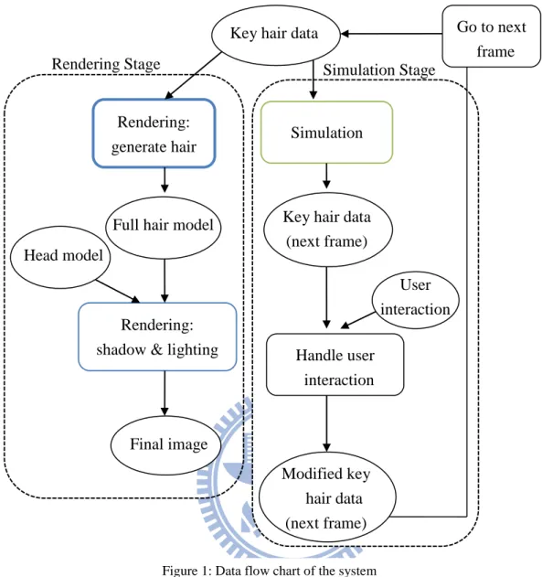
Figure 1: Data flow chart of the system ... 2
Figure 2: Input data of the system... 2
Figure 3: Control flow chart of the system ... 3
Figure 4: Rendering stage flow chart ... 7
Figure 5: Rendering pipeline of the B-spline tessellation step ... 8
Figure 6: Rendering pipeline of the single strand interpolation step ... 10
Figure 7: Rendering pipeline of the deep opacity maps generation step ... 11
Figure 8: Hair colored according to the layers. ... 12
Figure 9: The image of a deep opacity maps. ... 13
Figure 10: Rendering pipeline of the lighting and shadowing step ... 14
Figure 11: The procedure for advancing one time step of the system ... 15
Figure 12: The simulation flow chart ... 16
Figure 13: The distance constraint between two particles ... 17
Figure 14: Distance Constraints ... 18
Figure 15: Two sets of independent constraints ... 18
Figure 16: A scheme for solving distance constraints in one hair... 18
Figure 17: Pseudo code of the constraint solver kernel ... 19
Figure 18: Three sub-steps in the volume method step ... 20
Figure 19: A 2D MAC grid cell ... 21
Figure 20: A 3D MAC grid cell ... 21
Figure 21: Two example configurations of the markers ... 22
Figure 22: A 2D example of transferring the velocity of one particle ... 23
Figure 23: An example of transferring u ... 23
Figure 24: An example of transferring v ... 23
Figure 25: The VISITALLGRIDCELL procedure ... 24
Figure 26: The BUILDTRAVERSALDATA procedure ... 25
Figure 27: The VISITAGRIDCELL procedure ... 26
Figure 28: Configuration of the particles ... 27
Figure 29: An example of running the BUILDTRAVERSALDATA procedure ... 28
Figure 30: An example of running the VISITAGRIDCELL procedure ... 29
Figure 31: Pseudo code of making velocity field divergence free ... 30
Figure 32: Adding the difference of pressures to the u-component of velocity ... 31
Figure 33: The communication sequence of two threads in one frame ... 33
Figure 36: FPS versus viewing distance ... 38
Figure 37: Snapshots of the hair models in different level of details ... 38
Figure 38: Comparison between antialiasing turned off/on ... 39
Figure 39: Comparison between using/not using B-spline tessellation ... 39
Figure 40: Comparison between with/without interpolated hairs ... 40
Figure 41: Images of different numbers of interpolated hairs ... 40
Figure 42: Snapshots of hair with different directions of lighting ... 41
Figure 43: Images of hair with different colors ... 42
Figure 44: Two highlights of hair ... 42
Figure 45: Hair with different length changed at runtime ... 43
Figure 46: Snapshots taken in front of a character with long hair ... 44
Figure 47: Snapshots taken behind a character with long hair ... 45
Figure 48: Snapshots of real hair (part1) ... 46
Figure 49: Snapshots of real hair (part2) ... 47
Figure 50: An arbitrary small region of fluid ... 53
Figure 51: Tessellate control shader code of the B-spline tessellation step ... 56
Figure 52: Tessellate evaluation shader of the B-spline tessellation step ... 57
Figure 53: Tessellate control shader code of single strand interpolation step ... 58
List of Tables
Table 1: Comparison between using 1 and 3 kernels ... 31
Table 2: Number of grid cells versus FPS ... 36
Table 3: Number of grid cells versus number of PCG iterations ... 36
Table 4: Computation time percentage in one time step ... 37
Chapter 1: Introduction
1.1 Motivation
Hair animation has been seen in movies and games. Styling, rendering and simulation are the main issues in this topic. While in movie industry, the goal is to pursue film-quality image and a controllable dynamic behavior simulation. Computer games tend to find a balance between cost and performance, fulfilling the player‟s satisfaction and the running of games. For hair animation, we implement known algorithms on graphics hardware for real time hair rendering and simulation.
1.2 Overview
In this section, we describe the data flow of our system in a chart illustrated in Figure 1. The input of the system is a set of hair data called key hairs (shown in Figure 2) because extra hairs are generated from this set of hair for rendering. The input includes number of hairs, number of points per one hair strand, each point‟s position, velocity and mass and so on. In every frame, the key hair data go through the rendering stage and the simulation. The rendering stage includes two parts. The first part of the rendering stage generates a full hair model. The second part of the rendering stage takes the full hair model together with the head model to produce the final image. On the other hand, the simulation stage computes the key hair‟s position and velocity of the next frame. Then they are modified by handling the user input. Finally, the key hair data are updated when advancing to the next frame.
Figure 2: Input data of the system
We use two GPUs (Graphics Processing Unit) in this work. We use multithreading technique to coordinate two GPUs, one GPU runs the simulation code and other one runs the rendering code. There are two threads, one is the main thread and the other is
Rendering:
generate hair Simulation
Handle user interaction Rendering:
shadow & lighting
User interaction Key hair data
(next frame)
Modified key hair data (next frame) Full hair model
Final image
Key hair data
Head model
Rendering Stage Simulation Stage
Go to next frame
the worker thread. In each frame, the main thread first sends an event to activate the worker thread. And then, the two threads are run simultaneously. The main thread runs the rendering task on GPU One and the worker thread runs the simulation task on GPU Two. After both tasks are finished, the user interaction is handled. That is the end of the process of one frame. Then the system might go to next frame or exit the program. The control flow of the system we described is in the chart illustrated in Figure 3. Rendering (GPU 1) Simulation (GPU 2) Handle user interaction Activate the worker thread Start
Wait for both tasks (threads) to finish
Exit
Continue? Yes
No
1.3 Contribution
We presented a real-time rendering and simulation system based on graphics hardware. We follow the work by McAdams [4] to use a volume method borrowed from the field of fluid simulation. We present a realization of the steps of FLIP used in the hair simulation based on CUDA. We implement the staggered MAC (marker and cell) grid structure on the GPU. It allows the central difference to be accurate to O(∆x2) comparing with the work by Crane [16]. The preconditioned conjugate
gradient method is implemented on the GPU. It has a better convergence than the Jacobi iteration method in the problem we are dealing with.
We follow the work by Tariq [1] to use a tessellation based hair rendering scheme. Our implementation is based on the newly available tessellation stage in the rendering pipeline of OpenGL 4.0. We generate hairs for rendering from simulated key hairs dynamically using shaders on the GPU every frame. We achieve LOD (level-of-details) dynamically for rendering.
Chapter2: Related Works
We briefly review the previous works in hair simulation and hair rendering.2.1 Hair Simulation
Hair Strand Dynamics: There are different dynamic models for simulating the
motion of hair in the past researches. Rosenblum et al. modeled hair with mass-spring system [45] which was widely used in the field of cloth animation. Anjyo et al. modeled hair using projective dynamics [44]. Serial rigid multi-body chain was used to model strands such as hair, ropes or tails [42][39][25][18]. The technique was applied in the film “Shrek” and “Madagascar” by DreamWorks. Bertails et al. used the technique based on elastic rod theory and treated hairs as one-dimensional elastic objects [21]. The mass-spring model with augmented structure could capture more natural phenomena such as torsion [37][9].
Hair-hair Interaction: To capture the group motion of hair some techniques viewed
hair as a continuum and use fluid simulation based methods. Hadap used SPH (smoothed particle hydrodynamics) to model hair-hair, hair-air and hair-body interaction [42]. Bando et al. used loosely connected particles with SPH [36]. Petrovic et al. used a fixed grid volumetric method which was similar to an Eulerian fluid approach [23]. Bertails et al. used the hair-hair interaction force base on voxelized hair density [26]. Tariq and Bavoil handled hair-body and hair-hair interaction together by voxelizing obstacles in addition to hair [7]. McAdams et al. used a hybrid method in which a Lagrangian hair simulator and an Eulerian fluid solver were combined [4].
Some techniques simulate the collision and interaction on a sparse set of guide hairs to model the group behavior, such as [24][21][19][39]. In the rendering stage, more primitives are generated to produce a complete hair model. Chang et al. built additional triangle strips between two horizontal guide hairs for collisions to model the volume [39]. Plante et al. used a layered wisp approach which consisted of a skeleton curve, a deformable envelope and primitives for rendering [37][40]. Deformable lattice approach was used by [27][19].
Level-of-detail methods have been presented in [35][32][33]. Bertails et al. used an adaptive method that allowed guide hairs to split or merge [35]. The representation of hair was chosen based on visibility, viewing distance and hair motion in [32][33]. The LOD technique was adapted in the interactive modeling system of [12].
2.2 Hair Rendering
Hair Lighting Model: Kajiya and Kay presented a local scattering model to render
fur [46]. It became commonly used in the field of hair rendering. Marschner et al. conducted physically experiments and proposed a detailed scattering model [34]. The model had two reflection highlights and one transmission light. Scheuermann presented a real time implementation which modeled the two highlights in an art-directable fashion [28]. Nguyen and Donnelly presented a real time implementation using shaders [24]. It appeared in the demo by the Nvidia cooperation which showed off the capability of their graphics card. Neulander proposed an imaged based lighting technique for hair [29] and was used in the production of the movie “The Lion, the Witch and the Wardrobe” [17]. Zinke et al. presented a technique that approximated the multiple scattering of a full head of hair efficiently [5]. Ren et al. rendered hair with multiple scattering under environment lighting interactively [3]. Sodeghi introduced an approach that provided artist friendly controls over traditional physically based models [2]. It became part of the motion picture production pipeline and participated in the Disney film “Tangled”.
Hair Self-shadow: Hair casts shadow on itself and self-shadow is produced. Lokovic and Veach presented an off-line method called “deep shadow map” [43]. It computed the approximate light transmittance at all depth along the light-ray direction. Each pixel of the map was an approximate function. The technique could render hair with self-shadow. Kim and Neumann used a set of 2D maps to sample the opacity of hair along the light-ray direction and rendered hair with self-shadow efficiently [41]. The technique was called opacity maps and was used in the interactive editing and rendering system of [38]. Koster et al. presented a real time implementation of the opacity maps using graphics hardware using 3D textures [31]. Nguyen and Donnelly used the multi-render target feature of graphics hardware to generate 16 maps in one rendering pass [24]. Sintorn and Assarsson presented a quick-sort for lines using geometry shader on the GPU [8]. They generated 128 maps interactively using this method. Mertens et al. used k-means clustering algorithm to efficiently estimate the hair density along the light-ray [30]. Bertails used light-orient voxels to accumulate the transmittance in the hair volume [26]. Yuskel and Keyser pointed out that if the shape of the sampling map matches the shape of the hair, it could reduce the layering artifact of opacity maps efficiently [6].
Chapter3: Hair Rendering
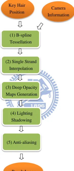
Figure 4: Rendering stage flow chart
In the rendering stage, there are five steps as illustrated in Figure 4. First, we generate nicer curves from the key hair in the B-spline tessellation pass. And then, we use the newly generated hair curves to perform single strand interpolation and produce more hairs. We generate the hair model on the GPU based on the work of [1].
Key Hair Position (1) B-spline Tessellation (2) Single Strand Interpolation (5) Anti-aliasing (4) Lighting Shadowing (3) Deep Opacity Maps Generation Camera Information Result Image
In step (3), the hairs are used to generate the shadow maps called deep opacity maps. Each light that casts shadow on the hair has its own set of deep opacity maps. Generating a set of deep opacity maps is a two-pass rendering process. We render the hair with lighting and shadows in step (4). Finally we perform the super-sampling antialiasing to compute the final image.
3.1 B-spline Tessellation
Figure 5: Rendering pipeline of the B-spline tessellation step
Vertex shader Key Hair position Tessellate control shader Tessellator Tessellate evaluation shader Geometry shader Transform feedback Tessellate level parameter Tessellated key hair position, hair
segment tangent vertex buffers
The rendering pipeline of the B-spline tessellation step is shown in Figure 5. The goal of this step is to generate a smooth hair curve from the original key hair. The key hair positions are stored as line strips in the vertex buffer. The number of vertices in a patch is set to four and the input indices are groups of four vertices. The vertex shader only passes down the data. The layout of the tessellate control shader is set to match the number of vertices in an input patch. The tessellate control shader takes a tessellate-level parameter and the tessellator generates primitives based on the parameter. It also computes the tangent of the segments and sends tangent data to tessellate evaluation shader as a per-patch constant data. The layout of the tessellate evaluation shader is set to isolines. It takes the parametric coordinate value as input to compute this vertex‟s position according to the uniform cubic B-spline formula. It also computes the tangent. The geometry shader does nothing but passes down the data. Then the tessellated vertices are sent back to vertex buffers (one for position and the other for tangent) via transform feedback. We list the tessellate control/evaluation shader code in Figure 51 and Figure 52 in Appendix C.
3.2 Single Strand Interpolation
The rendering pipeline of single strand interpolation step is shown in Figure 6. The goal of this step is to generate more hairs from the key hairs to produce a full hair model. The key hair position, the tangent along with each key hair‟s coordinate frame and a set of random uv-coordinate are bound to texture buffers. This allows random access to the key hair position and the tangent in the shaders. The drawing GL-API call invokes the pipeline to render without binding an actual vertex buffer. The vertex shader passes down the vertex-ID. The tessellate control shader outputs the tessellation-level indicating how many hairs are going to be interpolated from a key hair. The tessellate evaluation shader uses the vertex-ID to identify the segment in a hair and the key hair is it working. It fetches the corresponding vertex data and computes the interpolated vertex data. The geometry shader just passes down the primitive data. Then the hair positions and tangents are collected in two vertex buffers after transform feedback. We list the tessellate control/evaluation shader code in Figure 53 and Figure 54 in Appendix C.
Figure 6: Rendering pipeline of the single strand interpolation step
Tessellated key hair position,
tangent
Key hair tangent
Key hair position
Key hair coordinate frame
Texture buffer
A set of random uv coordinates Bind data to buffer Tessellate
level No vertex buffer input
Fetch from buffer
Interpolated hair position, tangent Vertex shader Tessellate control shader Tessellator Tessellate evaluation shader Geometry shader Transform feedback
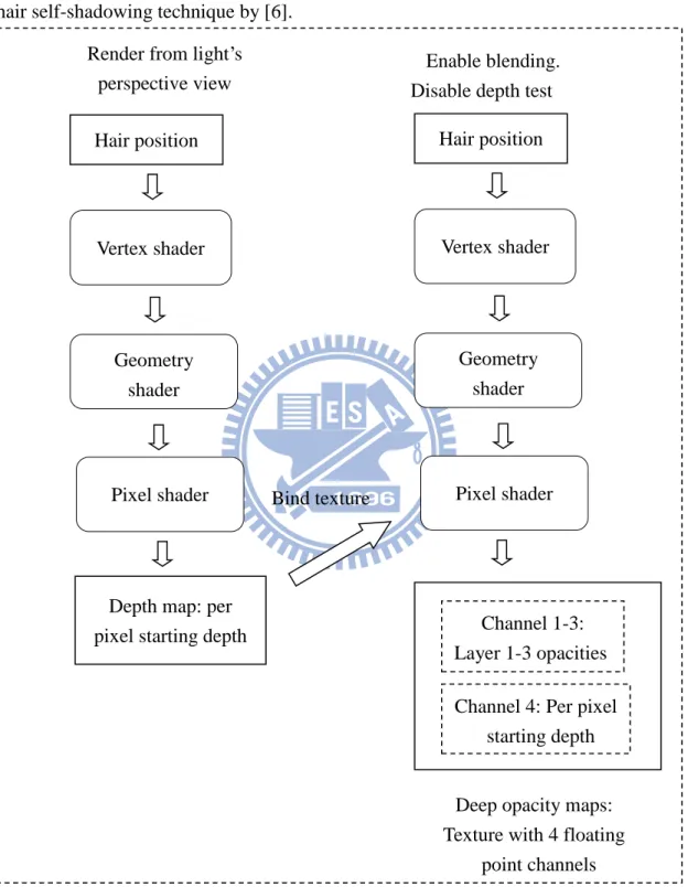
3.3 Generation of Deep Opacity Maps
The two-pass deep opacity maps generation is illustrated in Figure 7. This is the hair self-shadowing technique by [6].
Figure 7: Rendering pipeline of the deep opacity maps generation step
The first pass of generating the deep opacity maps is to render a depth map. Hair geometry is rendered from the light‟s perspective. A single channel floating point texture is used as the render target. Each pixel of the map is records the starting depth
Hair position
Channel 1-3: Layer 1-3 opacities Channel 4: Per pixel
starting depth Vertex shader
Geometry shader
Pixel shader
Depth map: per pixel starting depth
Enable blending. Disable depth test
Hair position Vertex shader Geometry shader Pixel shader Bind texture
Render from light‟s perspective view
Deep opacity maps: Texture with 4 floating
value of the hair geometry seen from the light. The vertex shader passes the view space depth value in addition to the clip space position. The geometry shader then passes down all the data. In the pixel shader, it writes out the depth in the view space. After all the hair geometry is rendered, the pixels record the starting depth value. The second pass accumulates the opacity of hair geometry and save the result to a texture. We choose to use three layers as it was shown effective enough in [6]. The distances between each layer are adjustable parameters. This pass is rendered with the blending enabled and the depth test disabled. The depth map generated from last pass is bound as the input texture. The vertex shader and geometry shader are the same as the first pass. The pixel shader computes the layer a pixel belongs to according to its depth value, the starting depth of hair geometry (fetched from the depth map texture) and the separation distances of the layers. A pixel contributes opacity to its layer and the layers behind. We store the accumulated opacities of the three layers in three channels of the texture (channel RGB). The depth map from the first pass is copied to the alpha channel (channel A). It allows us to access just one texture when using the deep opacity maps to compute the shadows.
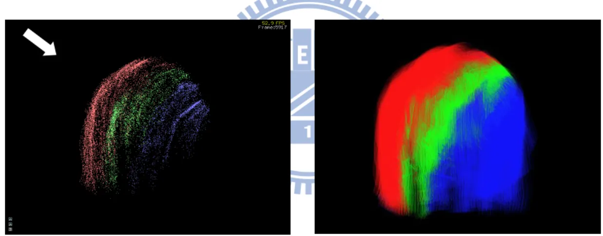
Figure 8: Hair colored according to the layers.
The left side of Figure 8 shows that the pixels in a layer of the deep opacity maps resemble the shape of hair geometry. The arrow indicates the direction of the light source. Pixels of each layer are marked with different colors. The shape of the red color pixels resemble the shape of hair geometry seen from the light‟s point of view. The second layer and third layer follow the shape of the first layer. The right side shows the hair colored according to the layers.
Figure 9: The image of a deep opacity maps.
The image of a deep opacity maps with RBG channels correspond to the accumulated opacities in the three layers is shown Figure 9. If a pixel is in the first layer, it contributes its opacity to all of the three layers. The RGB channels have the same value, so the color we see in the image is white. If a pixel is in the second layer, it contributes its opacity to the last two layers. The value of the R channel is zero and the GB channels have the value, so the color seen is cyan. If a pixel falls in the third layer, it contributes its opacity to the last layer. Only the B channel have nonzero value, so the color seen is blue.
3.4 Lighting and Shadowing
The pipeline of the lighting and shadowing step is shown in Figure 10. This step uses the vertex buffer generated from the interpolated steps to draw the hair geometry with lighting and shadowing. We proceed with the shading model used in [28] together with the deep opacity maps to compute shadows. As in [28] we fake the physically experimented hair scattering model by [34] by shifting the tangents to produce two specular highlights. We use two noise textures. One is used to break the strong highlights. And the other is a random noise to the tangent shift value. For each light that causes hair to cast self-shadow, we look up the deep opacity maps to compute shadows.
The vertex shader computes the clip space position, the view vector for lighting, the world space position and the tangent and the position in light‟s space for each light that induce hair self-shadow. The geometry shader passes down all the data to the pixel shader. The pixel shader does all the heavy work. It first shifts the tangent interpolated in the rasterize-stage. It computes the color according to the shading model for each light, then multiplies the color by the shadow value computed using the deep opacity maps.
Figure 10: Rendering pipeline of the lighting and shadowing step
3.5 Antialiasing
We use the super-sample antialiasing technique. We render the scene to an image twice the size of the displayed image. And then we take extra samples around the original location of the pixel and compute the average color value of the samples. And shrink the image to the size we want. In step (4), we render the scene to a texture. And in step (5) we use the texture as the input and in take five samples around the location of the pixel to compute the average color in the pixel shader to produce the final image.
Deep opacity maps Light 1, 2 Hair highlight
noise texture Texture
Hair tangent shift noise texture Hair vertex buffer
Parameters: light, hair Vertex shader Geometry shader Pixel shader
Chapter 4: Hair Simulation
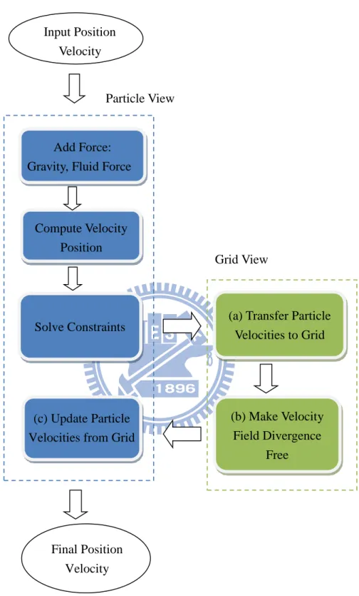
The simulation flow chart is shown in Figure 12. Our simulation approach is combined from the work by McAdams et al. [4] and Muller et al. [14]. We follow McAdams et al. [4] in using a volume technique from fluid simulation and follow the integration scheme and constraint formulation by Muller et al. [14].
In each time step, the input includes the position and velocity of the particles. We add external forces like gravity, fluid force or elastic spring force and compute the positions and velocities. We use elastic spring to model the force within a single hair [4]. These forces are adjustable and can be turned on or turned off. We require the system to meet some constraints (e.g. length constraint, angle constraint). The position and velocity are modified when solving the constraints iteratively. The next three steps are the sub-steps of the volume technique proposed by [4]. First, we transfer the velocities on the particles to the grid. Then we modify the grid velocities so that the divergence of the velocity field is zero. Making the velocity field divergence free is equivalent to making the fluid incompressible in fluid simulation. Finally we use the divergence-free velocity field on the grid to update velocities of the particles.
The procedure for advancing a time step of the system is outlined in Figure 11.
Figure 11: The procedure for advancing one time step of the system
The symbol 𝑣𝑖𝑛, 𝑥𝑖𝑛 is the velocity and position of the 𝑖𝑡ℎ particle at time 𝑡𝑛 and 𝑣𝑔𝑟𝑖𝑑𝑛 is the velocity on the grid structure which is explained in 4.2
1 Compute forces such as gravity
2 Compute velocity and position by applying the forces 𝑣𝑖𝑛 → 𝑣𝑖∗𝑛, 𝑥𝑖𝑛 → 𝑥𝑖∗𝑛 3 Solve constraint and modify position and velocity 𝑣𝑖∗𝑛 → 𝑣 𝑖𝑛, 𝑥𝑖∗𝑛 → 𝑥 𝑖𝑛 4 Proceed to the volume method step and modify the velocity
a) Transfer particle‟s velocity to the grid 𝑣 𝑖𝑛 → 𝑣𝑔𝑟𝑖𝑑𝑛
b) Make the grid‟s velocity field divergence free 𝑣𝑔𝑟𝑖𝑑𝑛 → 𝑣𝑔𝑟𝑖𝑑𝑛+1 c) Update particle‟s velocity from the grid velocity 𝑣𝑔𝑟𝑖𝑑𝑛+1 → 𝑣𝑖𝑛+1 5 Compute final position 𝑥 𝑖𝑛 → 𝑥𝑖𝑛+1
Figure 12: The simulation flow chart
Add Force: Gravity, Fluid Force
Compute Velocity Position Solve Constraints (b) Make Velocity Field Divergence Free
(a) Transfer Particle Velocities to Grid Grid View Particle View Input Position Velocity Final Position Velocity (c) Update Particle Velocities from Grid
4.1 Solving Constraints
We formulate and solve the constraints as in [14]. We employ the distance constraint for each segment of hair.
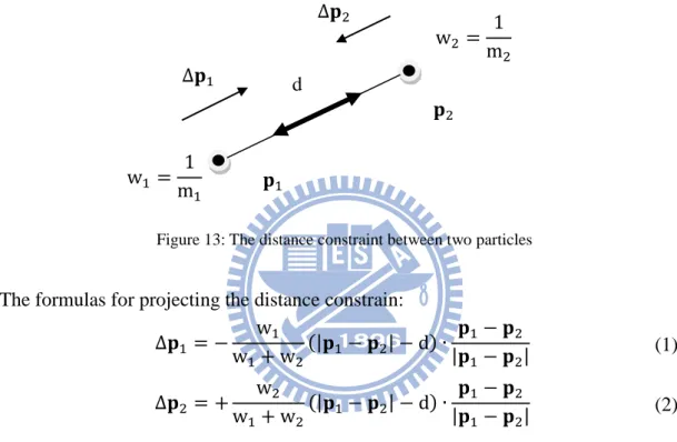
The case we are considering is illustrated in Figure 13. 𝐩1, 𝐩2 are the points of a
segment. w1, w2 are the inverse masses of the particles. The distance constraint
function is C(p1, p2) = |𝐩1− 𝐩2| − d. ∆𝐩1, ∆𝐩2 are the projection steps applied to
𝐩1, 𝐩2.
Figure 13: The distance constraint between two particles
The formulas for projecting the distance constrain: ∆𝐩1 = − w1 w1+ w2(|𝐩1− 𝐩2| − d) ∙ 𝐩1− 𝐩2 |𝐩1− 𝐩2| (1) ∆𝐩2 = + w2 w1+ w2(|𝐩1− 𝐩2| − d) ∙ 𝐩1− 𝐩2 |𝐩1− 𝐩2| (2)
Muller used Gauss-Seidal iterative constraint solver in [14]. Tariq implemented the solver using the geometry shader and the stream-out on DirectX 10 graphics cards and uses Direct Compute on cards supporting DirectX 11 in [1]. We follow the algorithm of [1] and implement on CUDA capable GPU. First we split the constraints into disjoint sets. Then we can project all the constraints in a set in parallel. The distance constraints can be separated into two sets. An example scenario is illustrated in Figure 14. In the figure, the circles represent the particle and the lines are the segments of hair. We generate a distance constraint for every segment. The two sets of constraints that can be projected in parallel (marked with bold lines) are illustrated in Figure 15.
∆𝐩1 ∆𝐩2 𝐩1 𝐩2 d w1 = 1 m1 w2 = 1 m2
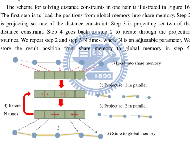
The scheme for solving distance constraints in one hair is illustrated in Figure 16. The first step is to load the positions from global memory into share memory. Step 2 is projecting set one of the distance constraint. Step 3 is projecting set two of the distance constraint. Step 4 goes back to step 2 to iterate through the projection routines. We repeat step 2 and step 3 N times, where N is an adjustable parameter. We store the result position from share memory to global memory in step 5.
1) Load into share memory
2) Project set 1 in parallel
3) Project set 2 in parallel 4) Iterate
N times
5) Store to global memory
Set 1 Set 2
Figure 15: Two sets of independent constraints Figure 14: Distance Constraints
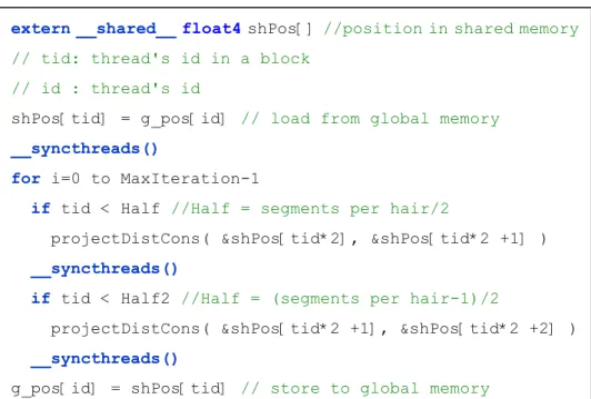
Figure 17: Pseudo code of the constraint solver kernel
The pseudo code of the constraint solver kernel is listed in Figure 17. We use one block of threads to solve the distance constraints of one hair. The number of threads per block is equal to the number of vertices per hair. The share memory size per block is equal to the number of segments per hair (number of distance constraints per hair) times the size of float4 (32*4 bytes). We pack the position (float3) and inverse mass (float) into the float4 data type.
Note that as stated in the CUDA programming guide [13], the __syncthread() is allowed in conditional statement only if the condition is evaluated the same by all the threads of an entire block. As a result, the __syncthread() instruction is placed outside the if-statement scope.
4.2 The Volume Method Step
There are sub-steps as we illustrated in Figure 18. We follow the approach of [4] and adapt the FLIP (fluid implicit particle) method of [22]. FLIP is a hybrid method using both particles and grid to simulate fluid. It was proposed by [47] and applied in graphics by [22]. It has the advantage of maintaining more details from being smoothened by numerical dispatching compared with an Eulerian approach (grid-based approach). In this chapter we introduce briefly the grid structure first and then explain the each of the sub-steps.
extern __shared__ float4 shPos[] //position in shared memory
// tid: thread's id in a block // id : thread's id
shPos[tid] = g_pos[id] // load from global memory
__syncthreads()
for i=0 to MaxIteration-1
if tid < Half //Half = segments per hair/2
projectDistCons( &shPos[tid*2], &shPos[tid*2 +1] ) __syncthreads()
if tid < Half2 //Half = (segments per hair-1)/2
projectDistCons( &shPos[tid*2 +1], &shPos[tid*2 +2] ) __syncthreads()
Figure 18: Three sub-steps in the volume method step
4.2.1 The Grid Structure in Fluid Simulation
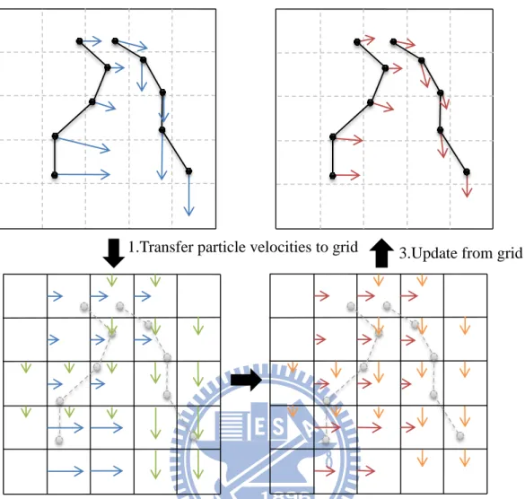
We use the staggered MAC (Marker and cell) grid structure. A two dimensional MAC grid is shown in Figure 19. We use the notation 𝑢⃗ = (𝑢, 𝑣) for the velocity, u is the component in x-direction and v is the component in y-direction. The notation ui+1/2,j is the u-component of the velocity stored at the center of grid cell face between cell (i, j) and (i+1, j). The notation vi,j+1/2 is the velocity‟s v-component located on the center of the grid cell face between cell (i, j) and (i, j+1). Notation Pi,j is the pressure at the center of grid cell (i, j). The velocities are stored on the grid cell faces and the pressures are stored at the centers. The u-components and the v-components of the velocities are stored at different faces. The blue squares mark the locations where u-components are stored and the orange squares mark the locations where v-components are stored. The blue and the orange arrows resemble u and v
2.Make the grid velocities field divergence free
3.Update from grid 1.Transfer particle velocities to grid
respectively. The red circles mark the locations where the pressure is stored.
Figure 19: A 2D MAC grid cell
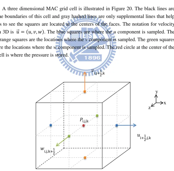
A three dimensional MAC grid cell is illustrated in Figure 20. The black lines are the boundaries of this cell and gray hashed lines are only supplemental lines that help us to see the squares are located at the centers of the faces. The notation for velocity in 3D is 𝑢⃗ = (𝑢, 𝑣, 𝑤). The blue squares are where the u component is sampled. The orange squares are the locations where the v component is sampled. The green squares are the locations where the w component is sampled. The red circle at the center of the cell is where the pressure is stored.
Figure 20: A 3D MAC grid cell
The meaning of the markers in a two dimensional MAC grid is shown in the left 𝑢i+1 2,j 𝑃i,j 𝑣i,j+1 2 y x 𝑃i−1,j 𝑃i,j−1 𝑣i,j−1 2 𝑢i−1 2,j 𝑢i+1 2,j,k 𝑃i,j,k 𝑤i,j,k+1 2 𝑣i,j+1 2,k z y x
side of Figure 21. The green dots are fluid particles. The cells containing any fluid particles are marked as fluid hence we see the capital „F‟ in blue square. The cells that are solid are marked as „S‟ and the cells that are air are marked as „A‟. In our application, the hair control points are the fluid particles as shown on the right side of Figure 21.
By using the staggered grid, we get a more accurate central difference. It is beneficial in the step of making fluid incompressible as mentioned in [20].
4.2.2 Transferring Particle Velocities to Grid
We explain the scenario of velocity transfer in the two dimensional case first. In Figure 22, the black grid is the staggered MAC grid. The black circle represents the position of a particle. The orange arrow is the particle‟s velocity vector u⃗ = (u, v) (u⃗ = (u, v, w) in 3D). We are going to transfer the u-component of the velocity onto the center of vertical grid faces and the v-component onto the center of horizontal grid faces. We transfer velocities to the center of faces within the distance of one grid cell size. We refer to the center of faces where the u-component is stored as the grid‟s u-faces and the center of faces where the v-component is stored as the grid‟s v-faces in the rest of the paragraphs. We draw blue squares on the four u-faces that have a nonzero transferred value and purple (magenta) squares on the four v-faces with nonzero transferred value.
Figure 22: A 2D example of transferring the velocity of one particle
The idea of transferring velocity u-component to the grid‟s u-faces is illustrated in Figure 23. The blue square resembles the u-faces. The arrows originated from the squares indicate the horizontal velocities on the u-faces.
In the following paragraphs, we describe how to traverse the particles in each grid cells parallelly. And we use this procedure to transfer the velocities on the particles to the grid. We follow the work of [Gre07] and modify their algorithm.
Algorithm overview: The procedure of visiting all the grid cells,
VISITALLGRIDCELL, is listed in Figure 25. After the arrays are initialized, we build the data used for the traversal in the BUILDTRAVERSALDATA procedure (line 13). Then we visit each of the cell parallely from line 16 to line 19.
The BUILDTRAVERSALDATA procedure is listed in Figure 26. We sort the data (position, velocity) of the particles by its grid cell id (line 17). The cell id of a particle is the id of the cell where this particle is located. Then the data of the particles in the same cell are placed together in the data arrays. We record the array index of the first particle of each cell in an array start_index from line 20 to line 25. If there is no
particle in a cell then the value of the array is the initial value Np, the number of particles.
The procedure of visiting a grid cell, VISITAGRIDCELL, is listed in Figure 27. This procedure takes the sorted data of the particles, position, velocity and cell id, and the lookup data start_index as input. We first get the array index of first particle by looking up in the start_index. Then we iterate through the particles in the for-loop (line 11). If the cell does not contain any particle, then the value of i_start is Np (the default value). In this case the termination condition of the for-loop is reached and the procedure ends. In the for-loop, there is another termination condition when the next cell id is different from the first id (line 15). It is because the data of the particles in a cell are placed together in the array. If the cell id is different from the first particle, then it means this particle belongs to anther cell. Consequently, the for-loop is exited.
Figure 25: The VISITALLGRIDCELL procedure 1 procedure VISITALLGRIDCELL(
2 in nx, ny, nz //are the number of grid cells in x, y, z dimensions 3 in Np // number of particles
4 in p[Np] // particle‟s position 5 in v[Np] // particle‟s velocity ) 6 begin
7 // initialization
8 Ncell = nx*ny*nz // total grid cells
9 sorted_cell_id new array [Np] // particle‟s cell id after sorting 10 start_index new array [Ncell]
11 p_sorted new array[Np], v_sorted new array[Np], 12 // build
13 BUILDTRAVERSALDATA ( Np, Ncell, p, v,
14 id_sorted, p_sorted, v_sorted, start_index) 15 // traversal
16 for each (i,j,k) 1<=i<nx-1, 1<=j<ny-1, 1<=k<nz-1 in parallel 17 compute cell id : id=i+nx*(j+ ny*k)
18 VISITAGRIDCELL ( id, Np, sorted_cell_id, 19 p_sorted, v_ sorted, start_index ) 20 end
Figure 26: The BUILDTRAVERSALDATA procedure 1 procedure BUILDTRAVERSALDATA ( 2 in Np // number of particles 3 in Ncell // number of cells 4 in p[Np] // particle‟s position 5 in v[Np] // particle‟s velocity
6 out sorted_cell_id [Np] // particle‟s cell id after sorting 7 out p_sorted [Np] //
8 out v_sorted [Np] // particle‟s velocity after sorting 9 out start_index [Ncell]
10 // starting particle‟s index in p_sorted, v_sorted array ) 11 begin
12 // initialization
13 for each i, 0<=i<Ncell in parallel 14 start_index[i] = Np
15 //sorting
16 compute particle‟s cell id by its position in parallel 17 sort particle‟s position and velocity by its cell id 18 output: p_sorted[], v_sorted[], sorted_cell_id[] 19
20 for each i, 0<=i<Np in parallel 21 if i!= 0 then
22 if sorted_cell_id[i-1]!= sorted_cell_id[i] then 23 start_index[sorted_cell_id[i]]=i
24 else
25 start_index[sorted_cell_id[i]]=0 26 end
Figure 27: The VISITAGRIDCELL procedure
We give a two dimensional example in Figure 28 and the configuration of the data structures is shown in Figure 29. The configuration of the particles is in shown in Figure 28. Each square represents a cell and the black number in each cell is the id of this cell. The blue circles represent the particles. The particles actually are volume-less in our model, but we draw the circles big enough for visualization. The white numbers in the circles are the id of the particles. For the computing the id of a cell, we use the following equation:
cell(i, j) id = i + 𝑛𝑥 ∙ j (3)
nx is the number of grid cells in the x dimension, which is 4 in this case.
We start running the VISITALLGRIDCELL procedure, after initialization (line 8-11), we step into the BUILDTRAVERSALDATA procedure.
In line 13-14 of BUILDTRAVERSALDATA, each element of the start_index array is initialized the number of total particles, Np, which is 6.
In line 16, the particle ids are computed. We show the idea in Figure 28. We find where the particles are and see the cell ids, which are the numbers labeled on the cells. For example, we see particle with label 0 is located at the cell label 9, so its cell id is 9.
1 procedure VISITAGRIDCELL ( 2 in id // cell id
3 in Np // number of particles
4 in sorted_cell_id [Np] // particle‟s cell id after sorting 5 in p_sorted [Np] //
6 in v_sorted [Np] // particle‟s velocity after sorting 7 in start_index [Ncell]
8 // starting particle‟s index in p_sorted, v_sorted array ) 9 begin
10 i_start = start_index[id] 11 for each i, i_start <= i < Np
12 //visit particle, its position, velocity are: 13 //p_sorted[ i ], v_sorted[ i ]
14 id_start = sorted_cell_id[ i_start ]
15 if i+1 >= Np || id_start != sorted_cell_id[ i+1 ] then 16 break // finish visiting all the particles in this cell 17 end
We sort the id of cells and id of the particles according to the id of cells. The cell ids of the particles before sorting and after sorting are shown in the 2nd and 3rd column in Figure 29. The particle data (position and velocity) before sorting and after sorting are shown in the 4th and 5th column in Figure 29.
In line 20-25 of BUILDTRAVERSALDATA, we fill data into the start_index array. When i=0, sorted_cell_id[0] is 4, then start_index[4] is 0.
When i=1, sorted_cell_id[0] == sorted_cell_id[1], nothing changed.
When i=2, sorted_cell_id[1] is 4 and sorted_cell_id[2] is 6, then start_index[6] is 2. When i=3, sorted_cell_id[2] == sorted_cell_id[3], nothing changed.
When i=4, sorted_cell_id[3] == sorted_cell_id[4], nothing changed.
When i=5, sorted_cell_id[4] is 6 and sorted_cell_id[5] is 9, then start_index[9] is 5. The result of star_index array is shown in the last column in Figure 29.
Figure 29: An example of running the BUILDTRAVERSALDATA procedure
We step out of the BUILDTRAVERSALDATA procedure and go to line 16 of VISITALLGRIDCELL. We visit all the cells in the parallel for-loop and step into VISITAGRIDCELL in line 18.
We choose the cell with id 6 as the example to show the VISITAGRIDCELL procedure. In line 10 of VISITAGRIDCELL, the i_start = start_index[ 6 ] is 2. Then the for-loop in line 11 becomes: for each i, 2 (i_start) <=i<6 (Np). The id_start is 6 When i=2, we visit particle with P1, V1. id_start is 6 and sorted_cell_id[3] is 6, the for-loop continues.
When i=3, we visit particle with P2, V2. id_start is 6 and sorted_cell_id[4] is 6, the for-loop continues.
When i=4, we visit particle with P4, V4. id_start is 6 and sorted_cell_id[5] is 9, the termination condition is reached and we exit the for-loop. Then the procedure ends. The above operation is shown in Figure 30. In the figure, the first arrow indicates that we get i_start by looking-up start_index[6]. The particle data that are visited is colored with blue. The second arrow indicates that we reach the termination coniditon of the for-loop when id_start (6) and sorted_cell_id[ i+1 ] (9) is different.
We run the VISITAGRIDCELL procedure with the cell with id 9 as another example. In line 10 of VISITAGRIDCELL, the i_start = start_index[ 9 ] is 5. Then the for-loop in line 11 becomes: for each i, 5(i_start) <=i<6 (Np). The id_start is 9
Let us choose the cell with id 7 (without any particle) and run the VISITAGRIDCELL procedure. In line 10 of VISITAGRIDCELL, the i_start = start_index[ 7 ] is 6. Then the for-loop in line 11 becomes: for each i, 6(i_start) <=i<6 (Np). After that the procedure ends.
We apply the VISITALLGRIDCELL procedure to transfer one of the velocity components. In the body of the parallel for loop (line 17-19), we visit all the neighboring cells instead of visit just one cell. The VISITAGRIDCELL procedure is modified to output the weighting and the weighted velocity component of the visited particle. And then the velocity outputs from the VISITAGRIDCELL are accumulated and stored to the grid.
The three components (u, v, w) of the 𝑢⃗ = (𝑢, 𝑣, 𝑤) are stored on the staggered structure. When we transfer u, we shift the origin of the grid by half a cell size along the y, z direction. So that the location of where u becomes the grid points. Similarly, we shift the origin of the grid along the x, z direction by half a cell size when transferring v. We run the modified VISITALLGRIDCELL procedure three times to transfer the velocity components u, v and w, respectively.
We store the data used for traversal on the texture memory for acceleration because of the uncoalesced memory access pattern.
4.2.3 Making Velocity Field Divergence Free
In this step, we are going to make the divergence of the velocity field on the grid become zero. We solve the linear system of pressure equations derived from the incompressible inviscid Navier-Stoke equations. Then we add the gradient of pressure to the grid velocities to satisfy the divergence free condition. We give a brief explanation of why making the velocity field divergence free preserves the incompressible feature of fluid in Appendix A. And a brief derivation of the pressure equation is given in Appendix B.
The pseudo code for this step is listed in Figure 31.
Figure 31: Pseudo code of making velocity field divergence free
In line 3, we compute the divergence of the velocity. In line 4, we formulate the matrix of the corresponding poisson system base on the [11] and [16]. In line 5, we compute the preconditioner required by the method. For the CPU version, we use the modified incomplete Cholesky and for the GPU version, we use the Jacobi preconditioner which is the diagonal of the original matrix.
In line 6, we solve the system of linear equation of pressure using the preconditioned conjugate gradient method as in [11]. In line 7 of Figure 31, we add the gradient of pressure to the velocities by:
u⃗ n+1= u⃗ n−∆t
ρ ∇p (4)
The case for adding the gradient of pressure to the u component is illustrated in Figure 32. We add the difference of the two red circles to the blue arrow in between when one of the two cells is fluid and neither one is solid. The operations for v and w component are carried out similarly.
1 void make_velocity_field_divergence_free() 2 {
3 compute_divergence(); //get r=div(u)
4 compute_poisson_coefficient(); //get matrix A
5 compute_preconditioner(); //preconditioner depends on A
6 solve_pressure(); //solve A p = r
7 add_pressure_gradient(); //u += grad(p)
Figure 32: Adding the difference of pressures to the u-component of velocity
When we implement this routine on the GPU, we put the cell marker and the pressure on texture memory for acceleration since the access pattern is not coalesced. We write a version which only uses one kernel function to do all the computation. We profile the routine using the CUDA profiler provided by Nvidia. There are many uncoalesced load of the global memory (access of u, w, and v). Then we write another version which splits the task into three kernel functions, each does the u, v, and w computation. And the profiler shows that the second version performs better than the first version, see Table 1. We presume the coalesced memory load/store save more time than the cost arisen by launching two more kernels.
Table 1: Comparison between using 1 and 3 kernels
add_pressure_gradient() implementation GPU time (usec) 1 kernel 17051 3 kernels 13255
4.2.4 Updating Particle Velocities from Grid
We update the velocities on the particles from the newly computed divergence free velocities on the grid. We follow the work of [4] and use the formula to update the velocity of the ith particle.
v i = α(vi+ Lerp(xi, vgrid− vgrid∗ )) + (1 − α)Lerp(x
i, vgrid), (5)
where Lerp(x, v) is the trilinear interpolation at the position x in the vector field v. vi
is the particle velocity before update, v i is the particle velocity after update and xi
is the particle position. vgrid is the divergence free grid velocities and vgrid∗ is the velocities before divergence free operation. 𝛼 is in the range [0, 1]. It is the parameter that controls the percent of FLIP and percent of PIC (particle in cell [48]) in the update. vi+ Lerp(xi, vgrid− vgrid∗ ) is the term for FLIP update and Lerp(xi, vgrid) is the term for PIC update. When α = 1, it is the pure FLIP update
and α = 0 is the pure PIC update. PIC has more numerical dissipation while FLIP is capable of producing detail but may develop noise.
𝑃i+1,j,k y x 𝑃i,j,k 𝑢i+1 2,j,k z 𝑢i+1 2,j,k+= ∆𝑡 𝜌 (𝑃i+1,j,k− 𝑃i,j,k) ∆x ∆x
For the implementation on the GPU, each thread loads the location of the particle and performs Lerp(x, v). We put both (vgrid− vgrid∗ ) and v
grid on the texture for
Chapter 5: Communication of Two
Threads
We use a threading mechanism for the coordination of two GPU. The communication sequence in each frame is shown in Figure 33.
Figure 33: The communication sequence of two threads in one frame
W ait W ait Start Event End Event Ack Event R un Rende r Code on GPU 1 R un S im ulation C ode on GPU 2 Set event Set event Return from wait
Set event Reset event Reset event Reset event Reset event Set event Return from wait
Return from wait
W
ait
Return from wait
W ait Main Thread Worker Thread
There are two threads in our scenario. One is the main thread and the other is the worker thread. There are three event objects. They are start-event, end-event, and ack-event (acknowledge-event). We create these event objects with the property of no automatic state reset. Consequently, we reset the state of the event object manually. The start-event is the event for the main thread to tell the worker thread to run its task in this frame. The end-event is for the main thread to tell the worker thread that this frame has finished and synchronize the result. The ack-event is for the worker thread to send an acknowledgement back to the main thread as a reply and let the main thread to reset the state of the event objects.
In the beginning of a frame, the worker thread is waiting for the start event. The main thread sets the start-event and waits for the ack-event from the worker thread. After the start-event is set, the worker thread returns from the wait state and sets the ack-event then start running the task of this frame. After it finishes the task, it waits for the end-event. After the ack-event is set, the main thread returns from the wait state and resets both the start-event and ack-event. Then it runs the task of this frame.
There are two possibilities at the end of the frame. One is that the main thread finishes its task first. The other is that the worker thread finishes its task first. In the first case, the main thread finishes its task. Then sets the end-event and waits for the ack-event from the worker thread. The worker thread has not finished yet, so the main thread remains in the wait state. When the worker thread finishes its task, it waits the end-event and returns from the wait state immediately. This is because the end-event has been set, then it sets the ack-event and goes to wait for the start-event in the next frame. Then the main-thread returns from the wait state when the ack-event is set. The main thread reset both the end-event and the ack-event and goes to the next frame. In the second case, the worker threads finishes first and waits for the end-event. It remains in the wait-state until the main thread finishes its task and sets the end-event. When this happens, the worker thread returns from the wait state and sets the ack-event then goes to the next frame. The main thread sets the end-event and waits for the ack-event. It immediately returns from the wait state since the ack-event has been set. Then it resets both the end-event and the wait-event and goes to the next frame.
We assign the main thread to run the rendering code and assign the worker thread to run the simulation code. Because CUDA context association is thread dependent, so all the thread dependent API calls must be called on the worker thread. So in the setup stage, we let the worker thread run the setup code first before going into the frame loop. The rendering API calls are performed on one graphics card and the simulation API calls falls on the other graphics card.
Chapter 6: Experiments and
Results
Hardware specification: The simulation code runs on a GPU with CUDA compute
capability 1.1 or above. The GPU we used was a Nvidia GeForce 9600GT. It was the middle-end consumer product of the GeForce 9000-GT series launched in Feb. 2008. It had 64 CUDA cores. Its graphics clock speed was 650 MHz and its memory bandwidth was 57.6 GB/sec. The rendering code requires a GPU that supports OpenGL 4.0 or above. We ran the rendering code on a Nvidia GeForce GTX480. It supported OpenGL 4.1. It was launched in March 2010. It had 480 CUDA cores. Its graphics clock speed was 700 MHz and its memory bandwidth was 177.4 GB/sec. The CPU we used was Intel i7-930. It was launched in the 1st quarter of 2010. It had 4 cores and 8 threads with clock speed 2.8 GHz.
Development environment: The operating system was Microsoft Windows XP
Professional with service pack 3. The GeForce driver installed was version 260.99. The development tool we used was Microsoft Visual Studio 2008. The Nvidia GPU Computing SDK version was 3.10. The BSGP compiler version was 2.0 by Huo [10].
Results: The snap shots from the motion of a character shaking her head are shown
in Figure 34. The number of key hairs, hairs rendered and primitives rendered were 1750, 28000 and 560000 respectively. There were three lights in the scene. Two sets of opacity maps were generated for the two spot lights which casted shadows. The number of simulated particles is 10500. The Flip grid is 32x32x32. The number of iteration of the constraint solver was 20.
Table 2: Number of grid cells versus FPS
Number of grid cells vs. FPS
163 323 643
CPU 21.8 13.3 3.19
GPU 96.2 86.5 37.7
Speedup 4.4x 6.5x 11.8x
The shows the performance comparison between the CPU and the GPU code is shown in Table 2. The performance was measured in FPS, frames per second. The result is also plotted in Figure 35. The speedup increased as the number of grid cell increased. The difference of the CPU and the GPU version of Flip was the preconditioner used in the precondition conjugate gradient (PCG) method. We chose the modified incomplete Cholesky (MIC) as [11] for the CPU code. We used the Jacobi preconditioner for the GPU code. We used the better preconditioner in the CPU code because some required computations were more difficult to realize on the GPU.
Figure 35: FPS versus number of grid cells between CPU and GPU version
Table 3: Number of grid cells versus number of PCG iterations
Number of grid cells vs.
number of PCG iterations
163 323 643
CPU 5.27 5.91 5.21
GPU 17.0 20.1 16.6
Table 3 shows the number of grid cells vs. number of PCG iterations of the GPU and CPU code. The tolerance for the PCG is 10−5. The preconditioner of the CPU
0 20 40 60 80 100 120 512 4096 32768 262144 FPS
Number of grid cells
CPU GPU
version makes the PCG to converged faster than the GPU version as shown by Table 3. The performance of the GPU version was better than the CPU version even though the preconditioner was inferior.
Table 4: Computation time percentage in one time step
The percentage of time spent in one time-step
CPU GPU
Solving constraints 31.4% 19.4%
Volume method 65.7% 76.6%
Compute force
velocity position 2.9% 4.0%
The computation time percentage is shown in Table 4. The most time consuming process is the volume step both in the GPU version and the CPU version. The time spent in the volume step in the GPU version is a higher because PCG took more iterations and the velocity transfer was more time consuming.
We used the viewing distance to adjust the number of hair segments generated in the rendering stage. When we viewed the hair model closely, we needed a detailed model. Whew we viewed the hair model from a far distance, we didn‟t need a detailed model and we used a coarse model. We used lesser segments when the camera was far and used more segments when the camera was near. This was the level-of-detail (LOD) method we used for rendering. Table 5 shows the FPS at different viewing distances with different screen resolution. The result is plotted in Figure 36. Because the number of pixel processed affected the rendering performance, therefore we measure FPS at different viewing distance with different screen resolutions. Figure 37 is the snapshots of the hair model adjusted for performance at different camera distances. We can observe that the FPS didn‟t increase when the viewing distance increased beyond a certain value. It was because the rendering task and the simulation task were run simultaneously in the process of one frame. Even if the render task was finish first, we had to wait until the simulation task finish to enter the next frame. When the simulation cost became higher than the rendering cost, the increase of rendering performance would not reflect on FPS anymore. And the simulation became the performance bottleneck.
Table 5: Viewing Distance versus FPS
Viewing distance vs. FPS 0.2 0.4 0.6 1.0 1.5 3.0 FPS (800x600) 25 44 63 98 136.1 136.1 FPS (1024x712) 20.6 40.2 59.6 93.2 136.1 136.1 FPS (1152x802) 18.3 36.9 56.1 88.7 136.1 136.1 FPS (1280x968) 15.9 31.9 50.9 83.2 136.1 136.1
Figure 36: FPS versus viewing distance
Figure 37: Snapshots of the hair models in different level of details
We used 2x super-sample antialiasing (SSAA) with a down-sampling filter pixel which takes five samples around a pixel. We show the comparison between the image with antialiasing turned off and the image with antialiasing turned on in Figure 38. The image with antialiasing turned off is shown in the left side of Figure 38 and the image with antialiasing turned on is shown in the right side of Figure 38. The image on right side has fewer jagged lines than the image on the left side and the down-sampling filter makes the lines looked thinner.
0 20 40 60 80 100 120 140 160 0 0.5 1 1.5 2 2.5 FPS Viewing Distance 800x600 1024x712 1152x802 1280x968
Figure 38: Comparison between antialiasing turned off/on
The comparison between the hair curves with B-spline tessellation and the hair curves without B-spline tessellation is shown in Figure 39. The hair curve with B-spline tessellation is shown in the left side of Figure 39 and the hair curve without B-spline tessellation is shown in the right side of Figure 39. The hair curves on the left side were smoother than the hair curves on the right side.
Figure 39: Comparison between using/not using B-spline tessellation
The comparison between the hair model with interpolated hairs and the hair model without interpolated hairs is shown in Figure 39. The hair model with interpolated hairs is shown in the left side of Figure 39 and the hair model without interpolated hairs is shown in the right side of Figure 39. The image on the left side has more hairs than the image on the right side.
Figure 40: Comparison between with/without interpolated hairs
The images of different numbers of interpolated hairs are shown in Figure 41. The original hair model is shown in the top left image. It had 1750 hairs. The number of hairs in the top right image was 4 times the number of hairs before interpolation (7000 hairs). The number of hairs in the bottom left image was 8 times the number of hairs before interpolation (14000 hairs). The number of hairs in the bottom right image was 16 times the number of hairs before interpolation (28000 hairs).
Figure 41: Images of different numbers of interpolated hairs
Images of hair with different lighting directions are shown in Figure 42. The lights were on the left side of the head in the top left image. The lights were in front of the head in the top right image. The lights were on the right side of the head in the bottom left image. The lights were behind the head in the bottom right image.
Figure 42: Snapshots of hair with different directions of lighting View direction Light direction View direction Front Back Light direction Head Back Head Front Back Head Front Head
Images of hair with different hair colors are shown in Figure 43. The hair was brown in leftmost image. The hair was black in the middle image. The hair was yellow in the rightmost image.
Figure 43: Images of hair with different colors
We shifted the tangents to produce two highlights. There was one white highlight and one dark-brown highlight on the hair shown in Figure 44.
Figure 44: Two highlights of hair
We could reset the constraints of hair to change the length of hair at runtime. We didn‟t change the length of segments near the hair root. We only changed the segment near the tip of the hair. The hairs were set shorter on the left side and the hairs were set longer on the right side as shown in Figure 45.
Figure 45: Hair with different length changed at runtime
We animated a character with long hair shaking her head. The snapshots taken in front of the character are shown in Figure 46. The snapshots taken behind the character are shown in Figure 47.
Figure 46: Snapshots taken in front of a character with long hair
(5)
(1) (2)
Figure 47: Snapshots taken behind a character with long hair
Because the goal of computer animation is to imitate the real world, we compare the hair animated by the computer program with the hair in the real world. The snapshots of the real hair are shown in Figure 48 (part 1) and Figure 49 (part 2).
The highlight of the hair from the real world video glistened more smoothly and brightly than the computer animated highlight. And the majority of the real hairs moved as a whole group while the computer animated hairs seemed to be moving more independently.
(5)
(1) (2)