氣膠微粒在管流中熱泳附著之研究

國 立 交 通 大 學

環境工程研究所

博 士 論 文

氣膠微粒在管流中熱泳附著之研究

THERMOPHORETIC DEPOSITION OF AEROSOL

PARTICLES

IN TUBE FLOW

研 究 生 ：林智賢

指導教授 ：蔡春進

氣膠微粒在管流中熱泳附著之研究

THERMOPHORETIC DEPOSITION OF AEROSOL PARTICLES

IN TUBE FLOW

研 究 生 ：林智賢 Student: Jyh-Shyan Lin

指導教授 ：蔡春進 Advisor: Chuen-Jinn Tsai

國立交通大學

環境工程研究所

博士論文

A Dissertation

Submitted to Institute of Environmental Engineering

College of Engineering

National Chiao Tung University

in Partial Fulfillment of the Requirements

for the Degree of

Doctor of Philosophy

in

Environmental Engineering

July, 2004

Hsinchu, Taiwan, Republic of China

摘要

本研究探討管流中微粒的熱泳附著效率。當流場與溫度場皆是在發展狀態 時，溫度梯度在圓管進口附近靠近管壁的位置是最高的，微粒的熱泳附著效率可 能會增加。因此，本研究首先利用數值模擬的方法探討進口流效應對圓管中微粒 熱泳附著效率的影響。而由於 Romay 等人(1998)的紊流熱泳附著效率的實驗值 與理論值不合，所以本研究接著用實驗的方法，探討微粒在圓管中的熱泳附著效 率並與理論值比對。最後，工業上常用管壁加溫的方法來防止微粒的管壁附著， 但是有效防止微粒附著的加熱溫度並未知，因此本研究利用數值模擬及實驗的方 法探討微粒在層流圓管中的附著效率。 在發展中的流體對微粒熱泳附著效率影響的研究中，以數值方法來求取微粒 在圓管中的臨界軌跡線，藉以計算出對應的熱泳附著效率。研究結果顯示，當流 場是完全發展流而溫度場是正在發展中的狀態，微粒的熱泳附著效率只有在圓管 進口的位置會稍微高於前述當流場與溫度場皆是完全發展流的案例，然而在Z>5 的圓管中，最終的熱泳附著效率會一樣。當流場與溫度場皆是正在發展中的情況 時，在 Z>5 的圓管中，微粒的熱泳附著效率大約是流場與溫度場皆是完全發展 流案例的兩倍，而且在進口的位置附著效率會高出甚多。另外，本研究開發出可 用在計算層流圓管中，流場與溫度場同時是完全發展流或同時是正在發展中的熱 泳附著效率半經驗式。 在層流及紊流圓管的微粒熱泳附著效率實驗中，本研究使用單徑的氯化鈉微 粒(微粒粒徑在 0.038 到 0.498 µm 之間)作為測試微粒，用來量測在一長 1.18 公 尺，內徑為0.43 公分圓管中微粒的熱泳附著效率。在 Romay 等人(1998)的研究 中，理論的熱泳附著效率和實驗值不合，然而在本研究中，考慮帶有Boltzmann

靜電平衡微粒的靜電附著、微粒的紊流擴散及慣性衝擊等機制，所以微粒的熱泳 附著效率可以準確地被量測出來。 在使用熱泳力來抑制微粒管壁附著這方面，我們將管壁加高溫度使其高於進 氣氣流，係利用實驗及數值模擬的方法探討微粒在層流圓管內的附著效率。在數 值分析這方面，求解包含熱泳項的對流擴散方程式，求得微粒在圓管內的濃度分 佈及附著效率。實驗時使用單徑微粒(微粒粒徑為 0.01, 0.02 and 0.04 µm)作為測 試氣膠，量得的實驗值用來驗證數值解。研究結果顯示，微粒的附著效率會隨著 管壁溫度的升高或是圓管內氣流量的增加而降低。本研究發展出一個半經驗式可 以用來預測在層流圓管中，在給定的無因次附著參數下，求得所需要的無因次溫 度差(亦即可求取所需的管壁加熱溫度)來達到零微粒附著效率。

ABSTRACT

This study investigates thermophoretic particle deposition efficiency in a tube flow. The highest temperature gradient near the wall occurs at the entrance of a tube when both flow and temperature are developing, thermophoretic deposition in the entrance region may be enhanced. Therefore, the effect of entrance flow on the thermophoretic deposition efficiency in laminar tube flow was first investigated numerically. In the previous study of Romay et al. (1998), the experimental data don’t agree well with theoretical results. In the present study, the thermophoretic particle deposition efficiency in tube flow was studied experimentally and compared with the theoretical predictions. To prevent particle deposition on tube wall, a common practice is to heat up the tube wall in industry. But the required wall temperature to effectively suppress particle deposition in tube wall is unknown. Thus the effect of tube wall temperature on particle deposition efficiency under laminar flow condition was investigated experimentally and numerically.

In the study of developing flow effect in a circular tube on thermophoretic particle deposition efficiency, the critical trajectory method was investigated numerically. The results show that when the flow is fully developed and temperature is developing, it is found that only near the thermal entrance region (or temperature jump region) of the tube the deposition efficiency is slightly higher than the combined fully developed case (flow and temperature), while the deposition efficiency remains the same for Z>5. When both flow and temperature are developing (or combined developing), the deposition efficiency is about twice of the combined fully developed case for Z>5 and is much higher near the entrance of the tube. Non-dimensional equations are developed empirically to predict the thermophoretic deposition

efficiency in combined developing and combined fully developed cases under laminar flow condition.

In the experimental study of thermophoretic deposition of aerosols particles in laminar and turbulent tube flow. Thermophoretic deposition of aerosols particles (particle diameter ranges from 0.038 to 0.498 µm) was measured in a tube (1.18 m long, 0.43 cm inner diameter, stainless-steel tube) using monodisperse NaCl test particles under laminar and turbulent flow conditions. In the previous study by Romay et al. (1998), theoretical thermophretic deposition efficiencies in turbulent flow regime do not agree well with the experimental data. In this study, particle deposition efficiencies due to other deposition mechanisms such as electrostatic deposition for particles in Boltzmann charge equilibrium, and turbulent diffusion and inertial deposition were carefully assessed so that the deposition due to thermophoresis alone could be measured accurately.

In the aspect of suppression of particle deposition by thermophoretic force, flow through a tube with circular cross section was investigated numerically and experimentally for the case when the wall temperature exceeds that of the gas. Particle transport equations for convection, diffusion and thermophoresis were solved numerically to obtain particle concentration profiles and deposition efficiencies. The numerical results were validated by particle deposition efficiency measurements with monodisperse particles (particle sizes were 0.01, 0.02 and 0.04 µm). For all particle sizes, the particle deposition efficiency was found to decrease with increasing tube wall temperature and gas flow rate. An empirical expression has been developed to predict the dimensionless temperature difference needed for zero deposition efficiency in a laminar tube flow for a given dimensionless deposition parameter.

誌謝

感謝指導教授 蔡春進教授在論文研究期間的殷情指導，使本論文得以完 成。特別感謝中央大學 李崇德教授、中興大學 鄭曼婷教授、交通大學 葉弘德 教授、白曛綾教授及元智大學 張幼珍教授的指導與協助定稿，使本論文更臻理 想。 在研究過程中，實驗室的學弟晉儀、林宏、力群、妮芬、世勳、士軒、開亨、 茂銓、思敏、正生、依馨、健倫及已畢業的學弟妹的彼此勉勵與幫忙，使得研究 生活多采多姿。由衷的感謝 江漢全教授，謝謝您在我求學過程中給予最大的協 助與幫忙。感謝 張振平博士在論文初期給予的協助。好友世興學長、裕強學長、 誌仁、凱文及高中的同窗好友們，謝謝您們在我讀博士期間的加油與精神上的支 持。另外，感謝在論文研究期間，當我遇到挫折時鼓勵及幫助我的所有長輩及朋 友，謝謝您們。 最後，僅以本文獻予敬愛的爸媽，感謝你們雖然已漸漸年老，仍給予我最大 的支持與鼓勵，姐文琪、妹淑華、弟智偉及女友家宜，有了你們一起生活及互相 扶持，使我能安心的完成學業，在此將論文獻於您們。

TABLE OF CONTENTS

Abstract (Chinese) I

Abstract (English) III

Acknowledgments V Table of contents VI List of tables IX List of figures X Nomenclature XIII Chapter 1 Introduction 1

1.1 Thermophoretic coefficient and thermophoretic velocity 1 1.2 Thermophoretic deposition efficiency in laminar tube flow 3 1.3 Thermophoretic deposition efficiency in turbulent tube flow 8 1.4 Isothermal particle deposition mechanisms in tube flow 10 1.5 Application of thermophoretic force to suppress particle deposition 15

1.6 Objectives of this study 17

Chapter 2 Numerical methods 18

2.1 Temperature field 18

2.2 Critical particle trajectory method to calculate thermophoretic particle

deposition efficiency 22

2.3 Solutions of convection-diffusion equation to obtain thermophoretic

particle deposition efficiency 28

Chapter 3 Experimental methods 30

3.1 Aerosol generation and conditioning 30

3.3 Experimental procedure 34

Chapter 4 Entrance effect on the thermophoretic deposition efficiency 38 4.1 Thermophoretic deposition efficiency for fully developed temperature and

velocity fields 38

4.2 Thermophoretic deposition efficiency for fully developed flow and

developing temperature 41

4.3 Thermophoretic deposition efficiency for developing flow and developing

temperature 42 4.4 Empirical equation of thermophoretic deposition efficiency for the case of

a long tube 48

Chapter 5 Experimental results of the thermophoretic deposition efficiency 51 5.1 Particle deposition efficiency due to isothermal deposition mechanisms 51

5.2 Thermophoretic deposition efficiency 56

Chapter 6 Suppression of particle deposition by thermophoresis 61 6.1 Thermophoretic deposition efficiency for tube wall temperature lower than

that of gas flow 61

6.2 Effect of temperature difference between the tube and gas flow on the

particle deposition efficiency 64

6.3 Particle deposition efficiency versus dimensionless temperature difference

and deposition parameter 67

6.4 An equation to predict the dimensionless temperature difference needed for

zero particle deposition 75

6.5 Practical application 76

Chapter 7 Conclusions and future study 77

7.2 Future study 79

Appendix A 81

References 83 Vita 89

LIST OF TABLES

Table 1.1 Theoretical expressions of thermophoretic deposition efficiency for a long tube where the temperature of hot gas has approached that of the wall. 6 Table 1.2 The values of φ0 at different PrKth and θ* for the short tube case. 6

Table 1.3 The exact solution of Walker et al. (1979) for thermophoretic deposition

efficiency in the long tube case. 7

Table 1.4 Theoretical expressions of the thermophoretic deposition efficiency in

turbulent tube flow. 9

Table 3.1 Experimental conditions of deposition measurement. 36 Table 3.2 Experimental conditions of suppression measurement. 37 Table 4.1 Accumulated thermophoretic deposition efficiency of combined

developing case and combined fully developed case at different positions

LIST OF FIGURES

Figure 1.1 Fluid element. 9

Figure 2.1 The developing velocity profiles in laminar tube flow. 23 Figure 2.2 Comparison between Graetz’s solution and temperature profile in the

thermal entry region with that of Grigull and Tratz (1965). 24

Figure 2.3 Critical particle trajectory. 25

Figure 3.1 The schematic diagram of the experimental setup for deposition

experiment. 31 Figure 3.2 The schematic diagram of the experimental setup for suppression

experiment. 32 Figure 4.1 Comparison of theoretical deposition efficiency with previous theories in

laminar tube flow. 39

Figure 4.2 Comparison of present theoretical thermophoretic deposition efficiency with numerical prediction of Stratmann et al. (1994) in laminar tube flow.

40 Figure 4.3 Comparison of accumulated thermophoretic deposition efficiency between

different θ*_{s versus Z, fully developed flow. 43}

Figure 4.4 Dimensionless temperature profiles as a function of dimensionless radial

and axial coordinates. 44

Figure 4.5 Accumulated thermophoretic deposition efficiency of aerosol particles using different numbers of grids, combined developing case. 45 Figure 4.6 Comparison of accumulated thermophoretic deposition efficiency between

different θ*_{s versus Z. 46}

Figure 4.7 Thermophoretic deposition efficiency as a function of thermophoretic parameter β1 in laminar fully developed flow and developing flow. 50

Figure 5.1 Comparison of experimental deposition efficiencies (isothermal) and theoretical predictions of diffusional and electrostatic deposition under

laminar flow conditions, (Re = 1340). 52

Figure 5.2 Comparison of experimental deposition efficiencies (isothermal) and theoretical predictions of combined turbulent diffusion and inertial deposition under turbulent flow conditions (Re = 6580). 54 Figure 5.3 Comparison of experimental data and theoretical predictions of

thermophoretic deposition efficiency of combined fully developed case under laminar flow conditions. (a) Re = 1340, Te = 343 K (b) Re = 1340,

Te = 373 K. 55

Figure 5.4 Comparison of experimental data and theoretical predictions of thermophoretic deposition efficiency of Romay et al. (1998) under turbulent flow conditions. (a) Re = 6580, Te = 343K (b) Re = 10200, Te =

343K. (c) Re = 10200, Te = 398K. 58

Figure 5.5 Comparison of theoretical predictions (Re = 10200) for particles of 0.05 and 0.498 µm in diameter in turbulent flow. 59 Figure 5.6 Comparison of experimental thermophoretic coefficients Kth with theories.

Experimental Kth is calculated based on experimental data and theoretical

thermophoretic deposition efficiency in (a) laminar flow (b) turbulent flow.

60 Figure 6.1 Particle deposition efficiency as a function of dimensionless parameter,

µ’=πDL/Q, for isothermal case. 62

Figure 6.2 Dimensionless temperature profiles as a function of dimensionless radial

Figure 6.3 Particle deposition efficiency versus tube wall temperature for NaCl particles with particle diameter of (a) 0.01 µm (b) 0.02 µm (c) 0.04 µm. The test tube length and inner diameter are 1.18 and 0.0043 m, respectively, and the inlet air temperature is 296 K. 65 Figure 6.4 Particle deposition efficiency as a function of the dimensionless

temperature difference, Tw/(PrKth(Tw-Te)), and deposition parameter,

πDL/Q. Dimensionless deposition parameter is (a) from 1.6×10-4 _to

1.2×10-2 _{and (b) from 1.2×10}-2 _{to 1.16. (Insets in the figures are}

deposition efficiency curves near zero deposition efficiency. For air and current tube geometry and length, the corresponding wall temperature is

marked in the upper x-axis). 70

Figure 6.5 The variation of radial particle thermophoretic and diffusional velocities in the axial direction as the tube wall is heated at various temperatures at a given particle diameter of (a) 0.02 µm (b) 0.005 µm and a constant flow

rate of 1 l min-1. 71

Figure 6.6 (a) Dimensionless radial concentration profiles and (b) dimensionless radial temperature profiles as a function of dimensionless axial coordinates. The test tube length and inside diameter are 1.18 and 0.0043 m,

respectively. 72 Figure 6.7 The relationship between the required dimensionless temperature

difference, θ = Tw/(PrKth(Tw-Te)), and the dimensionless deposition

parameter, µ’ = πDL/Q, for zero particle deposition for a circular tube air flow. Symbols represent the numerical results and solid line is the fitted

NOMENCLATURE

B dynamic mobility B = C/3πµ’dp [m N-1 s-1]

cp specific heat capacity at constant pressure [kj kg-1 K-1]

C slip correction factor [-] Cd drag coefficient [-]

Cm momentum exchange coefficient [-]

Cs thermal slip coefficient [-]

Ct temperature jump coefficient [-]

dp diameter of the particles [m]

D particle diffusivity [m2 s-1] Dt tube diameter [m]

e elementary unit of charge [C] f fanning friction factor [-]

h convective heat transfer coefficient [W m-2 _K-1_]

kg gas thermal conductivity [W m-1 K-1]

kp particle thermal conductivity [W m-1 K-1]

K Boltzmann constant [N m K-1] KE a constant of proportionality [N m2 C-2] Kth thermophoretic coefficient [-] L tube length [m] mp particle mass [kg] np particle charge [-]

N particle number concentration [1 m-3]

Pd, particle penetration efficiency [-]

Pd, A diffusional penetration efficiency in laminar tube flow [-]

Peg gas Peclet number (um⋅r02)/(α⋅L) [-]

Pr gas Prandtl number [-]

Ptur inertial impaction efficiency in turbulent tube flow [-]

q the charge on the particle [-] Q inlet gas flow rate [m3 s-1] r radial coordinate [-] r0 tube radius [m]

rc critical radial position [m]

R dimensionless radial coordinate r/r0 [-]

Rc dimensionless critical radial position rc/r0 [-]

Re Reynolds number [-]

Rep particle Reynolds number [-]

Sc Schmidt number [-]

t the elapsed time in the tube [s]

T average temperature of the fluid [K]

T gas temperature [K]

Te gas temperature at tube inlet [K]

Tm mixing-cup temperature [K]

Tw wall temperature [K]

T∞ free stream temperature [K]

T

∇K temperature gradient [K m-1] u gas velocity (z-component) [m s-1]

u* _{friction velocity}

2

* f

u

u = _m [m s-1]

um average gas velocity [m s-1]

v gas velocity (r-component) [m s-1] Vd particle deposition velocity [m s-1]

th

VK thermophoretic velocity [m s-1]

z axial coordinate [-]

z+ dimensionless axial coordinate z/(r0RePr) [-]

zdep thermal entrance length [m]

Z dimensionless distance from the entry Z = z/(0.05DtPeg) [-]

Greek letters

α thermal diffusivity kg/(ρ⋅Cp) [m2 s-1]

β1 thermophoretic parameter (in laminar tube flow) β1 = PrKth/(Te-Tw)/Tw [-]

δdf dust free layer [m]

ε0 the permittivity of air [C2 N-1 m-2]

η thermophoretic deposition efficiency [-] ηe electrostatic deposition efficiency [-]

η_A isothermal particle deposition efficiency in laminar tube flow [-] η_Am thermophoretic deposition efficiency in laminar tube flow [-]

ηt isothermal particle deposition efficiency in turbulent tube flow [-]

ηtur thermophoretic deposition efficiency in turbulent tube flow [-]

λ mean free path of air [m] µ air dynamic viscosity [N s m-2]

v _{air kinematic viscosity [N s m}-2_]

θ dimensionless temperature difference [-] θ* _{dimensionless temperature T}

w/(Te-Tw) [-]

ρg gas density [kg m-3]

ρp particle density [kg m-3]

τ particle relation time τ = ρpdp2C/18µ’ [s]

τ+ _{dimensionless particle relation time τ}+ _{= u}*2_/

CHAPTER 1

INTRODUCTION

Thermophoresis is a physical phenomenon that aerosol particles move toward the direction of decreasing temperature when subjected to a thermal gradient. Knowledge of thermophoresis is of great interest as it has various industrial applications. Extensive experimental and theoretical works have been published on thermophoretic coefficient (Waldmann, 1961; Brock, 1962; Derjaguin et al., 1976; Talbot et al., 1980), thermophoretic particle deposition efficiency in laminar duct and channel flow (Walker et al., 1979; Stratmann et al., 1994; Tsai and Lu, 1995), thermophoretic particle deposition efficiency in turbulent duct and channel flow (Nishio et al., 1974; Romay et al., 1998; He and Ahmadi, 1998). In industrial applications, thermophortic force has been used to enhance particle deposition efficiency on impactor substrate (Lee and Kim, 2002); to suppress particles deposition on wafer surface (Stratmann and Fissan, 1988); to design a particle control device for diesel engine exhaust (Messerer et al., 2003).

In this chapter, literature related to thermophoretic coefficient and thermophoretic velocity, thermophoretic deposition in laminar and turbulent tube flow, isothermal deposition mechanisms in tube flow and the application of thermophoretic force to suppress particle deposition is reviewed first. The motivation of this study is also explained, followed by the objectives of this study.

1.1 Thermophoretic coefficient and thermophoretic velocity

(Brock, 1962; Derjaguin et al., 1976; Talbot et al., 1980). The thermophoretic velocity can be calculated as

T T K V th th =− ∇ K K _ν (1.1)

where Kth is the thermophoretic coefficient derived by Derjaguin et al. (1976) as

⎟ ⎟ ⎠ ⎞ ⎜ ⎜ ⎝ ⎛ + + + = ) / 2 ( 2 ) / ( 2 1 ) / 2 ( / 2 . 2 p t p g p t p g th d C k k d C k k K λ λ ν (1.2)

The experimental results of Derjaguin et al. (1976) show good agreement with their own theory, but deviate from those of Talbot et al. (1980) who derived the expression for thermophoretic coefficient as

⎟ ⎟ ⎠ ⎞ ⎜ ⎜ ⎝ ⎛ + + + × + = ) / 2 ( 2 ) / ( 2 1 ) / 2 ( / )) / 2 ( 3 1 ( 2 p t p g p t p g p m s th d C k k d C k k d C C C K λ λ λ ν (1.3)

This formula approaches the Waldmann’s free molecular formula (1961) when Kn>>1 and the continuum-regime theory of Brock (1962) when Kn ≤ 0.2. Talbot et al. (1980) had given evidence that their expression is accurate for all regimes from free molecular to continuum flow. The thermophoretic coefficient of Talbot et al. (1980) is most widely used to calculate thermophoretic deposition efficiency in duct and channel flow, such as in Batchelor and Shen (1985), Ye at al. (1991a), Montassier et al. (1991), Stratmann et al. (1994) and He and Ahmadi (1998).

Chang et al. (1995) has investigated thermophoretic deposition in an annular flow with fixed thermal gradients between two cylinders experimentally and numerically. The implicit finite difference method was applied to solve particle transport equation due to convection, diffusion and thermophoresis when assuming fully developed flow. They found that the experimental thermophoretic deposition efficiency is generally closer to the numerical prediction using the thermophoretic coefficient of Derjaguin et al. (1976), as compared to that using thermophoreic coefficient of Talbot et al. (1980). However, the difference between the predicted deposition efficiencies obtained from the two models is too small in comparison with the magnitude of fluctuation in the aerosol source. As a result, Chang et al. (1995) stated that it is impossible to conclude which theory is more accurate.

Tsai and Lu (1995) designed a plate-to-plate thermal precipitator using forced convection heat transfer arrangement to enhance thermophoretic particle collection efficiency. They found that the thermophoretic coefficient proposed by Talbot et al. (1980) fits very well with their experimental data.

1.2 Thermophoretic deposition efficiency in laminar tube flow

Previous theories on thermophoretic deposition efficiency in laminar tube flow, listed in Table 1.1, are restricted to fully developed flow only. These equations are applicable for a long tube where gas temperature approaches that of the wall. In previous theories, Walker et al. (1979) and Batchelor and Shen (1985) considered particle transport due to convection and thermophoresis only, thermal diffusivity of particle was neglected. Such assumption is valid only when the dimensionless

deposition parameter for laminar diffusion, ε (ε =D L/Q), is much less than

0.0001 (Hinds, 1999). Walker et al. (1979) developed two models, one for a short tube, and another for a sufficiently long tube where gas temperature approaches that of the tube wall. For the short tube, Walker et al. (1979) solved the particle transport equation analytically and developed the following equation for thermophoretic deposition efficiency: 0 3 / 2 * Pr 07 . 4 φ θ η _⎟⎟ ⎠ ⎞ ⎜ ⎜ ⎝ ⎛ = g th Pe z K (1.4)

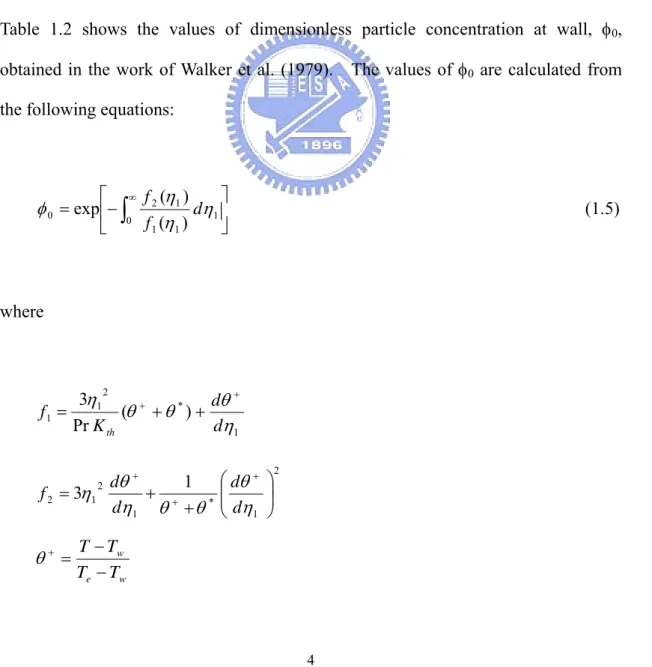
Table 1.2 shows the values of dimensionless particle concentration at wall, φ0,

obtained in the work of Walker et al. (1979). The values of φ0 are calculated from

the following equations:

⎥ ⎦ ⎤ ⎢ ⎣ ⎡ − =

_∫

∞ 0 1 1 1 1 2 0 ) ( ) ( exp η η η φ d f f (1.5) where 1 * 2 1 1 ( ) Pr 3 η θ θ θ η d d K f th + + _{+ +} = 2 1 * 1 2 1 2 1 3 _⎟⎟ ⎠ ⎞ ⎜⎜ ⎝ ⎛ + + = + ₊ + η θ θ θ η θ η d d d d f w e w T T T T − − = + θ

3 / 1 3 / 1 1 9 2 ) 1 ( ⎟ ⎠ ⎞ ⎜ ⎝ ⎛ − = z r Pe_g η

Note that Eq. (1.4) is only applicable before gas temperature is in equilibrium with the wall. In the case of a long tube, they solved the particle transport equation by the particle trajectory method and obtain the exact solution for the thermophoretic deposition efficiency, as shown in Table 1.3. An approximate expression, as can be seen in Table 1.1, was also developed by fitting the exact solutions as a function of PrKth and θ*. The difference between the exact solution and the approximate

solution increases with decreasing PrKth or θ* value, and is less than 18 %.

Batchelor and Shen (1985) also found that the deposition efficiency for the long tube is a function of PrKth and θ*. Their thermophoretic deposition efficiency agrees

well with Walker et al.’s exact solution (1979) only when PrKth = 1. However, when

PrKth and Te/Tw are small, the predicted thermophoretic deposition efficiency does not

agree well with that predicted by Walker at al. (1979).

Stratmann et al. (1994) utilized the SIMPLER algorithm developed by Patankar (1980) to calculate the thermophoretic deposition efficiency and developed an empirical expression for predicting the thermophoretic particle deposition efficiency as shown in Table 1.1.

From the above review, the theory of the thermophoretic deposition efficiency is obviously established for fully developed flow, the entrance flow effect on particle

Table 1.1 Theoretical expressions of thermophoretic deposition efficiency for a long tube where the temperature of hot gas has approached that of the wall.

Walker et al. (1979) Pr ( e w) w th T T T K − = η (approximate solution)

Batchelor and Shen (1985) _⎟⎟

⎠ ⎞ ⎜ ⎜ ⎝ ⎛ ⎟⎟ ⎠ ⎞ ⎜⎜ ⎝ ⎛ − − + ⎟⎟ ⎠ ⎞ ⎜⎜ ⎝ ⎛ − = e w e th e w e th T T T K T T T K 1 (1 Pr ) Pr η Stratmann et al. (1994) _⎟⎟ ⎠ ⎞ ⎜ ⎜ ⎝ ⎛ ⎟⎟ ⎠ ⎞ ⎜⎜ ⎝ ⎛ + − + − − = 932 . 0 28 . 0 ) /( 025 . 0 Pr 845 . 0 exp 1 w e w th T T T K η

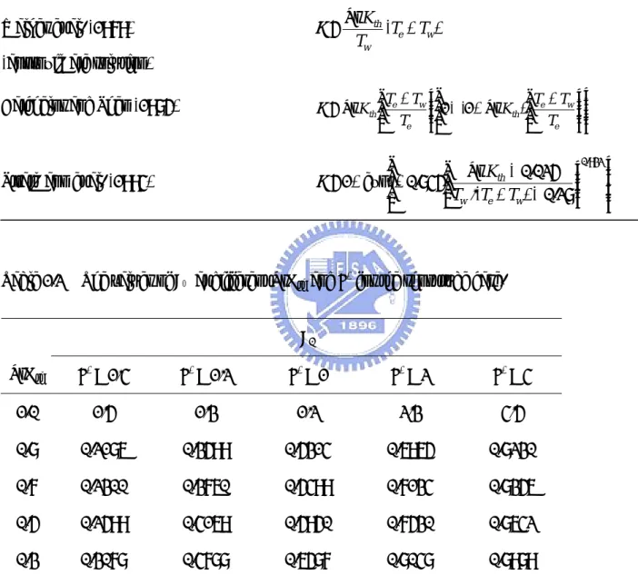
Table 1.2 The values of φ0 at different PrKth and θ* for the short tube case.

φ0 PrKth θ* = 1/4 θ* = 1/2 θ* = 1 θ* = 2 θ* = 4 1.0 1/5 1/3 1/2 2/3 4/5 0.8 0.2186 0.3599 0.5314 0.6965 0.8230 0.7 0.2300 0.3760 0.5499 0.7134 0.8356 0.5 0.2599 0.4169 0.5950 0.7530 0.8642 0.3 0.3078 0.4788 0.6587 0.8048 0.8989

Table 1.3 The exact solution of Walker et al. (1979) for thermophoretic deposition efficiency in the long tube case.

thermophoretic deposition efficiency, %

PrKth θ* = 1/4 θ* = 1/2 θ* = 1 θ* = 2 θ* = 4 1.0 80.0 66.7 50.0 33.3 20.0 0.8 73.0 59.0 42.0 27.0 16.0 0.7 68.0 54.0 39.0 24.0 14.0 0.5 58.0 44.0 30.0 18.0 10.0 0.3 42.0 31.0 20.0 12.0 6.0 θ* _{is dimensionless temperature, T} w/(Te-Tw).

deposition efficiency in tube flow has rarely been investigated. Recently, Fan et al. (1996) found that the gas collection efficiency of an annular diffusion denuder is higher for developing flow than fully developed flow. Since the highest temperature gradient and uniform velocity near the wall occur at the entrance of a tube where both flow and temperature are developing, thermophoretic deposition in the entrance region may be enhanced. Therefore, the first part of this study is to investigate the effect of developing flow in entrance region on the thermophoretic deposition efficiency under laminar flow condition.

1.3 Thermophoretic deposition efficiency in turbulent tube flow

Nishio et al. (1974) and Romay et al. (1998) derived their own expressions for the thermophoretic particle deposition efficiency in turbulent tube flow. They used the one-dimensional control volume approach for the conservation of mass shown in Fig. 1.1 and obtained the following equation:

dz V Q D N dN th t π − = (1.6)

To obtain the thermophoretic velocity, the temperature gradient at the wall was calculated from the following equation:

) ( 0 m w r r g h T T dr dT k = − = (1.7)

Eq. (1.6) was then integrated along the length of the tube. Table 1.4 displays the theoretical expressions of Nishio et al. (1974) and Romay et al. (1998) are shown.

Table 1.4 Theoretical expressions of the thermophoretic deposition efficiency in turbulent tube flow. Romay et al. (1998) th K in p t w e w L T QC hL D T T T ( )exp( / ) Pr 1 _⎥ ⎦ ⎤ ⎢ ⎣ ⎡ + − − − = π ρ η Nishio et al. (1974) _⎟⎟ ⎠ ⎞ ⎜ ⎜ ⎝ ⎛ ⎟ ⎟ ⎠ ⎞ ⎜ ⎜ ⎝ ⎛ ⎟ ⎟ ⎠ ⎞ ⎜ ⎜ ⎝ ⎛ − − − − − = t p m g w e th P L D C u hL T k T T K C ρ ν ρ η 1 exp ( ) 1 exp 4

Figure 1.1 Fluid element.

N N+dN

dz Vth

Both expressions will be used later to predict the thermophoretic deposition efficiency in turbulent tube flow.

Most of the previous researches focused on the thermophoretic deposition in laminar flow regime seem to agree well with the experimental data, however, the study in turbulent tube flow by Romay et al. (1998) found that differences between their theoretical predictions and experimental data existed and increased with the flow Reynolds number. When the flow Reynolds number equaled 5517, the deviationwas about 3 %, and it increases to about 10 % when the Reynolds number was increased to 9656. Similar discrepancy was found when the theoretical predictions of Romay et al. (1998) were compared with the experimental data of Nishio et al. (1974). This indicates that there must be some other mechanisms affecting the deposition especially in the turbulent flow. Romay et al. (1998) argued that the discrepancy may be due to inertially enhanced thermophoresis for laminar flow over curved surfaces (Konstandopoulos and Rosner, 1995) and enhanced thermophoresis caused by non-uniform concentration gradients and reverse thermophoresis in the preparation of heated aerosol source (Weinberg, 1982). Therefore it is worthwhile for this study to obtain more accurate particle deposition efficiency data to validate the theoretical equations of thermophoretic deposition efficiency in turbulent flow regime.

1.4 Isothermal particle deposition mechanisms in tube flow

Besides thermophoresis, there are many other particle deposition mechanisms in tube flow, such as laminar diffusion, particle electrostatic deposition, gravitational settling and turbulent diffusional and inertial deposition. The particle diffusional penetration in laminar tube flow is (Hinds, 1999):

' 77 . 3 ' 50 . 5 1 2/3 ,A = − µ + µ d P , for µ’ < 0.007 (1.8) ) ' 1 . 70 exp( 0975 . 0 ) ' 5 . 11 exp( 819 . 0 ,A = − µ + − µ d P , for µ’ ≥ 0.007 (1.9) where Q DL = '

µ and D=KTB . The particle penetration decreases with an

increasing µ’. When µ’<0.001, the penetration is close to 1.0. When µ’>0.3, the penetration is close to zero and almost all particles deposit on the tube wall.

For submicron particles used in this study, gravitational settling is usually not important while laminar diffusion and electrostatic deposition can be important. Cohen et al. (1995) passed monodisperse singly charged particles through a conducting copper tube (ID= 1.9 cm) and found that particle deposition efficiencies varied from 1 to 4% for particle diameter ranged from 0.015 - 0.095 µm at a mean flow rate of 4.6 l min-1 under laminar flow condition. However the corresponding theoretical efficiencies by Pich (1978) were only from 0.04 to 0.11%. The electrostatic particle deposition efficiency is calculated as (Pich, 1978):

3 / 1 ) 6 ( _e e τ η = (1.10) where 3 0 0 2 4 Fr tC q e πε τ = (1.11) p d F =3πµ' (1.12)

critical particle radial position, rc, to obtain the electrostatic particle deposition efficiency as : 3 3 0 2 0 0 0 3 1 3 1 ln 2 t p E p c c c c D et n K Z r r r r r r r r = − ⎟⎟ ⎠ ⎞ ⎜⎜ ⎝ ⎛ + ⎟⎟ ⎠ ⎞ ⎜⎜ ⎝ ⎛ − + (1.13)

The critical particle radial position is defined such that all particles starting at the tube entrance with r>rc will deposit on the tube wall. After obtaining rc, the particle

deposition efficiency can be calculated as:

2 2 0 1 _⎟⎟ ⎠ ⎞ ⎜ ⎜ ⎝ ⎛ ⎟⎟ ⎠ ⎞ ⎜⎜ ⎝ ⎛ − = r r_c e η (1.14)

Eqs. (1.10) and (1.14) are the expressions for predicting the deposition efficiency of charged particles due to image force. The deposition efficiency due to space charge is derived by Kasper (1981) as:

Et N_e e + − = ′ 1 1 1 η (1.15) where E=4πBq2_.

Ye et al. (1991b) studied the electrostatic deposition efficiency of an annular denuder and found singly charged particles and particles in Boltzmann charge equilibrium had higher deposition efficiency than neutral particles. For example, for a 0.03 µm particle the deposition efficiencies for Boltzmann charge equilibrium

condition and neutral condition are 12.6 % and 2.4 %, respectively, and for a 0.75 µm particle the deposition efficiencies are 4.0 % and 1.5 %, respectively. Some previous investigators who used particles in Boltzmann charge equilibrium as test particles could obtain inaccurate deposition efficiency data for thermophoretic deposition efficiency. That is, even for conductor tubing and for particles that are in Boltzmann charge equilibrium, the deposition efficiency due to electrostatic is still important and must be measured carefully. Therefore, in this study, particles in both Boltzmann charge equilibrium and charge neutral conditions were used and experimental data were compared to see possible influences.

When flow is turbulent, aerosol particles transport toward the inner wall of a tube is substantially enhanced because of eddy diffusion. Friedlander (2000) gave the particle deposition velocity towards the tube wall due to eddy diffusion

) / ( Re 0118 . 0 7/8 1/3 t d Sc D D V = (1.16)

The particle penetration efficiency can be calculated as

) / exp( DV L Q

P_d = −π _{t d} (1.17)

Eq. (1.16) indicates that small particles tend to have higher Vd hence higher

deposition efficiency. This is because small particles (less than 0.1 µm) follow eddy motion easily resulting an increase in wall deposition rate. While large particles greater than 1.0 µm are unable to follow eddy motion smoothly and can be projected to the wall due to inertial force through the relatively quiescent fluid near the tube

surface. This causes deposition rate of large particles to be increased. Such mechanism is called turbulent deposition. Lee and Gieseke (1994) investigated deposition rate of aerosol particles on tube wall under turbulent flow condition. Experimental results of Lee and Gieseke (1994) show that among the existing theories, the theory proposed by Friedlander and Johnstone (1957) is found to be agreed well with their experimental data or the experimental results of Liu and Agarwal (1974) in the regimes of inertial impaction deposition mechanisms. The dimensionless particle deposition velocity of turbulent deposition, developed by Friedlander and Johnstone (1957) is 2 / / 1 6 . 50 ) /( 1883 1 / * ₂ f u V V_{d d} + − = = ₊ + τ , for 0.9 ≤5 + τ 2 / / 1 73 . 13 96 . 0 5 / 9 . 0 04 . 5 ln 5 1 f + − − = + τ , for 5<0.9_τ+ ≤30 2 / f = ，for 50.9_τ+ < _(1.18)

The penetration efficiency is computed using Eq. (1.17).

After reviewing the previous studies, it was found that there still exist some unclear points on the thermophoretic particle deposition efficiency in tube flow. As a result, thermophoretic particle deposition on tube wall under laminar and turbulent flow conditions will be investigated experimentally in this study. The particular geometry of interest was flow through a cylindrical tube where the aerosol was heated to a specified temperature and then cooled by abruptly decreasing the wall temperature to a constant value, and thus a thermophoretic force on the particles was induced causing them to drift toward and deposit onto tube wall. In the experiment,

isothermal deposition mechanisms were also measured first by setting the wall temperature the same as gas flow. In the actual thermophoretic deposition experiment, deposition efficiencies due to isothermal deposition mechanisms can then be assessed and the deposition efficiency due to thermophoresis alone can be obtained accurately.

1.5 Application of thermophoretic force to suppress particle deposition

There are studies on preventing particle deposition on wafer surface. In contrast there is no literature concerning the suppression of particle deposition in a tube flow. In practical application, such as in the semiconductor industry, a common practice is to heat up the tube wall to prevent particle deposition. However, the required wall temperature to effectively suppress particle deposition in the tube is unknown. The last part of this study further conducts numerical analysis to quantify particle deposition efficiency using different tube wall temperatures that are higher than the inlet gas flow under laminar tube flow condition. The numerical results will then be verified with the experimental data. The numerical results will also be used to develop an empirical expression for predicting the minimum wall temperature needed to effectively suppress diffusional particle deposition by thermophoretic force.

To reduce particle deposition on wafer surface, thermophoretic force is usually used, e.g., by Stratmann et al. (1988), Ye et al. (1991a) and Bae et al. (1995). Stratmann et al. (1988) derived an expression for the thickness of the dust-free layer for flow over a free-standing wafer. As the temperature gradient at the wall and the velocity component normal to the wall were known, the particle equation of motion obtained from the equilibrium of inertial force, drag force and thermophoretic force

on the particle was solved to find the thickness of the dust-free layer near the forward stagnation point of the wafer surface. According to Stratmann et al. (1988), the analytical expression of the dust free layer thickness is,

189 . 0 2 / 1 2 / 1 2 / 1 Pr 961 . 0 _⎥ ⎦ ⎤ ⎢ ⎣ ⎡ − ⎟ ⎠ ⎞ ⎜ ⎝ ⎛ = ∞ w w th df T T T K a v δ (1.19)

The above equation states that the dust-free layer thickness depends on the temperature difference between the gas flow and wafer surface. However, there is no analytical solution available yet for thermophoretic particle deposition velocity at an arbitrary temperature difference. Based on Eq. (1.19), δdf for aluminum and

copper particles (0.5< dp < 2µm) for a temperature differences as small as 10 °C was

found to range from 100 to 200 µm, which was thick enough to prevent particle deposition.

Ye et al. (1991a) used the SIMPER algorithm to solve the coupled Navier-Stokes, energy and convection-diffusion equations to obtain the velocity, temperature and concentration fields. The convection-diffusion equation took into account the external forces of sedimentation and thermophoresis. The measured particle deposition velocity on the wafer surface was found to decrease with an increasing temperature of the surface, and agree with the numerical results. It was shown that by heating the wafer surface to a temperature 10 °C higher than the air flow, a clean zone between 0.03 to 1.0 µm particles was created. The experimental study of Bae et al. (1995) also showed that by raising the wafer surface temperature by 5 °C higher than the surrounding air, the average deposition particle velocity in the range from 0.1 to 1 µm in diameter was reduced to less than 10-4 _cm/s.

1.6 Objectives of this study

The objectives of this study are summarized as:

1. To investigate the effect of developing flow at entrance region on thermophoretic particle deposition efficiency numerically.

2. To investigate the effect of particle electrostatic charge on thermophoreic particle deposition efficiency in tube flow under laminar and turbulent flow conditions experimentally.

3. To conduct numerical analysis and experiments to study thermophoretic effect on particle deposition efficiency in laminar tube flow.

CHAPTER 2

NUMERICAL METHODS

In section 2.1, the temperature fields obtained either from the analytical solution or numerical simulation are discussed. Then the critical trajectory method for calculating the thermophoretic particle deposition efficiency is presented. In the last section of this chapter, the method used to solve convection-diffusion equation to obtain particle deposition efficiency when the temperature of tube wall is higher than gas flow is described.

2.1 Temperature field

In laminar flow, the entry length for the velocity profile to become fully developed given by Incropera and De Witt (1996) is

Re 05 . 0 ≅ ⎟⎟ ⎠ ⎞ ⎜⎜ ⎝ ⎛ dep t D z (2.1)

and the entry length for the temperature profile to become fully developed is (Kays and Crawford, 1980) g dep t Pe D z 05 . 0 Pr Re 05 . 0 = ≅ ⎟⎟ ⎠ ⎞ ⎜⎜ ⎝ ⎛ (2.2)

That is, temperature is fully developed earlier than velocity when Pr < 1. In case that thermal entrance length is much shorter than the total tube length, one can

assume that temperature is fully developed.

Fully developed flow and temperature fields

The case of the fully developed flow and temperature fields is discussed first. When temperature is fully developed, the dimensionless temperature profile (Tw-T)/(Tw-Tm) is invariant in the axial direction, and is a function of radial

coordinate only. When the dimensionless distance Z is greater than the dimensionless thermal entry length, the invariant temperature profile can be expressed as (Skelland, 1974).

(

+

)

= ∞ = = + ∞ = = + + − ⎟⎟ ⎠ ⎞ ⎜⎜ ⎝ ⎛ − − = − − +

∑

∑

z dr d B z r B T T T T j r j j j j j j j j j j m w w 2 1 1 2 1 2 exp 4 ) exp( ) ( β φ β β φ (2.3) where 0 r r r₊ =

,

Pr Re /r0 z z₊ =

∑

=∞ = + + = i i i ji j r r 0 ) (

α

φ

,

α

ji

=

0

for i <0 1 = ji α for i = 0, 2 4 2 2 / ) ( _{i i} i j ji =−β α− −α − α 3 8 ) 1 ( 4 − + = j j β ；j=1,2,3,… 3 2 1 _2.84606 ) 1 (₋ − _× − = j _j j B β

3 1 1 01276 . 1 2 − = + = ⎟⎟ ⎠ ⎞ ⎜⎜ ⎝ ⎛ − + j r j j dr d B β φ

The polynomial function obtained from curve fitting the calculated temperature profile from Eq. (2.3) is

805 . 1 041 . 0 487 . 3 734 . 1 2 3 + ⎟⎟ ⎠ ⎞ ⎜⎜ ⎝ ⎛ − ⎟⎟ ⎠ ⎞ ⎜⎜ ⎝ ⎛ − ⎟⎟ ⎠ ⎞ ⎜⎜ ⎝ ⎛ = − − o o o m w w r r r r r r T T T T (2.4)

Eq. (2.4) is then used to obtain the temperature gradient, and the corresponding thermophoretic velocity for this case.

Fully developed flow and developing temperature

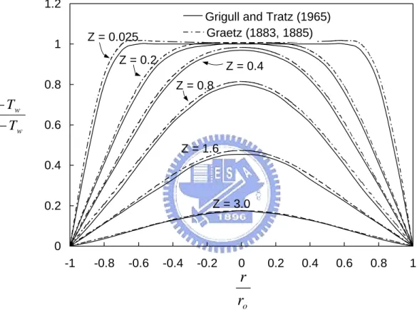
For the developing temperature profile, the analytical solution of Graetz’s problem is (Skelland, 1974)

∑

=∞ = + + − = − − j j j j j e w w z r B T T T T 1 2 ) exp( ) ( β φ (2.5)

The dimensionless developing temperature profiles of Eq. (2.5) are compared with that described in Grigull and Traz (1965) and found both profiles agree very well, as indicated in Fig. 2.1.

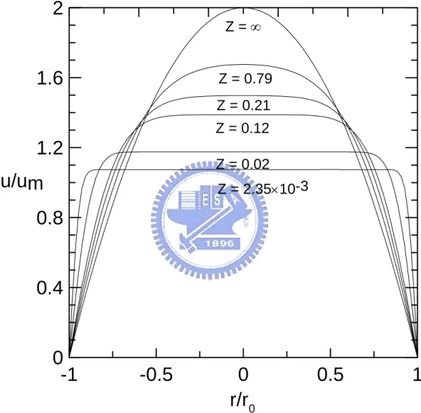
Developing flow and temperature

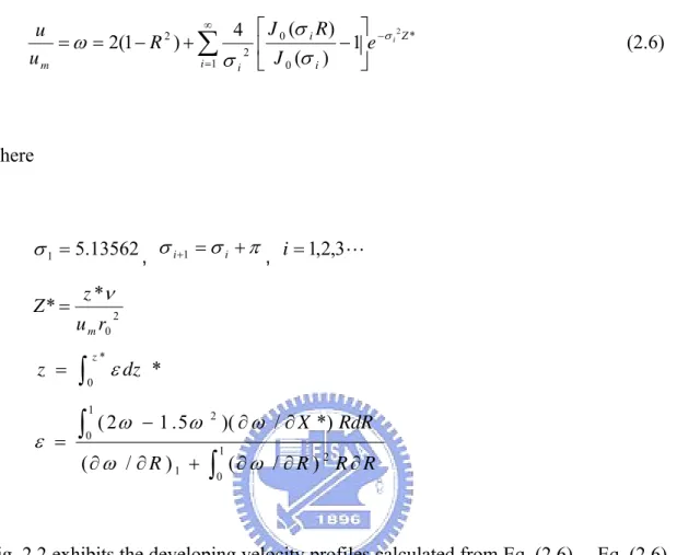
two-dimensional developing velocity field derived by Sparrow et al. (1964) was used: * 1 0 0 2 2 ₁ 2 ) ( ) ( 4 ) 1 ( 2 Z i i i i m i e J R J R u u _σ σ σ σ ω ∞ − =

∑

⎥ ⎦ ⎤ ⎢ ⎣ ⎡ − + − = = (2.6) where 13562 . 5 1 = σ _, σi 1₊ =σi +π_, i=1,2,3" 2 0 * * r u z Z m ν =

∫

= * 0 * z dz z ε

∫

∫

∂ ∂ ∂ + ∂ ∂ ∂ ∂ − = ₁ 0 2 1 1 0 2 ) / ( ) / ( *) / )( 5 . 1 2 ( R R R R RdR X ω ω ω ω ω ε

Fig. 2.2 exhibits the developing velocity profiles calculated from Eq. (2.6). Eq. (2.6) was then used to calculate the developing temperature field for developing flow numerically by solving the following 2-D cylindrical energy equation:

⎟⎟ ⎠ ⎞ ⎜⎜ ⎝ ⎛ ∂ ∂ + ∂ ∂ = ∂ ∂ + ∂ ∂ 2 2 1 r T r T r r T v z T u α (2.7)

where the boundary conditions are

e T r T( ,0)= ; T(r0,z)=Tw; _∂ (0, )=0 ∂ z r T

In the numerical simulation for developing temperature field, the finite volume method and SIMPLE algorithm (Patankar, 1980) were used. In the test run, the number of grid in the computational domain was either 4,000 (100 in the axial direction × 40 in radial direction), 12,000 (200 in the axial direction × 60 in radial direction) or 24,000 (300 in the axial direction × 80 in radial direction). The numerical results indicate that the number of grid of 12,000 is accurate enough and was adopted in the further study. The cell spacing is finer near the wall and inlet where temperature gradients in radial direction are expected to be larger. In the simulation, the influence of radial fluid velocity and temperature-dependent fluid properties on thermophoretic deposition efficiency was accounted for.

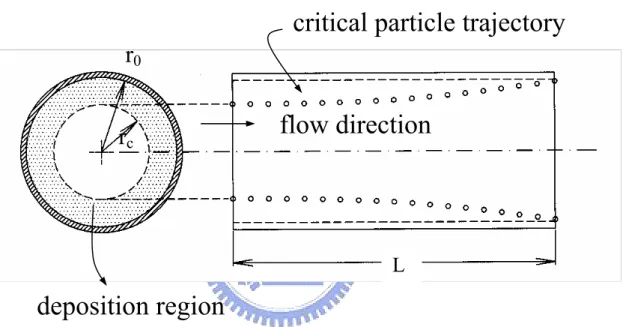
2.2 Critical particle trajectory method to calculate thermophoretic particle deposition efficiency

The critical particle trajectory method is used to obtain the thermophoretic particle deposition efficiency when neglecting particle diffusion. The critical particle trajectory is shown in Fig. 2.3. A particle starts at the critical radial position, rc, at the entrance will deposit just at the end of the tube of length L. The

annular-hatched region from rc to r0 is the particle deposition region where a particle

starts will deposit somewhere on the wall of the tube. When flow is fully developed, analytical temperature field is available and the particle equations of motion can be solved to obtain the critical radial position and the thermophoretic deposition efficiency. However, when both flow and temperature are developing (or combined developing case), there is no analytical equation for temperature field. In this study, it is found that developing velocity field simulated numerically by finite difference

0 0.2 0.4 0.6 0.8 1 1.2 -1 -0.8 -0.6 -0.4 -0.2 0 0.2 0.4 0.6 0.8 1 數列1 數列2 o

r

r

Z = 0.025 Z = 0.2 _{Z = 0.4} Z = 0.8 Z = 1.6 Z = 3.0 Graetz (1883, 1885) Grigull and Tratz (1965)

w e w T T T T − −

Figure 2.1 Comparison between Graetz’s solution and temperature profile in the thermal entry region with that of Grigull and Tratz (1965).

-1

-0.5

0

0.5

1

r/r

₀

0

0.4

0.8

1.2

1.6

2

u/um

_{Z = 2.35×10-3}

Z = 0.02

Z = 0.12

Z = 0.21

Z = 0.79

Z = ∞

Figure 2.3 Critical particle trajectory.

r

c

r

0

critical particle trajectory

flow direction

L

method is not accurate. Therefore, the analytical velocity distribution developed by Sparrow et al. (1964) was used to calculate the developing temperature profile numerically, and then the critical particle trajectory and deposition efficiency was obtained by solving the particle equations of motion.

In the cylindrical coordinate, the particle equations of motion in the z (radial) and r (axial) directions are respectively

(

)

τ dt dz u C dt z d p d / 24 Re 2 2 ₋ = (2.8) and

(

)

p th p d Bm V dt dr v C dt r d + − = τ / 24 Re 2 2 (2.9)

where Cd is the drag coefficient proposed by Rader and Marple (1985),

) Re 0916 . 0 1 ( Re 24 p p d C = + , Rep < 5 (2.10) and ) Re 158 . 0 1 ( Re 24 2/3 p p d C = + , 5 < Rep < 1000 (2.11)

To calculate the values of B and τ in Eq. (2.9), the C value, slip correction factor, should be calculated first. A fitted expression of C values to air data for particles is given by Allen and Rabbe (1985) as

)] / exp( [ 1 Kn a b c Kn C= + + − (2.12)

For solid particles, a=1.142, b=0.558 and c=0.999 (Allen and Rabbe, 1985) while for oil droplets, a=1.207, b=0.440 and c=0.596 (Rader, 1990). It is noted that the deviation of C values between these two materials is very small, which is less than 4.1 % for particle sizes in the range of 0.001 to 1 µm at temperature of 293 K and pressure of 1 atm. Therefore, we decide to use the equation provided by Allen and Rabbe (1985) to calculate the C value.

In order to calculate thermophoretic deposition efficiency, the critical radial position of particle trajectory, rc, should be known. For the combined fully

developed case, the analytical equation listed in the appendix A, Eq. (A.6), is solved to obtain rc and the corresponding efficiency. For fully developed flow and

developing temperature case, the particle equations of motion have to be solved numerically by the fourth order Runge-Kutta method. For the combined developing case, the particle equations of motion of Eqs. (2.8) and (2.9) were integrated numerically by means of the fourth order Runge-Kutta method. As the particle equations of motion are integrated through the domain of interest, initial velocity is given equal to the average gas flow velocity, and the initial position is set at the entrance of the tube. The new particle position and velocity after a small increment of time is calculated by numerical integration. The procedure is repeated until the particle hits the tube wall or leaves the calculation domain.

After obtaining the critical radial position, rc, the efficiency of thermophoretic

deposition for fully developed flow is calculated in the following equation assuming the particle concentration is uniform at the inlet,

4 0 2 0 2 0 2 0 2 2 1 2 1 2 0 ⎟⎟ ⎠ ⎞ ⎜⎜ ⎝ ⎛ + ⎟⎟ ⎠ ⎞ ⎜⎜ ⎝ ⎛ − = ⎟⎟ ⎠ ⎞ ⎜⎜ ⎝ ⎛ − =

∫

r r r r r u rdr r r u c c m r r m f c π π η (2.13)

For the combined developing case, besides assuming uniform particle concentration, the velocity profile is known to be uniform at the entrance of the tube, and the deposition efficiency can be calculated as

2 0 1 _⎟⎟ ⎠ ⎞ ⎜⎜ ⎝ ⎛ − = r rc d η (2.14)

2.3 Solutions of convection-diffusion equation to obtain thermophoretic particle

deposition efficiency

For predicting particle deposition efficiency in a circular tube, the fully developed flow field was used. The temperature field was obtained numerically from energy equation, Eq. (2.7), by controlling the temperature of tube wall either higher or lower than gas flow.

Particle concentration field was obtained numerically by solving the following particle convection-diffusion equation:

) ( ) ( ) (uKN =∇⋅ D∇N −∇⋅ VK_thN ⋅ ∇ (2.15)

e N r N( ,0)= ; N(r₀,z)=0; (0, )=0 ∂ ∂ z r N (2.16)

In Eq. (2.15) the thermophoretic coefficient Kth, Eq. (1.3), proposed by Talbot et al.

(1980) was used to calculate thermophoretic velocity, VK_th.

The particle convection-diffusion equation was also solved by the finite volume method using SIMPLE algorithm (Patankar, 1980). In the test run, three different numbers of grids in the computational domain: 4,000 (100 in the axial direction × 40 in radial direction), 12,000 (200 in the axial direction × 60 in radial direction) or 25,200 (280 in the axial direction × 90 in radial direction) were used. The numerical results showed that the number of grid of 12,000 was accurate enough and was adopted in the further study.

CHAPTER 3

EXPERIMENTAL METHODS

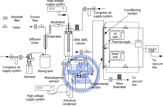
The experimental setup for particle deposition experiment is shown in Fig. 3.1 while that for suppression experiment is illustrated in Fig. 3.2. The experimental system consists of three parts: (1) the aerosol generation and conditioning section, which produces monodisperse aerosol with known diameter with a predetermined temperature; (2) the experimental section, which establishes a temperature gradient between the tube wall and gas to induce or suppress particle deposition on tube wall by thermophoresis; and (3) temperature, flow and particle measurement systems, which measure the particle deposition efficiency at a certain flow rate and temperature gradient.

3.1 Aerosol generation and conditioning

The aerosol was generated by a Collison atomizer and mixed with clean dry air in a mixing tank, and then passed through a silica gel diffusion dryer. After drying, the aerosol was neutralized by a TSI 3077 electrostatic charge neutralizer. After neutralization, the aerosol was passed through a differential mobility analyzer (DMA; TSI 3081 Long DMA column) where a high-voltage was applied to select particles of a known electrical mobility. The monodisperse aerosol from the DMA was neutralized again and mixed with clean dilution air in another mixing tank to conduct experiment for particles in Boltzmann charge equilibrium. For the experiment involving only completely charge neutral (or zero charge) particles, an electrical condenser was used between the neutralizer and mixing tank to remove all charged particles.

Oil bath Water bath Excess flow Atomizer Diffusion Dryer To vaccum line Conditioning Section Experimental section Thermocouple CNC To vaccum line Mass flowmeter Monodisperse aerosol Compress air supply system Neutralizer High-voltage supply system Mixing tank DMA 3081 column Rotameter Valve Absolute filter Compress air supply system High-voltage

supply system _Electrical condenser

Oil bath Water bath Excess flow Atomizer Diffusion Dryer To vaccum line Conditioning Section Experimental section Thermocouple CNC To vaccum line Mass flowmeter Monodisperse aerosol Compress air supply system Neutralizer High-voltage supply system Mixing tank DMA 3081 column Rotameter Valve Absolute filter Compress air supply system High-voltage

supply system _Electrical condenser

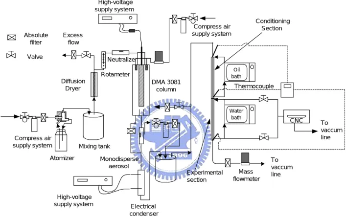
3.2 Experimental system

The experimental system was further divided into two parts: (1) the conditioning section: the monodisperse aerosol stream was passed through the conditioning section, which was heated to a desired temperature by a heat exchanger for deposition experiment (i.e. thermostated silicon-oil bath). However, for suppression experiment, the temperature of conditioning section was kept constant (296 K), (2) the experimental section: for deposition experiment, the tube wall temperature was kept at 296 K by another heat exchanger (thermostated water bath) to establish a temperature gradient between the gas and wall of the tube in order to induce deposition by thermophoresis. For suppression experiment, the tube wall-temperature of this section was heated to a desired temperature to get the zero deposition. The tube lengths of the conditioning and experimental section are 1.56 and 1.18 m, respectively, with an inner tube diameter of 0.0043 m.

Three thermocouples−at the inlet of conditioning section, at the outlet of the experimental section, and at the junction between the conditioning section and experimental section−were installed to monitor the temperature at these points of the aerosol stream. The aerosol coming out from the experimental section was passed through a filter and then mass flow-controlling device (MKS Instruments, Inc.) before it was exhausted into a vacuum line. The aerosol concentrations at the inlet and at the outlet of the experimental section was measured using TSI-3760 cleanroom condensation nucleus counter (CPC), which had a sample flow rate of 1.5 l min-1.

For the deposition experiment, the particle material used was NaCl. Normally 0.5 % w/v aqueous solution of NaCl was usually used. The concentration was

increased to about 1.5 % for the larger particle sizes (dp> 0.35 µm) investigated.

While for the suppression measurement, the particles used were NaCl or oleic acid generating from 1.0 % w/v aqueous NaCl solution or 2 %, v/v oleic acid dissolved in alcohol. Mass flow controller, rotameter and CPC were calibrated prior to experimental studies. Particle size distributions for the material used, were carried out to check the DMA performance. Leak test was performed some time in between the experiments to prevent the particle loss by leaking and the particle contamination from ambient air (however the experiment was carried out at ambient pressure). The flow rate of sheath air and polydisperse aerosol stream to DMA was kept constant, i.e. 5 and 0.5 l min-1, respectively, through out the study.

3.3 Experimental procedure

Aerosol material solution was taken in atomizer and then turned on the atomizer. The applied voltage in voltage-supplier was adjusted to get the particle of desired size from DMA. The experimental section flow rate was then set using the downstream mass flow controller and the dilution air flow valve. For the deposition studies, the gas temperature at the conditioning section was heated to a desired value using the heat exchanger, while the temperature of the experimental section was kept constant (296 K) throughout this study. After stabilizing the conditions of the system, the particle concentrations at the inlet of the conditioning section and the outlet of experimental section were measured to determine the total deposition efficiency by CPC using operating the inlet and outlet valve. After deducting deposition efficiencies due to other particle deposition mechanisms from the total deposition efficiencies, the experimental thermophoretic deposition efficiency can be obtained. During the measurement process, it was found that the isothermal deposition in the

conditioning section could be suppressed completely when the tube wall temperature was heated higher than 343 K, which was the minimum temperature in the conditioning section. Therefore, it is not necessary to consider particle deposition losses in this section.

Whereas, for suppression studies, the temperature of conditioning section was kept constant (296 K), and the temperature of experimental section was heated to the desired temperature from 296 to 315 K by heat exchanger with a thermostated water bath to establish a temperature difference between the gas and the tube wall for the particle deposition suppression experiment. The particle deposition efficiency at a certain flow rate and particle diameter was determined from the particle number concentration data at the inlet and outlet of the experimental section. The deposition efficiency due to pure laminar flow convection diffusion was first obtained when the tube wall and aerosol stream were both kept at the temperature of 296 K. Then the tube wall temperature was raised to a desired temperature for determining the reduced deposition efficiency due to thermophoresis. The test was repeated for different flow rates and particle sizes.

The above procedure was repeated for different flow rates and particle sizes. For one data at particular test condition, average deposition from 6-8 data sets was taken, where each set contained 10 readings of the inlet, and of the outlet. The measurement time was 1-2 min/10 readings excluding system stabilization time, which was varied anywhere from 20-100 sec/reading. After completion of one data set reading, the experimental section was cleaned by passing clean air through it. The experimental conditions tested are given in Table 3.1 for deposition experiment and Table 3.2 for suppression experiment.

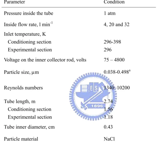
Table 3.1 Experimental conditions of deposition measurement.

Parameter Condition Pressure inside the tube 1 atm

Inside flow rate, l min-1 4, 20 and 32 Inlet temperature, K

Conditioning section Experimental section

296-398 296 Voltage on the inner collector rod, volts 75 – 4800

Particle size, µm 0.038-0.498a Reynolds numbers 1340–10200 Tube length, m Conditioning section Experimental section 2.74 1.56 1.18

Tube inner diameter, cm 0.43

Particle material NaCl

a _{There are 18 particle sizes in the deposition experiment. They are 0.038, 0.054,}

0.08, 0.1, 0.118, 0.136, 0.152, 0.17, 0.19, 0.214, 0.26, 0.294, 0.33, 0.364, 0.397, 0.431, 0.464 and 0.498 µm in diameter.

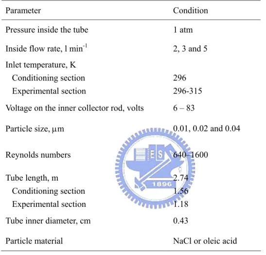
Table 3.2 Experimental conditions of suppression measurement.

Parameter Condition Pressure inside the tube 1 atm

Inside flow rate, l min-1 2, 3 and 5 Inlet temperature, K

Conditioning section Experimental section

296 296-315 Voltage on the inner collector rod, volts 6 – 83

Particle size, µm 0.01, 0.02 and 0.04

Reynolds numbers 640–1600 Tube length, m Conditioning section Experimental section 2.74 1.56 1.18

Tube inner diameter, cm 0.43

CHAPTER 4

ENTRANCE EFFECT ON THE THERMOPHORETIC DEPOSITION EFFICIENCY

4.1 Thermophoretic deposition efficiency for fully developed temperature and velocity fields

Fig. 4.1 compares the thermophoretic deposition efficiency of the present study and previous theories at a flow rate of 5 l min-1 for the pipe geometry described in the experiment of Romay et al. (1998). The fluid and particle properties used in the calculation were estimated at the averaged temperature of inlet gas and tube wall. The tube length is 0.905 m, tube diameter is 0.0049 m and the Reynolds number of the gas flow equals 1423 which is in the laminar flow region. The thermal conductivity is 6.0 W/(mK) for NaCl particle (Romay et al., 1998). Fig. 4.1 shows that the deposition efficiency of submicron particle agrees well with the prediction of Stratmann et al. (1994) and Batchelor and Shen (1985) for the long tube, the deviation is smaller than 2 %. It can be seen that the thermophoretic deposition efficiency increases at first with an increasing inlet gas temperature and decreasing particle size, but when particle size is further decreased to 0.05µm and 0.03µm, the thermophoretic deposition efficiency remains almost the same (Fig. 4.1). In Fig. 4.2, the deposition efficiency calculated by the expression of Stratmann et al. (1994) (see Table 1.1) is compared with the present study. It shows the present theory is in very good agreement with the expression of Stratmann et al. (1994).

250

300

350

400

450

500

0

5

10

15

20

25

Stratmann et al., (1994)

This study

Batchelor and Shen (1985)

Gas temperature at tube entrance (K)

The

rmopho

re

tic

depo

s

itio

n

efficien

cy, %

Particle material : NaCl

Pipe diameter : 0.49 cm

Pipe length : 0.905 m

Wall temperature = 293 K

Re = 1423

0.1 µm

0.5 µm

Figure 4.1 Comparison of theoretical deposition efficiency with previous theories in laminar tube flow.

0

2

4

6

8

10

12

14

16

18

0.001

0.01

0.1

1

數列1 數列2

Thermophoretic deposition efficiency, %

Stratmann et al., (1994)

This study

1

β

Figure 4.2 Comparison of present theoretical thermophoretic deposition efficiency with numerical prediction of Stratmann et al. (1994) in laminar tube flow.