J
OURNAL
of the
A
SIAN
R
EAL
E
STATE
S
OCIETY
1998 Vol. 1 No 1: pp. 81 - 100
Aggregated Needs and the Location Choice
of Households in Taipei
Chin-Oh Chang
Department of Land Economics, National Chengchi University, Taipei, Taiwan, or [email protected]
Shu-Mei Chen
Department of Land Economics, National Chengchi University, Taipei, Taiwan.
Shiawee X. Yang
College of Business Administration, Northeastern University, Boston, MA USA 02115 or [email protected]
This paper examines the impact of aggregate d needs of household members on the choice of housing location in Taipei, Taiwan, using a sample of 11,191 households and information collected from the 1990 Census of Population and Housing. Our results indicate that the choice of housing location is significantly affected impacted by the age, family origin, past housing location, education and occupation status, and the location of the workplaces of both spouses. We also find that this decision is more significantly influenced by the attributes of the m ale spouse than the female. However, among the households with a female household head, the female spouse characteristics are more likely to be significant. Our results also offer a snapshot of today’s Taiwanese culture and shows that it is dramatically different from the commonly believed male-dominated traditional Chinese culture.
Keywords
1.
Introduction
Most housing choice theories are based on mainstream microeconomic theories. Each household seeks a balance between employment, housing, location, and transportation facilities. According to these demands, households choose the housing location according to their characteristics to maximize utilities and subject to affordability. Furthermore, consumers are expected to make housing decisions after obtaining sufficient market information (Tu and Goldfinch, 1996). The household location decision-making process has been studied for many cities and countries in the world. In light of existing theories, this paper attempts to examine the household location decision for the city of Taipei, Taiwan.
There are two main objectives of this paper. Firstly, this paper is to explore the impact of the household characteristics on housing location in the city of Taipei. Families prefer to live in locations with the greatest number of amenities, including accessibility. Since families are unique in age, education, occupation status, etc., their criteria of selecting the housing location may be heavily influenced by these characteristics. This paper improves upon the existing studies (Fu, 1984; Lin, 1990; Liu, 1996, and Chen, 1997) by carefully treating the location variable and related econometric tests.1 Dividing Taipei City into six areas by municipal districts, geographical locations and the rank in average housing prices, we make the location choice variable to have six ordered threshold values. Order response Probit models are employed to test the six alternative locations in a joint fashion.
Secondly, this paper is to examine the gender role in the household location decision. What makes Taipei unique in housing location choice is the strong influence of a traditional Chinese culture. A noticeable characteristic of the Chinese culture is the dominant role of husbands in household decision making. In China, women traditionally have an inferior position to men in a household, unlike contemporary western society (e.g., the US) where households enjoy greater gender equality. A household with gender equality is expected to choose its housing location based on the aggregate demands of each individual member of the household.2 How does a family in today’s Taiwanese society make such a decision? This paper attempts to
1
For example, Liu (1996) simply divides the Taipei City area into three areas, the old city area, the new city area and the newly developed area.
2
In a democratic society, a family is the unit of labor supply and decision making formed from consumer behavior. A household works for survival together, so many of family affairs are jointly decided by each member of the household, no decision is born from the independent uncoordinated decision of a single family member (Chang et al., 1993). In a well-balanced family, husband and wife jointly make most decisions.
answer this question. Specifically, it analyzes the demands of both male and female spouses in a family, and how this affects the choice of housing location.
Existing housing demand and housing choice studies seldom draw attention to the needs of individual household members. Most studies in this area take into account only the characteristics of the household head as the determinant of household locations. Only a few related studies have been concerned about the role of the female spouse in the family decision-making process (Samsinar, 1994, and Williams, 1990). We argue that the housing choice model based on the household head characteristics alone cannot reflect the entire household’s housing needs. In actual housing choice behavior, each household member, and especially the spouse of the household, affects the decision of housing location. Our paper makes a significant contribution by introducing the same set of characteristics for both male and female spouses in a household as explanatory variables in the ordered-response Probit model. Furthermore, we divide the sample into two sub-samples: households with a male household head and households with a female household head. The maximum likelihood models are applied to the entire sample and sub-samples. The decision making power of the male and female spouses can thus be jointly examined.
References concerning women’s housing needs focuses on the role of women in the housing choice decision-making process. In a patriarchal economic system, women face inequality in both salary and job position. They also have limited house-owning opportunities and locations for selection. They cannot obtain satisfaction in mass transportation accessibility and needs for child care services (Cook and Rudd, 1984; Munro and Smith, 1989, and Smith, 1990). Moreover, the desire for women to take the risk of living in unfamiliar environments is not strong, and, as a result, they seldom move away from their environment.
As women increase their financial resources and earning capacity, the existing roles of women in the household decision making process must be reexamined. Since these resources may have become more needed by their families, or to some extent, have become as important as the man’s resources, women are more capable of controlling their own lives and making their own decisions. Therefore, women’s financial resources have become a foundation for decision-making power within the household (Baber and Allen, 1992). Questions arise from this foundation. Lin et al. (1996) find that the “family wage” made it impossible for men and women to have equal income levels in this patriarchal social system.3 Even after
3
Lin et al. (1996) discusses feminist ideology and traditions in Taiwanese society. They examine ways to improve knowledge for females in the society, and discuss how to establish a new culture and new society founded on gender equality. This
women participated in the labor market, the traditional gender division of labor in household chores remains the same. This gender-role ideology has restricted the woman’s financial rights in the family. Particularly, performing unpaid housework deprives the spouse of the right to the control financial resources. In some circumstances, even if women can control financial resources, they still do not give priority to their own needs.4 The husband remains the final decision-maker regarding major decisions.
Through the economic development in the past half of century, the Taiwanese society has changed dramatically. Double-income families are gradually becoming common in the modern-day society. Therefore, should the decision-making process for household location depart from the traditional mode? Also, are younger spouses less likely affected by the traditional gender-role ideology that restricts women? Do these younger female spouses play a more aggressive role in the housing location decision-making process than their older counterparts? Increasingly there are more spouses that have a higher education and occupation status, and higher income levels; they make greater financial contributions to the family. Does this financial contribution serve as a foundation to allow the spouse to have a stronger influence in the household? Do female household heads make different housing location choices than households having male household heads? These are the questions that this paper attempts to answer with empirical evidence.
The paper is laid out as follows. Section II discusses the empirical data, explanatory variables, and estimation models. In Section III, empirical results are presented and analyzed. The last section concludes the study.
2.
Data and Empirical Modeling
We group together some neighboring administrative districts in the city of Taipei to form six districts that are utilized as the alternative location choice variable. These districts are: Central Area One (Hsin-I and Sungshan), Central Area Two (Chungchen, Ta-An and Chungshan), Eastern (Neihu and Nankang), Western (Tatung and Wanhwa), Southern (Wenshan), and Northern (Shihlin and Peitou).
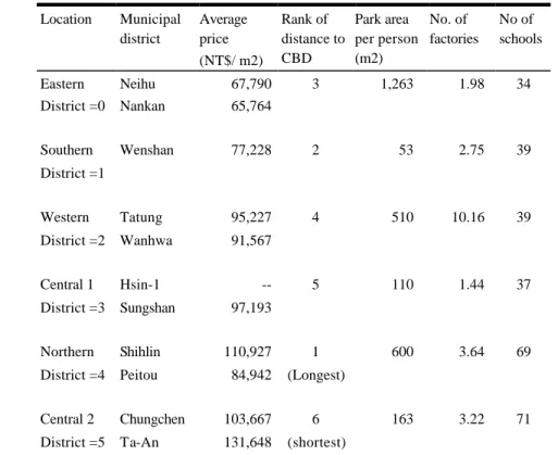
These areas in Taipei City area are distinguished by housing prices, distance to the central business district, and living amenities (Table 1). The characteristics of the six areas are introduced below:
paper, however, focuses only on women’s position in residential location decision-making rights within the households.
4
This is demonstrated by Bielby and Bielby (1992), Camstra (1996) and Yu et al., (1996).
• The Central 2 District is the central business and financial district. It is located near the early-developed center of Taipei City. It has the highest average housing price among all areas.
• The Northern District is a suburban area where many businesses and factories are located. It is famous for its good living environment, with the second highest green/garden areas. The housing price is the second highest.
• The Central 1 District is the new central city area, businesses have gradually shifted here from the Central 2 District. Housing prices are not as high as in the previous two areas.
• The Western District is the earliest developed area of Taipei City. There is a lower concentration of households of Mainland Chinese descendants. The housing prices are in the middle range, similar to the
Central 1 District.
• The Southern District and the Eastern District are the far suburbs of Taipei with considerably longer commuting time and distances than other areas. The housing prices are relatives low.
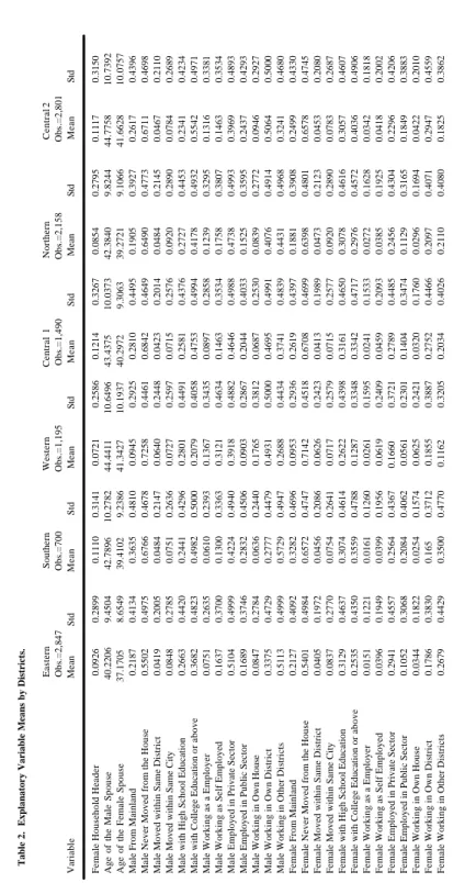
The descriptive statistics of these explanatory variables of each district are shown in Table 2, and the aggregated data for the entire sample can be seen in Table 3. We observe the following preliminary information.
In each district, approximately 90% of the household heads are male. However, in the Southern District and Central Districts 2 and 1 of the central city area, the ratio of female household heads is higher, 11, 11 and 12 percent.
In the recently developed Eastern District, younger households are the largest percentage. The average age of husbands and wives are 40.22 and 37.17, relative to 42.81 and 39.70 for the entire sample. The Western District is the traditional old city area, and has a higher percentage of older households, as has the Central 2 District. The Southern District has the highest percentage of Mainland Chinese descendent households, 36.35 percent for male household heads and 32.82 percent, for female. On the other hand, the older Western District has the most Taiwanese descendent households (9.5 percent mainland descendents).
Table 1. Basic Characteristics of the Variables
Source: 1. The average price of each district comes from the survey data of Ti-Lian Housing Market, No.195, February 1991, Taipei, Taiwan.
2. The others come from the Statistical Abstract of Taipei Municipality, Taipei Municipal Government,1992.
The majority of households have not moved during the past five years. This especially holds true for the households in the Western District (72.58 percent not moved), where the traditional Taiwanese household probably will continue to live in their existing homes. On the contrary, the Eastern District has the highest mobility; only 54 (female) to 55 (male) percent of the residents have lived there for five years or longer. The data revealed that most of the households that moved from other locations within Taipei City moved revealed that most of the households that moved from other locations within Taipei City moved to the newly developed Eastern area. Both spouses in the Western and two Central Districts have a higher rate to be employers than other locations. However, there are more self-employed living in the Western District.
Location Municipal district Average price (NT$/ m2) Rank of distance to CBD Park area per person (m2) No. of factories No of schools Eastern Neihu 67,790 3 1,263 1.98 34 District =0 Nankan 65,764 Southern Wenshan 77,228 2 53 2.75 39 District =1 Western Tatung 95,227 4 510 10.16 39 District =2 Wanhwa 91,567 Central 1 Hsin-1 -- 5 110 1.44 37 District =3 Sungshan 97,193 Northern Shihlin 110,927 1 600 3.64 69
District =4 Peitou 84,942 (Longest)
Central 2 Chungchen 103,667 6 163 3.22 71 District =5 Ta-An 131,648 (shortest)
Table 2. Explanatory Variable Means by Districts.
Eastern Southern Western Central 1 Northern Central 2 Obs.=2,847 Obs.=700 Obs.=1, 195 Obs.=1,490 Obs.=2,158 Obs.=2,801 Variabl e Mean Std Mean Std Mean Std Mean Std Mean S td Mean Std
Female Household Header
0.0926 0.2899 0.1110 0.3141 0.0721 0.2586 0.1214 0.3267 0.0854 0.2795 0.1117 0.3150
Age of the Male Spouse
4 0.2206 9.4504 42.7896 10.2782 44.4411 10.6496 43.4375 10.0373 42. 3840 9.8244 44.7758 10.7392
Age of the Female Spouse
37.1705 8.6549 39 .4102 9.2386 41.3427 10.1937 40.2972 9.3063 39. 2721 9.1066 41.6628 10.0757
Male From Mainland
0.2187 0.4134 0.3635 0.4810 0.0945 0.2925 0.2810 0.4495 0.1905 0.3927 0.2617 0.4396
Male Never Moved from the House
0.5502 0.4975 0.6766 0.4678 0.7258 0.4461 0.684 2 0.4649 0.6490 0.4773 0.6711 0.4698
Male Moved within Same District
0.0419 0.2005 0.0484 0.2147 0.0640 0.2448 0.0423 0.2014 0.0484 0.2145 0.0467 0.2110
Male Moved within Same City
0.0848 0.2785 0.0751 0.2636 0.0727 0.2597 0.0715 0.2576 0.0920 0.2890 0.0784 0.2689
Male with High School Education
0.2663 0.4420 0.2441 0.4296 0.2801 0.4491 0.2581 0.4376 0.2727 0.4453 0.2341 0.4234
Male with College Education
or above 0.3682 0.4823 0.4982 0.5000 0.2079 0.4058 0.4753 0.4994 0.4178 0.4932 0.5542 0.4971
Male Working as a Employer
0.0751 0.2635 0.0610 0.2393 0.1367 0.3435 0.0897 0.2858 0.1239 0.3295 0.1316 0.3381
Male Working as Self Employed
0.1637 0.3700 0.1300 0.3363 0.3121 0.4634 0.1463 0.3534 0.1758 0.3807 0.1463 0.3534 Male
Employed in Private Sector
0.5104 0.4999 0.4224 0.4940 0.3918 0.4882 0.4646 0.4988 0.4738 0.4993 0.3969 0.4893
Male Employed in Public Sector
0.1689 0.3746 0.2832 0.4506 0.0903 0.2867 0.2044 0.4033 0.1525 0.3595 0.2437 0.4293 Male Working in Ow n House 0.0847 0.2784 0.0636 0.2440 0.1765 0.3812 0.0687 0.2530 0.0839 0.2772 0.0946 0.2927
Male Working in Own District
0.3375 0.4729 0.2777 0.4479 0.4931 0.5000 0.4695 0.4991 0.4076 0.4914 0.5064 0.5000
Male Working in Other Districts
0.5113 0.4999 0.5729 0.4947 0.2688 0.4434 0.3741 0.4839 0.4431 0.4968 0.3241 0.4680
Female From Mainland
0.2127 0.4092 0.3282 0.4696 0.0953 0.2936 0.2619 0.4397 0.1881 0.3908 0.2499 0.4330
Female Never Moved from the House
0.5401 0.4984 0.6572 0.4747 0.7142 0.4518 0.6708 0.4699 0.6398 0.4801 0.6578 0.4745
Female Moved within Same District
0.0405 0.1972 0.0456 0.2086 0.0626 0.2423 0.0413 0.1989 0.0473 0.2123 0.0453 0.2080
Female Moved within Same City
0.0837 0.2770 0.0754 0.2641 0.0717 0.2579 0.0715 0.2577 0.0920 0.2890 0.0783 0.2687
Female with High School Education
0.3129 0.4637 0.3074 0.4614 0.2622 0.4398 0.3161 0.4650 0.3078 0.4616 0.3057 0.4607
Female with College Education
or above 0.2535 0.4350 0.3559 0.4788 0.1287 0. 3348 0.3342 0.4717 0.2976 0.4572 0.4036 0.4906
Female Working as a Employer
0.0151 0.1221 0.0161 0.1260 0.0261 0.1595 0.0241 0.1533 0.0272 0.1628 0.0342 0.1818
Female Working as Self Employed
0.0396 0.1949 0.0399 0.1956 0.0619 0.2409 0.0459 0.2 093 0.0385 0.1925 0.0418 0.2002
Female Employed in Private Sector
0.2941 0.4557 0.2564 0.4367 0.1660 0.3721 0.2789 0.4485 0.2456 0.4304 0.2296 0.4206
Female Employed in Public Sector
0.1052 0.3068 0.2084 0.4062 0.0561 0.2301 0.1404 0.3474 0.1129 0.3165 0.1849 0.3883
Female Working in Own House
0.0344 0.1822 0.0254 0.1574 0.0625 0.2421 0.0320 0.1760 0.0296 0.1694 0.0422 0.2010
Female Working in Own District
0.1786 0.3830 0.165 0.3712 0.1855 0.3887 0.2752 0.4466 0.2097 0.4071 0.2947 0.4 559
Female Working in Other Districts
0.2679 0.4429 0.3500 0.4770 0.1162 0.3205 0.2034 0.4026 0.2110 0.4080 0.1825 0.3862
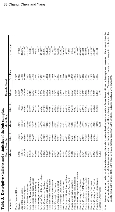
Table 3. Descriptive Statistics and t
-statistics of the Sub
-samples. Entire Sample Male Head Female Head Variabl e Mean Std Dev Mean Std Dev Mean Std Dev t-Statistic
Female Household Head
0.0987 0.2983 District 2.6985 1.9363 2.6875 1.9356 2.7989 1.9399 -5.7352 **
Age of the Male Spouse
42.8175 10.2649 42.9723 10.3251 41.4059 9.5856 16.1842 **
Age of the Female
Spouse 39.7020 9.5596 39.0617 9.1302 45.5440 11.2581 -58.4720 **
Male Decedent of Mainland
0.2281 0.4196 0.2196 0.4140 0.3054 0.4606 -18.7719 **
Male Never Moved from the House
0.6440 0.4788 0.6472 0.4779 0.6151 0.4866 6.6011 **
Male Moved within Same
District 0.0471 0.2120 0.0479 0.2136 0.0407 0.1976 3.6060 **
Male Moved within Same City
0.0809 0.2727 0.0808 0.2726 0.0819 0.2742 -0.3784
Male with High School Education
0.2584 0.4377 0.2534 0.4350 0.3044 0.4602 -1.1068 **
Male with College Educat
ion or above 0.4296 0.4950 0.4378 0.4961 0.3554 0.4786 17.1183 **
Male Working as an Employer
0.1062 0.3082 0.1143 0.3182 0.0329 0.178 41.3064 **
Male Working as Self Employed
0.1730 0.3783 0.1856 0.3888 0.0592 0.2361 49.4008 **
Male Employed in Private
Sector 0.4506 0.4975 0.4705 0.4991 0.2696 0.4438 44.6030 **
Male Employed in Public Sector
0.1879 0.3906 0.1890 0.3915 0.1784 0.3828 2.7642 **
Male Working in Own House
0.0933 0.2909 0.0992 0.2989 0.0402 0.1966 28.1620 **
Male Working in Own District
0.4237 0.4941 0.4416 0.4966 0.2607 0.4390 40.5861 **
Male Working in Other Districts
0.4110 0.4920 0.4281 0.4948 0.2548 0.435 39.1521 **
Female Decedent of Mainland
0.2185 0.4132 0.2052 0.4038 0.3402 0.4738 28.8376 **
Female Never Moved from the House
0.6320 0.4822 0.6355 0.4813 0.6015 0.4896 6.9372 **
Female Moved within Same District
0.0458 0.2090 0.0465 0.2105 0.0395 0.1949 3.5391 **
Female Moved within Same City
0.0805 0.2721 0.0803 0.2718 0.0827 0.2754 -0.8559
Female with High School Educati
on 0.3047 0.4603 0.3115 0.4631 0.2435 0.4292 15.6838 **
Female with College Education or above
0.3034 0.4597 0.2790 0.4485 0.5260 0.4993 -49.8635 **
Female Working as an Employer
0.0246 0.1551 0.0160 0.1253 0.1042 0.3055 -30.0928 **
Female Working as Self Em
ployed 0.0431 0.2032 0.0333 0.1795 0.1329 0.3394 -30.3667 **
Female Employed in Private Sector
0.2505 0.4333 0.2281 0.4196 0.4553 0.4980 -46.2094 **
Female Employed in Public Sector
0.1325 0.3390 0.1253 0.3311 0.1986 0.3990 -18.6320 **
Female Working in Own H
ouse 0.0375 0.1900 0.0343 0.1819 0.0674 0.2507 -13.5101 **
Female Working in Own District
0.2263 0.4184 0.2082 0.4060 0.3925 0.4883 -18.6320 **
Female Working in Other Districts
0.2158 0.4114 0.1898 0.3922 0.4537 0.4979 -13.5101 ** Number of Observations 11,191 10,086 1,105 Note:
Means and standard deviations of the entire sample, the male household head sub
-sample, and the female household head sub
-sample are presented. The t
-statistic is on the
differences between the means of the two sub
-samples
. Note that most of the variables are binary dummy variables. The mean of a dummy can be interpreted as the ratio of a
specific group in the sample. Refer to the paper for a more detailed discussion on the variables.
** Indicates significant level beyon
There is a higher rate of home businesses in the Western area; the ratio s for household head working at home are 17.65 percent (male) and 6.25 percent (female), much higher than the city average. The Western District also has the lowest ratios for residents to commute to work places outside of their own district. Higher proportions of households who work outside the city are found in the Eastern (51.13 percent, male) and Southern (57.25 percent, male) Districts; the ratios are relatively high for both male and female household heads. On the other hand, in Western, Northern and both Central Districts, the households mostly work in the same area that they live in; the rate is from 39 to 44 percent.
The empirical data was obtained from the 1990 Census of Population and Housing, Taipei, Taiwan. The Census’ data notes there are 670,626 households in the Taipei City area. The main purpose of this paper is the household’s location choice of self-owned residences. Therefore, military records, overseas residents, and foreigner data are all deleted from the data set. In terms of house ownership sources, only normally self-owned houses were selected; houses purchased from government housing projects, inherited, or rented were eliminated. In addition, single owner households (or for any reason the spouse is absent), vacant properties or mixed-use properties were also deleted.
The screened out data was further randomly sampled within each district, and missing values were also deleted. This results in a random sample of 11,191 observations, amounting to 6.75 percent of the total count from the population data. The sample reveals that 10,086 households or 90.1 percent are recorded to have a male household head, and 1,105 or 9.9 percent have a female household head.5
For simplicity, we make four assumptions for the empirical model. First, this paper does not consider the roles played by the parents of the decision-makers, their children, and other household members in the household decision-making process. The parental influence on housing choice is well documented in Asian societie s. If parents live in the same house with the couple, or if the house is a gift from the parents, then these parents may directly influence the housing location choice. This is the primary reason why we have removed the housing data pertaining to inherit ance and gifts from the model.
Second, we assume the impact of children on their parents’ housing choice
5
A large sample size is maintained in order to keep enough observations for the female headed household sub-sample. The SAS random sampling program is utilized to obtain the sample.
be embedded in or explained by the characteristics of the parents.
Children may impact a household’s housing location choice in many ways. A direct impact of such may come from any financial contribution the children may offer to their parents. However, this impact is not widespread and can be very limited.6 An indirect impact from the children can very well come from selection of schools. Families consider choosing the “elite school” area for their children in elementary and junior high schools. The public school fiscal allocation in Taiwan is based on the neighborhood and community population. However, we assume this consideration does not play a significant role in our study, since the areas are large enough to offer diversity of schooling within each area. We did not include children related variables in the data set.
Third, limited by the 1990 Census data, we have no current income variables and housing price information. We consider some available variables, e.g., employment and education status, as good proxies for the income of the household.
Lastly, we assume that households have complete information about the property markets of each alternative location. The choice of housing location is a rational and informed decision.
In order to analyze the decision of housing location choices, we choose explanatory variables reflecting the household’s head and spouse characteristics in seven categories: the gender of the household’s head, ages of the spouses, family origins, places of residence in the previous five years, educational attainments, occupational status, and places of work. The variables are introduced in details below:
1) The gender of household head 7. This is a dummy variable (1 =
female, and 0 = male). Males traditionally play the role of household heads, and may have a more significant influence on the housing decision. In the case where the household head is female, it may imply the female spouse is more respected. Moreover, the income level of such households may be
6
Family’s buying decision studies revealed that children do not have influence. However, there is a higher probability that the decision of a youth member that gives more financial contributions, or possesses a better product understanding, may be used, hence said youth plays a bigger role in the buying decision-making (Beatty and Talpade’s, 1994). Therefore, this paper focuses on housing instead of the ordinary products. Since the role played by children is minimal, this angle shall not be included in the discussions.
7
If the independent variables including both the dummy variables of household head and spouse sex into the model, then a collinear problem will be suffered. Hence we took the sex of the household head as the representative variable.
different from that of male household heads. Hence, the needs of the housing location environment may also differ. It is expected that there is a significant difference between the two types of households on the location choice.
2) Ages of Spouses. The age of the household head and his or her
spouse possibly implies different life cycles, household needs, income levels, and traditional ideology. Due to their high income and savings, they may opt for locations near the more expensive central city. Older couples are also more likely to be accustomed to the traditional ideology where the female spouses have less influence on family decisions.
3) Family Origins. We code two dummy variables for both husband
and wife to indicate if he or she is from a family originally registered from Mainland China. If the husband(wife) has a Mainland origin, Male
Decedent of Mainland (Female Decedent of Mainland) is set to one;
otherwise it is set to zero. Today’s Taiwan society is becoming more socially integrated. Is the place where the family originally registered becoming less distinct in housing location choice? This paper attempts to explore whether these variables are significant in the location selection behavior.
4) Place of Residence Five Years Ago. We created three dummy
variables for either the husband or wife. 1) If five years ago the husband (wife) lived in the same house, Male (Female) Never Moved Fro m the
House is equal to one. 2) if the husband (wife) lived in the same district but
not the same house, Male (Female) Moved within Same District is equal to one, and 3) if the husband (wife) lived in another district but the same city,
Male (Female) Moved within Same City is equal to one. Thus, the default
groups are those who moved from the outside of the city. These six variables can help to understand how the previous experience characteristic influence on the housing location choice. In addition, we also ask another question: whose previous living experiences have the stronger influence on the location choice; the husband’s or the wife’s?
5) Education Attainment: Two dummy variables are generated for
either the husbands or wife. 1) If the husband (wife) has only a high school education, Male (Female) with High School Education is set to one, and 2) If the husband has only a college education or above, Male (Female) with College Education or above is set to one. The default group is for those who only have middle school or lower education. There is a significant difference between the choices made by households having a low level of education and the choices made by those having middle or higher levels of education. The households with a background in higher education are expected to have higher utilities, e.g., higher quality living environment. Furthermore, does a spouse with higher education have a stronger
influence? Since this data set lacks income data, this variable could be used as a proxy for the income levels of the husband and wife.
6) Occupational status: Based on the Census data, we created four
dummy variables for the husband and wife. 1) If the husband (wife) is an employer, Male (Female) Working as Employer is one. 2) If the husband (wife) is an own-account worker, Male (Female) Working as Self-Employed is one. 3) If the husband (wife) is employed by a private company, Male
(Female) Employed in Private Sector is one, and 4) if the husband (wife) is
employed by the government, Male (Female) Employed in Public Sector is set to one. This leaves the default groups to be an unpaid family worker or people not working. Employers are expected to earn higher income than their employees do. Therefore, the employers have a stronger preference for locations with good environment and higher housing prices. We consider this variable as a proxy for income. Self-employed workers could work in their own homes. Moreover, they may be used to compare the economic status of the husband and wife, and which of the two plays a stronger role in location choice.
7) Place of work. The distance from home to workplace is the center
of location choice theory. We created three dummy variables for each spouse. 1) If the husband (wife) works at home, Male ( Female) Working in
Own Home is equal to one. 2) If the husband (wife) works not at home but
in the same district that they live in, Male (Female) Working in Own
District is equal to one, and 3) If the husband (wife) works in another
district rather than where they live, Male (Female) Working in Other
District is equal to one. These options leave people who work outside the
city to be the default comparison group. The closer the home is to the place of work, the more one saves on transportation costs. In addition to transportation cost savings, there are other actual conditions that may limit choice in the housing location choice decision. The considerations of the household to the two household members can also be compared.
The readers should bear in mind that all these above dummy variables are mutually exclusive within the same category.
We employ ordered-response Probit models that are suitable for the estimation of limited dependent variables with thresholds and discrete choices. The model is based on the assumption that the disturbance in the equation follows a specific distribution, e.g., a normal distribution. It is specified to directly estimate the probability of each of the choices being elected. Following the approach of Maddala (1983), the model can be described as:
where Xi is a vector of exogenous variables, including the characteristics of the spouses specified above; Y is the underlying location choice variable,
and µi is the residual, µi ~IN(0,1). The log-likelihood function can be
estimated. Estimates of the equation presented in the following section are computed using the SAS Probit procedure that utilizes the Newton-Raphson algorithm. The result presented in this work is estimated with the normal distribution. Note that the cumulative probability function is positively dependent on β that a positive coefficient results in an increasing (a decreasing) probability of contracting shorter (longer) term leases.
3.
Results and Analyses
The means and standard deviations of the entire sample, the male household head sub-sample, and the female household head sub-sample, are presented in Table 3. This table also demonstrates the t -statistical tests on the differences between the means of the two sub-samples. Note that most of the variables are binary dummy variables. The mean of a dummy variable can be interpreted as the ratio of a specific group in the sample. It is evident that the two sub-samples with either a male or female household head are strikingly different from each other. Nearly all variables are significantly different in means. The only two exceptions are Male
Moved within Same City and Female Moved within Same City within the
past five years. In general, the households in the female head sub-sample are located in the more expensive areas of the city than the other sub-sample, as reflected in the means of the District variables. The age of the male spouse is slightly lower, but the age of the female spouse is about five years higher than that of the sub-sample of the male head sub-sample. Among these households with a female household head, both spouses have been less mobile in the past five years. The female spouses tend to have better education attainment. The male (female) spouses have a higher(lower) ratio on high school education, but lower (higher) ratio of college education. These female spouses are also more active in the work force. For example, the ratio for them to be an employer is 10.42 percent relative to 1.60 percent of their counterparts’. On the other hand, the male spouses in these households show relatively weak employment positions. In terms of working locations, the female members are more likely to work at home, or within the same area or city. It indicates that chances for them to work outside of the area or city are considerably low. However, the male spouses in these same households tend to have a very high ratio of working outside of the city boundary. In summary, the reason why some households register a female household head is clearly evident. These households demonstrate the force in gender equality in modern Taiwan. The results from the ordered response Probit model are presented in Table 4. The log likelihood is highly significant for all three models. For each
sample the parameter estimates are tested using Wald Chi-Square tests. We discuss these results from the three samples separately below.
3.1 Entire Sample
For the entire sample, the significance of the characteristics of male spouses is very robust. The ages of male and female spouses both have negative coefficients, which indicates the low probabilities of older couples choosing less expensive locations. Older households are more likely to live in central areas (Central 1 and Central 2) and the more expensive Northern suburb. People with Mainland China origins also demonstrate the same preferences for locations.
In terms of household mobility, the more mobile the male spouse, the more likely he lives in an inexpensive area. The variable Male Never Moved from
the House (the male spouse who has not moved in the past five years)
shows a significant positive parameter estimate; i.e., the likelihood of selecting a less expensive area is high. The parameter estimates are also significantly positive for the other two variables (Male Moved within Same
District and Male Moved within Same City) in this category. Noticeably,
the parameter estimates for the female spouses, the variable Female Never
Moved from the House, show a significant negative parameter estimate; the
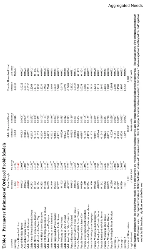
Table 4. Parameter Estimates of Ordered Probit Models Ent ire Sample
Male Household Head
Female Household Head
Variable Estimate Std Error Estimate Std Error Estimate Std Error Intercept -1.6991 0.0730 ** -1.8052 0.0816 ** -2.0045 0.2076 **
Female Household Head
0.0285
0.0148
*
Age of the Male Spouse
-0.0105 0.0008 ** -0.0083 0.0008 ** -0.0222 0.0025 **
Age of the Female Spouse
-0.0124 0.0008 ** -0.0154 0.0009 ** -0.0010 0.0022
Male Decedent of Mainland
-0.0410 0.0103 ** -0.0271 0.0109 ** -0.0550 0.0310
Male Never Moved from the House
0.2343 0.0256 ** 0.2415 0. 0273 ** 0.2268 0.0742 **
Male Moved within Same District
0.1902 0.0438 ** 0.1972 0.0460 ** 0.1710 0.1446
Male Moved within Same City
0.1124 0.0333 ** 0.1055 0.0352 ** 0.1956 0.1032
Male with High School Education
0.2428 0.0099 ** 0.2439 0.0105 ** 0.2234 0.0319 ** M
ale with College Education or above
0.4078 0.0116 ** 0.4069 0.0123 ** 0.3566 0.0378 **
Male Working as an Employer
0.4029 0.0270 ** 0.4433 0.0288 ** 0.2764 0.0919 **
Male Working as Self Employed
0.2349 0.0267 ** 0.2732 0.0286 ** 0.1565 0.0838
Male Employed in Pri
vate Sector 0.2033 0.0255 ** 0.2484 0.0273 ** 0.0137 0.0765
Male Employed in Public Sector
0.2757 0.0261 ** 0.3071 0.0279 ** 0.2401 0.0793 **
Male Working in Own House
-0.1005 0.0298 ** -0.0720 0.0335 * -0.0476 0.0901
Male Working in Own District
-0.0273 0.0275 0 .0023 0.0312 0.0496 0.0760
Male Working in Other Districts
-0.3632 0.0276 ** -0.3398 0.0313 ** -0.2489 0.0774 **
Female Decedent of Mainland
-0.0645 0.0103 ** -0.0458 0.0110 ** -0.1120 0.0311 **
Female Never Moved from the House
-0.0508 0.0254 * -0.0584 0.0271 -0 .0427 0.0735
Female Moved within Same District
0.0295 0.0442 0.0188 0.0464 0.0868 0.1463
Female Moved within Same City
0.0409 0.0332 0.0397 0.0351 0.0238 0.1024
Female with High School Education
0.1980 0.0099 ** 0.1970 0.0105 ** 0.2080 0.0336 ** Female with C
ollege Education or above
0.3724 0.0123 ** 0.3739 0.0132 ** 0.3710 0.0367 **
Female Working as an Employer
0.1870 0.0282 ** 0.1578 0.0338 ** 0.2826 0.0638 **
Female Working as Self Employed
0.0628 0.0241 ** 0.0491 0.0269 0.1251 0.0620 *
Female Employed in Private
Sector -0.0129 0.0206 -0.0346 0.0223 0.1319 0.0571 *
Female Employed in Public Sector
0.1242 0.0221 ** 0.1248 0.0240 ** 0.1640 0.0604 **
Female Working in Own House
0.0062 0.0240 0.0126 0.0257 0.1050 0.0755
Female Working in Own District
0.0369 0.0202 0.0355 0 .0218 0.1603 0.0628 **
Female Working in Other Districts
-0.2236 0.0212 ** -0.2026 0.0229 ** -0.1964 0.0632 ** Intercept 2 0.1982 0.0023 ** 0.1951 0.0024 ** 0.2305 0.0079 ** Intercept 3 0.5017 0.0033 ** 0.5069 0.0035 ** 0.4589 0.0105 ** Intercept 4 0.8559 0.0041 ** 0 .8520 0.0043 ** 0.8997 0.0133 ** Intercept 5 1.4194 0.0050 ** 1.4259 0.0052 ** 1.3765 0.0156 ** Number of Observations 11,191 10,086 1,105 Log Likelihood -18299.5062 -16489.6679 -1787.6671
Note:Parameter estimates from the ordered Probit models for the e
ntire sample, the male household head sub
-sample, and the female household head sub
-sample are presented. The standard errors of the estimates are tested with
Wald Chi
-square tests. The dependent variable is
District
, the location variable with six orde
red values. Refer to the paper for a more detailed discussion on the variables.
** Indicates significant level beyond 1%, and * significant
level at the 5%. Level and
The better the employment status of the male spouse (e.g., Male Working
as an Employer, with a parameter estimate of 0.4029), the more likely the
household lives in a less expensive suburban area. On the other hand, this effect is positive but not as strong for the female spouses. The variable,
Female Working as an Employer, only has a parameter estimate at 0.1870.
Furthermore, Female Working in Private Sector is insignificant. From the comparison of the effects on male and female oriented parameters, one can infer that the location decision is more significantly dependent on the employment status of the male spouse than the female. It could be an indication that the position of the wife is inferior to the husband’s. An alternative plausible explanation could also be the unobservable income level of the spouses.
The location of the work place is also an important determinant in the decision of the housing location. The male spouses working in another district in the same city are likely to have the household select and expensive district. A similar effect exists for the female spouse variable,
Female Working in Other Districts, but is less robust relative to the male
spouse variable.
In summary, the variables regarding the characteristics of the male spouses are significant overall; only one out of 18 variables is insignificant. However, five of the 14 variables for the female spouses are insignificant. Furthermore, the parameter estimate for the Female Household Head variable is significantly positive, indicating a higher likelihood for these households to be in less expensive areas.
3.2 Household with Male Head Sub-Sample
The same ordered response Probit model is applied to the male household head sub-sample. On the characteristics of the male spouses, the results are strikingly similar to that from the entire sample; parameter estimates have the same signs and similar values. However, seven of the variables pertaining to characteristics of the female spouses are insignificant. Two variables (Female Never Moved from the House, and Female Working as
Self-Employed) that are significant in the entire sample become
insignificant. The likelihood estimates for the variables, Female with High
School Education, Female with College Education or above, and Female Employed in Public Sector, are significant and have same signs as in the
entire sample. The variables, Female Decedent of Mainland, Female
Working as an Employer, and Female Working as an Employer are
3.3 Household with Female Head Sub-Sample
The results from the sub-sample of the female household head greatly differ from those from the other sub-sample. Several variables on male-spouse characteristics are found to be insignificant, including variables as Male
from Mainland, Male Moved within Same District, Male Moved within Same City, Male Working as Self Employed, Male Employed in Private Sector, Male Working in Own House, and Male Working in Own District.
The employment status, mobility, and the distance to the work place are less influential in the location decision of these households.
More attributes of female spouse characteristics, on the other hand, are found to be significant in this model. Both education attainment status variables remain robust parameters; the values of estimates are close to those in the other sub-sample and the entire sample. All four employment-related variables are significant. In terms of the distance to work places, the variable, Female Working in Own District, is found to have a significant positive parameter at 0.1603, in contrast to its insignificance in the other two samples. It indicates that the household is likely to be located in a less expensive area if female household head works within that district. The variable, Female Working in Other Districts, demonstrates a significant negative coefficient similar to those in the other two samples. However, three variables pertaining to mobility of the female spouse (Female Never
Moved from the House, Female Moved within Same District, and Female Moved within Same City) are insignificant.
Summing up the results from the three samples, one can argue that the housing location choice is more likely dependent upon the characteristics of the male spouse in the family than the female spouse’s. It is interesting to note that the female spouse characteristics are less influential in the households having a male household head; fewer such variables are statistically significant in the male household head sub-sample. If a household is registered to have a female household head, the decision making process changes. Among these households, the female spouse’s demands are given substantially more considerations than their counterparts in households with male household heads. Other binary location Probit models are also tested for each of the district.8 The results are similar to these presented above.
8 A binary dummy variable is formed for each location. Two sub-samples are tested for each of the district. Results are similar to what is reported here.
4.
Concluding Remarks
Using t-statistical tests and ordered response Probit models, this paper examines the aggregated needs of both spouses in a household, and delves into the housing location choices of households. In approximately 10 percent of the total households, female spouses are registered as the household heads in the Census survey. These female household heads demonstrate higher education and employment levels. Their implicit needs for housing location are more likely to be entertained than their counterparts in households with male heads. However, in households with a male household head, the female spouses’ characteristics are less likely to be significant in the housing location decision. Male spouses’ needs overwhelmingly impact the location choice. These households are seemingly more traditional than those lead by female household heads. Overall, these results indeed reflect a changing Taiwanese society where gender equality in households is gradually improving.
Further research in this area can be conducted to examine the changes on the location decision criteria over a period of time. Such studies will help to reveal whether the housing location choice process gradually becomes more democratic, and whether the female spouse's role becomes gradually more important. It can also verify the significance of improvement by combining characteristics of both spouses in the equation. Similar empirical tests can also be performed by introducing the income factor into the equation. In this paper we assume that income is implied in age and education of households.
In addition to the housing location studies, we raised the discussion on the aggregated housin g demands of both the husband and wife. This paper draws attention to the gender characteristics for the study of housing location choice. The results from this research will have an impact on the housing policies in Taiwan for some years to come.
References
Baber, K. M. and Katherine R. A. (1992). Women and Family: Feminist
Reconstructions, the Guilford Press.
Beatty, S. E. and Salil T. (1994). Adolescent Influence in Family Decision Making: A Replication with Extension, Journal of Consumer Research,.21, September, 332-341.
Bielby, W. T. and Denise D. B. (1992). I Will Follow Him - Family Ties, Gender- Role Beliefs, and Reluctance to Relocate for a Better Job, American
Camstra, R. (1996). Commuting and Gender in a Lifestyle Perspective, Urban
Studies, 33, 2, 283-300.
Chang, C. (1993). The Economic Analysis of the Family Choice Behavior,
Monographic Research Project of the National Science Council, pp. 1-11
(in Chinese).
Chen, Y. (1997). The Sequential Decision Models for Housing Choice,
Journal of Housing Studies, 5, 37-49 (in Chinese).
Cook, C. C. and Nancy M. R. (1984). Factors Influencing the Residential Location of Female Householders, Urban Affairs Quarterly, 20, 1, September, 78-96.
Fu, M. (1984). A Study of Housing Ownership and Housing Type Choice in
the Taipei Metropolis -- A Research of Logit Model, Unpublished Thesis,
Department of Urban Planning, Chung-hsing University (in Chinese). Gilroy, R. and Woods R. (1994). Housing Women, Routledge Press.
Heenan, D. and Anne M. G. (1997). Women, Public Housing and Inequality: A Northern Ireland Perspective, Housing Studies, 12, 2, 157-171.
Lin, C. (1990). Housing Needs and Tenure Choices under the Inverse Nested Multinomial-Logit Model, Academia Economic Papers, 18, 1, 137-158 (in Chinese).
Lin, C. (1994). The Associated Estimates of Housing Needs and Tenure Choice for Taiwan Area, Journal of National Chengchi University, No. 68 (in Chinese).
Lin, F., et al. (1996). Feminist Theories and Schools, Woman's Book Publishing, pp. 179-214. (in Chinese)
Liu, Y. (1996). Housing Choice - Changes of the Taipei City Households, Unpublished Thesis, Department of Land Economic, Chengchi University (in Chinese).
Maddala, G. S.(1983). Limited-Dependent and Qualitative Variables in
Econometrics, Cambridge University Press, pp. 13-78.
Munro, M., and Susan J. S. (1989). Gender and Housing: Broadening the Debate, Housing Studies, 4, 1, 3-17.
Samsinar, S.(1994). The Pattern of Role Structure in Family Decision Making in Malaysia, Journal of Asian Business, 10, .3, 31-48.
Smith, S. J. (1990). Income, Housing Wealth and Gender Inequality, Urban
Studies, 27, 1, 67-88.
Tu, Y. and Goldfinch J. (1996). A Two- Stage Housing Choice Forecasting Model, Urban Studies, 3, 517-537.
Williams, L. B. (1990). Development, Demography, and Family
Decision-Making: the Status of Women in Rural Java, Westview Press.
Yu, C. et al. (1996). The Sociology of the Feminist Point of View, Chuliu Publishing, 7-212 (in Chinese).