CAC and Packet Scheduling Using Token Bucket
for IEEE 802.16 Networks
Tzu-Chieh Tsai
Computer Science Department, National Chengchi University, Taipei, Taiwan, ROC [email protected]
Chi-Hong Jiang and Chuang-Yin Wang
Computer Science Department, National Chengchi University, Taipei, Taiwan, ROC {g9203, g9322}@cs.nccu.edu.tw
Abstract— The IEEE 802.16 standard was designed for Wireless Metropolitan Area Network (WMAN). The coverage of this new technology is expanded up to 50 km. IEEE 802.16 also has inherent QoS mechanism while the transmission rate can be up to 70Mbps. However, the main part of 802.16 – packet scheduling, was not defined and left as an open issue. In this paper, we present an uplink packet scheduling with call admission control (CAC) mechanism that is token bucket based. Also, a mathematical model of characterizing traffic flows is proposed. Simulations are carried out to validate our CAC algorithms and models. These results show that the delay requirements of rtPS flows are promised and the delay and loss can be predicted p r e c i s e l y b y u s i n g o u r m a t h e m a t i c a l m o d e l s .
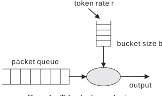
bucket size b
output token rate r
packet queue
Figure 1. Token bucket mechanism.
Index Terms—IEEE 802.16, WiMAX, Token Bucket,
Markov chain.
I. INTRODUCTION
Token bucket is a mechanism for controlling network traffic rate that injected to network. It works well for the “bursty” traffic. Two parameters are necessary in the token bucket mechanism: bucket size B and token rate r. Fig. 1 shows how it works. Each token represents a unit of bytes or a packet data unit. A packet is not allowed to be transmitted until it possesses a token. Therefore, over a period of time t, the maximum data volume to be sent will be
.
b
t
r
*
+
We adopt the token bucket mechanism to schedule the packets in 802.16 network environments.
802.16 is a new standard that aims at WMAN. The members of IEEE 802.16 had finished the original 802.16 standard in 2001[1], and 802.16a, 802.16c in 2002, 2003, respectively. In 2004, a new IEEE 802.16[2] standard known as 802.16 REVd was published, which is a revision of original 802.16, 802.16a, and 802.16c. In the original IEEE 802.16, transmission is restricted to Line-Of-Sight (LOS) but in the following standards, such as 802.16a and 802.16c, it can be Non-Line-Of-Sight (NLOS)[3]. The bit rate of 802.16 is 32-134 Mbps at
28MHz channelization. The transmission range of 802.16 is typically 4-6 miles.
The MAC part of 802.16 standard is not running under Carrier Sense Multiple Access with Collision Avoidance (CSMA/CA) that was adopted by 802.11 standard. 802.16 uses Time Division Duplex (TDD) or Frequency Division Duplex (FDD) to access the medium resource. Unlike 802.11, the first 802.16 standard has it inherent QoS support, it divides all traffic flows into four classes according to their application type and each class has different priority.
802.16 uses packet scheduling to achieve QoS support. However, there is no clear definition or implementation detail about the algorithm. The 802.16 standard only defines the QoS parameters and some simple principles. The other parts are open issues left to vendors.
The remainder of this paper is organized as follows. In Section II, we make a description about the IEEE 802.16 standard in detail. Section III includes some related work. Our call admission control and uplink packet scheduling models are proposed and explained in Section IV and Section V. In Section VI, we present the token rate estimation model. Simulation results are shown in Section VII. We conclude this paper in Section VIII.
II. IEEE802.16
In 802.16, the client-side node is called Subscriber Station (SS), and the server-side node is called Base Station (BS). And, there are four QoS classes defined in 802.16: Unsolicited Grant Service (UGS), real-time Polling Service (rtPS), non-real-time Polling Service (nrtPS), and Best Effort (BE). Table 1 shows these four
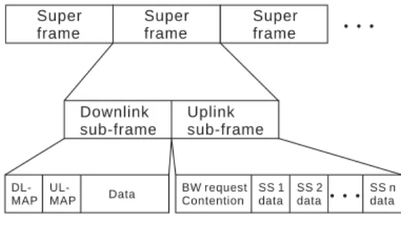
Super frame Super frame Super frame ˙˙˙ Downlink sub-frame Uplink sub-frame DL-MAP UL-MAP Data BW request Contention SS 1 data SS 2 data ˙˙˙ SS n data
Figure 3. 802.16 frame structure.
SS
BS
Traffic flows Traffic Policing Packet Queues Schedulor Call Admission Control Uplink Scheduling Create Connection Accept BW-Request Grant BW Send DataFigure 2 802.16 operation process.
QoS classes, where the upper class has higher priority than the lower ones. UGS packets are sent at a regular rate without the grant of each packet, so its delay requirement can be easily met. The nrtPS and BE traffic are non-real-time traffics, neither of them has delay requirements. Only rtPS flows, which is polled by BS in each frame, has the delay requirement.
Traffic flows in 802.16 are treated as connections. A traffic flow must establish connection with its BS before transmitting. The operation process of 802.16 is shown in Fig. 2[4][5]. The blocks drawn with dotted line in Fig. 2 are the parts undefined in 802.16. The traffic policing model can be simply achieved by applying token bucket mechanism[4].
The 802.16 standard divides transmission time into super frames and each super frame is divided into a downlink sub-frame and an uplink sub-frame. Downlink means the direction of transmission is from BS to SS, and the uplink means the direction is reversed. The downlink scheduling is considered simple because there is only one sender, BS. Hence we focus on the uplink scheduling.
After a BS accepts a new connection, BS will poll this new connection and give the SS the opportunities of sending its BW requests. This connection should send its bandwidth request (BW request) to the BS and wait for receiving BW grants (i.e. time slots for transmitting data) from BS. In this paper, we use the architecture in [4]: a connection sends its queue length as a BW request. The grants are the result of the uplink packet scheduling at BS and will be included in uplink MAP (UL-MAP) field in the downlink sub-frame. The 802.16 frame structure is depicted in Fig. 3.
The BW request contention period is designed for the lower priority classes, such as nrtPS and BE. The period lets these classes content for the opportunities of sending BW requests when system is too busy to poll all flows.
TABLE I. 802.16QOS CLASSES
Class Name Traffic Type Application UGS Real-time CBR Voice over IP rtPS Real-time VBR Real-time Video
nrtPS Non-real-time traffic FTP
Best Effort Non-real-time traffic HTTP
III. RELATED WORK
Kitti Wongthavarawat, and Aura Ganz [4] proposed an uplink packet scheduling mechanism with CAC. The overall bandwidth is allocated according to strict priority. The UGS class has the highest priority, and the BE class has the lowest priority. The class of higher priority will be served earlier than the lower one. The scheduling of UGS class is defined by the 802.16 standard. They applied earliest deadline first (EDF) service discipline to rtPS class. Packets with earliest deadline will be scheduled first. They applied weight fair queue (WFQ) service discipline to this service flow. They schedule nrtPS packets based on the weight of the connection (ratio between the connection’s nrtPS average data rate and total nrtPS average data rates). The remaining bandwidth is equally allocated to each BE connection. Arrival-service curve mechanism was adopted in this paper. They make use of it to predict the deadline of rtPS packets. They also proposed a CAC model. This paper is has high contribution and serves as our primary reference. Several researches have proposed similar packet scheduling methods. Xiaojun Xiao, Winston K.G. Seah, Chi Chung Ko, and Yong Huat Chew [6] proposes a scheduling with hybrid and hierarchical architecture. Their solution designed a primary scheduler in BS and a secondary scheduler in SS. The authors analyze the bounds of token rate and bucket size of a given traffic pattern. They presented some algorithms that are derivations of measurement-based traffic specification (MBTS). Our method is different from theirs. We find appropriate token rate by analyzing Markov Chain state and according to delay requirements of connections.
Mohammed Hawa, and David W. Petr [7] proposes a hybrid mechanism of weighted fair queue (WFQ) and priority queue. Allocating the BW-request contention size in uplink sub-frame is also discussed in this paper. The size of BW-request contention period was determined according to the amount of transmitting data.
Channel condition and some other factors were considered in [8]. In this paper, Reuven Cohen and Liran Katzir proposed a policy-based scheduling to maximize the bandwidth utilization. According to different load of synchronous, channel condition, and tolerated jitter, they proposed some different scenarios. Each scenario has its scheduler tasks.
Some research about characterizing a traffic flow by token bucket had been done such as [9]. Puqi Perry Tang and Tsung-Yuan Charles Tai use the measurement-based approaches to find appropriate token rate and bucket size. In [10], Tarkan Taralp, Michael Devetsikiotis, and
t t+f t+2f t+3f t+4f t+5f t+6f t+7f t+8f bi =3f di di =3f r fi r fi r fi r fi r fi r fi
Figure 4. A transmission of an rtPS connection that lasts for 6 frames. t t+f t+2f t+3f t+4f t+5f t+6f t+7f t+8f b /2i =3 d /fi r fi r fi r fi r fi r fi r fi b /2i =3 d /fi
Figure 5. Sharing bi packets in two frames.
Ioannis Lambadaris analyzed traffic flows with different types of arrival and infinite queue
IV. CALL ADMISSION CONTROL
Our CAC is based on the estimation of bandwidth usage of each traffic class, while the delay requirement of rtPS flows shall be met.
A. Naïve Estimation of Bandwidth
Assume that each connection is controlled by two token bucket parameters: token rate ri (bps) and bucket size bi (bits). And let f be the frame length, n be the session length of this connection. According to token bucket mechanism, the maximum data of this rtPS connection will be:
. (1) i
i
n
f
b
r
*
*
+
The bandwidth used at any frame can be estimated by dividing n*f in (1) as:
f
n
b
r
i i*
+
. (2)Using (2) as a metric of CAC, bandwidth will be enough for a connection at all time. However, for rtPS flows, delay requirement is not considered here. Therefore, a new parameter di as delay requirement of an rtPS flow is required. Using ri, bi and di, we shall develop a better estimation of bandwidth for a rtPS connection. B. An Example
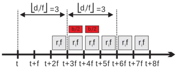
If an rtPS connection has a session from time t to t+6f, (which means n=6), the maximum size should be sent during each frame is shown in Fig. 4. The gray blocks represent the maximum size to be sent during that frame. And let delay requirement of this connection di=3*f.
Therefore, data arrived during frame [t, t+f] must be sent out during frame [t+2f, t+3f] at latest. We know that during a frame f, this connection will send data of rif+bi bits at most. If data generating rate is bigger than ri, bi is consuming. In the extreme case this connection may run out of bi at a certain frame. Assume that bi is totally
consumed during frame [t+2f, t+3f], as Fig. 4, this situation makes the maximum size should be sent out during frame[t+4f, t+5f] to be rif+bi bits. In Fig. 4, the bi
comes from the frame [t+2f, t+3f]. So only the frame [t+3f, t+4f] can share the bi bits of the frame [t+4f, t+5f]. Fig. 5 shows the result.
Hence, we estimate the data volume to be transmitted within a time frame as:
2
*
i ib
f
r
+
.Therefore, the bandwidth used within a time frame can be estimated as:
f
b
r
i i*
2
+
.C. Our Bandwidth Estimation
Let n and f still be the session duration and frame length respectively. When a traffic flow wants to establish a connection with BS, it sends parameters ri, and bi to the BS and waits for the responses from BS. An extra parameter, delay requirement di, will be sent by rtPS flows.
In order to meet delay requirement of rtPS packets, packets generated at time t must start to send after mi-1 frames after t, where
⎥
⎦
⎥
⎢
⎣
⎢
=
f
d
m
i i .If data rate is bigger than token rate, tokens in token bucket will be consumed. These bi bits can be shared by mi-1 frames before deadline.
Therefore, our estimation of the data volume in a time frame is:
1
−
+
i i im
d
f
r
.And, the bandwidth of the flow is estimated as:
f
m
d
r
i i i*
)
1
(
−
+
. (3)D. Call Admission Control
Let NrtPS be the number of rtPS connections, Bdemand be the bandwidth required by all rtPS connections, we can know that Bdemand can be calculated as:
∑
+
−
=
NrtPS i i i i demandf
m
d
r
B
)
*
)
1
(
(
. (4)In order to avoid starvation of some traffic classes, we set a threshold of bandwidth used for each class. They are: TUGS, TrtPS, TnrtPS and TBE, TUGS+TrtPS+TnrtPS+TBE≦Buplink, where Buplink is the total bandwidth of uplink. When the bandwidth occupied by a class is over its threshold, this class will have lower priority to the bandwidth resource.
The principle of our CAC algorithm is: First, system calculates the current available bandwidth. Second, for new incoming flows, system estimates the bandwidth it will take and the system will decide to grant this new flow or not. For rtPS flow, (3) is used to estimate its bandwidth; for the other three flows, ri , the token rate, will be used to estimate bandwidth. Our CAC algorithm is as follows:
Step 1. Calculate the remaining uplink bandwidth Bremain: Bremain=Buplink-BUGS-BrtPS-BnrtPS-BBE .
Step 2. Compare Bremain to the bandwidth requirement of the new connection. If there is enough capacity, the system accepts the incoming flow. If not, go to Step 3.
Step 3. Check if the lower-class flows has taken more bandwidth than its threshold (TrtPS, TnrtPS ,or TBE). If not, go to Step 4. If there is, the system will allocate the less time slots for these lower-class flows, then go to step 2.
Step 4. Check if higher-class flows has has taken more bandwidth than its threshold (TrtPS, TnrtPS ,or TBE). If not, go to Step 5. If there is, the system will choose some higher-class flows to degrade their ri. That is, “stealing” bandwidth from the upper-class flows.
Step 5. The system denies the incoming flow.
Stealing bandwidth from upper class may be an issue. Stealing bandwidth from BE and nrtPS flows is relatively simple. We can easily decrease the bandwidth used by them because of they are not real-time flows. To steal bandwidth from the other two real-time classes, we will choose some connections of these two classes and degrade their ri, e.g. make ri to be c․ri, where 0<c<1.
V. UPLINK PACKET SCHEDULING
In our uplink packet scheduling algorithm, We adopt Earliest Deadline First (EDF) mechanism proposed in [4]. There is a database that records the number of packets that need to be sent during each frame of every rtPS connection. Our uplink packet scheduling algorithm is described below.
Step 1. Apply the arrival-service curve and database mentioned in section III and [4] to the arriving packets during last frame of each rtPS connection. Calculate the deadlines of these packets by applying (3) and record them in the database.
Step 2. Grant all the UGS connections.
Step 3. Grant all the rtPS connections according to the rtPS database. Due to possible degradation of ri, we
should restrict the maximum grant size of a connection to (4).
Step 4. Assume that the total bandwidth requirements of nrtPS connections and BE connections are RnrtPS and RBE. We allocate Min(RnrtPS, TnrtPS) bandwidth to nrtPS
connections first. Then allocate Min(RBE, TBE) bandwidth to BE flows. The TnrtPS and TBE are threshold parameters mentioned in the last section.
Step 5. If there is remaining bandwidth, we check if RnrtPS>TnrtPS. If it is, nrtPS connections shall be granted with Min(remaining bandwidth, RnrtPS-TnrtPS) bandwidth. Also, If there is remainder bandwidth, we look if RBE> TBE. If it is, we grant Min(remainder bandwidth, RBE-BBE) to BE flows.
Step 6. If there is remaining bandwidth and there are some non-real-time connections that need BW-request contention opportunities, we allocate the remainder bandwidth to nrtPS and BE connections in order for BW-request contention periods.
VI. TOKEN RATE ESTIMATION MODEL
We have presented our CAC and uplink packet scheduling model in previous sections. Each connection in our scenario is controlled by token rate ri and bucket size, bi. The CAC and uplink packet scheduling are also based on the token bucket mechanism. However, not every traffic flow has a token rate parameter and bucket size parameter originally. In this section, we proposed a mathematical model to estimate the appropriate token rate of a traffic flow based on the queuing delay and loss rate requirements. We assume that the arrival of the traffic flow is Poisson. The cases of infinite queue and finite queue are analyzed. Both cases are single server and single queue ,because each traffic flow has its individual token rate and bucket size.
First, we show how to calculate the queuing delay when the queue size is infinite, when the token rate and bucket size are given. Second, we show how to calculate the queuing delay and loss rate when the queue size is finite, given the token rate and bucket size. At last, we show a simple search algorithm for finding the adaptive token rate of a traffic flow, given the queuing delay requirement, and the loss rate requirement.
A. Infinite Queue
Assume that there is a traffic flow with Poisson arrival, where λi is the mean arrival rate. ri and bi represents the
token rate and bucket size of this traffic flow.
Markov Chain is adopted to analyze the problem. We use discrete time Markov Chain. Each Markov Chain state is defined as State(t, p) where t represents the number of tokens stocked in the bucket and p represents the number of packets that stay in the queue. The time interval between two Markov Chain states is 1/ ri, that is, the time of generating a token. Hence we can find the probability P of n packets that arrive during the time interval 1/ri is:
!
)
(
n
e
n
P
n αα
⋅
−=
, where i ir
λ
α
=
.Because the time interval of our Markov Chain model is 1/ ri, there is at least one token generated when packets arrival. We take the State(bi, 0) as the beginning state of our Markov Chain. The transitions of State(bi, 0) are
shown in Fig. 6. The transitions of other states are all the similar. They are shown in Fig. 7. We take State(t, 0) as an example, which is a brief view of general case.
Assume state(t, p) is denoted by π(bi-t+p) and let
.
∑
∞ ==
2)
(
ii
P
M
We can list balance equations as follows.
)
1
(
)
0
(
)
0
(
π
π
⋅
M
=
P
⋅
. (5)And for n≧1, we have:
(
)
∑
− = ⋅ + + − + ⋅ = + ⋅ 1 0 ) 0 ( ) 1 ( ) 1 ( ) ( ) 0 ( ) ( n k P n k n P k M P n π π π . (6)Assume the Z-transform of Poisson and [π(0), π(1),
π(2)…] is Gp(z) and Gπ(z). Then apply Z-transform to (6)
and simplify it. And then using (5), we can get
)
(
)
1
(
)
0
(
)
0
(
)
(
z
G
z
z
P
z
G
P−
−
⋅
⋅
=
π
π . (7) And, we know: . (8)1
)
(
lim
1=
→G
z
z πUse (7) and (8), we find that: α
λ
π
−⋅
−
=
e
r
r
i i i)
0
(
, where i i r λ α = . (9)To find [π(0), π(1), π(2)…], we should make use of (5) to find π(1) first. After we know π(0) and π(1), we can utilize (6), π(0) and π(1) to find π(2). Continue this process we can find any π(n). The average queuing delay davg can be expressed as
M/D/1/ avg d bucket) in the token no P(see 0 bucket) in the token P(see d ⋅ + ⋅ = . (10) where dM/D/1 is the mean delay of a M/D/1 queue and
its value[8] is ) ( 2 2 i i i i i r r r
λ
λ
− − , given ri>λi. (11) And, . (12)∑
==
b-1 0 k i(k)
-1
bucket)
in the
token
no
P(see
π
Substitute dM/D/1 and P(see no token in the bucket) in (10) for (11) and (12) we can calculate the average delay of this flow if we give the parameters ri and bi
B. Finite Queue
Now we consider the case of finite queue with queue size q. This traffic flow has an extra parameter lq, which means its loss rate requirement. We still use Markov Chain to solve this case, but the number of states become limited, e.g. [π(0), π(1), …, π(bi+q-1)]. The transitions of states are the same as previous case except the last one. The transitions of the last state, State(0, q-1), are shown in Fig. 8
The balance equations are listed below.
(
1
(
0
)
(
1
)
)
(
1
)
(
0
)
)
0
(
⋅
−
P
−
P
=
π
⋅
P
π
. (13) For bi+q-2≧n≧1,(
)
(
)
∑
− = ⋅ + + − + ⋅ = − ⋅ 1 0 ) 0 ( ) 1 ( ) 1 ( ) ( ) 1 ( 1 ) ( n k P n k n P k P n π π π . (14)There is no clear mathematic solution for the equations above found by us, so a recursion method was introduced. We can find all π(n) very fast by means of computer. The average queuing delay can be expressed as
i q b k j Maxb k i avg r N q b k j Min j P k d i i
∑
+ −∑
= ∞ + − = ⎟ ⎟ ⎠ ⎞ ⎜ ⎜ ⎝ ⎛ ⎟⎟ ⎠ ⎞ ⎜⎜ ⎝ ⎛ − − + ⋅ = 1 0 ( 1,0) ) , ( ) ( ) (π
(15) t-1,0 t,0 t+1,0 P(0) P(2) P(2) P(0) ˙˙˙ P(3) P(4) P(5) ˙ ˙ ˙ t-2,0 P(2) P(0) t+2,0 P(0) P(2) P(3) P(4) P(5) ˙˙˙ ˙ ˙ ˙ P(1) P(1) P(1) P(1) P(1) b ,0i P(0)+P(1) b -1,0i b -2,0i P(0) P(2) P(2) P(0) P(3) P(4) P(5) ˙ ˙ ˙ ˙˙˙ P(1) P(1),where N=0.5 if j=0; N=0, otherwise. The average loss rate can be expressed as
i i q b k j b q k i avg r q b k j j P k l i i / ) ( ) ( ) ( 1 0 1
λ
π
∑
+ −∑
= ∞ + − + = ⎟ ⎟ ⎠ ⎞ ⎜ ⎜ ⎝ ⎛ ⎟⎟ ⎠ ⎞ ⎜⎜ ⎝ ⎛ − − + ⋅ = .(16) Figure 6. The transitions of State(bi, 0).After we solve [π(0), π(1), …, π(bi+q-1)], we can estimate the average queuing delay and average loss rate by equations above. Given a reasonable bi to the traffic
flow, we can use a simple search algorithm to find appropriate ri according to its dq and lq. We can put this Figure 7. The transitions of other Markov Chain states.
model in the SS. When a new traffic flow comes, SS can use this model so as to find appropriate ri, then the BS can schedule according this ri.
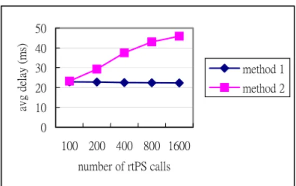
0 10 20 30 40 50 100 200 400 800 1600 number of rtPS calls avg de la y (m s) method 1 method 2
Figure 8. Avg. delay vs. number of rtPS calls. C. A Simple Search Algorithm
Assume that a Poisson arrival traffic flow with three parameters: mean arrival rate, λ i, queuing delay requirement, dreq, and loss rate requirement, lreq. If we give it a reasonable value of bucket size, bi, we can find the appropriate token rate, ri, for it by applying a simple search algorithm.
In the algorithm a factor a is can be assigned a value between 0 and 1 by the network operator. The factor a represents the degree of finding the appropriate token rate. The small a makes better result than large one but longer time for finding than larger a. In other words, the smaller the a, the closer to optimal value of token rate can be found. The algorithm works as follows:
Step 1. Set a reasonable initial value to ri. Check if the dreq and lreq are satisfied by applying (15) and (16). If satisfied, go to Step 2. Else go to Step 3.
Step 2. Set ri‧(1-a) to ri,new. Check if the dreq and lreq are satisfied by applying (15) and (16). If satisfied, set ri,new to ri and repeat this step. Else we take ri as the answer.
Step 3. Set ri‧(1+a) to ri,new. Check if the dreq and lreq are satisfied by applying (15) and (16). If not satisfied, set ri,new to ri and repeat this step. Else we take ri as the answer.
VII. SIMULATION RESULTS
We show the simulation results in this section. We validate our CAC and uplink packet scheduling first. Then the simulation results about our delay and loss rate calculation model are shown. Finally we briefly describe the multiplexing of two Poisson traffic flows.
0 5 10 15 20 100 200 400 800 1600 number of rtPS calls avg thr oughput (1 0 6 b ps ) UGS rtPS nrtPS BE
Figure 9. Avg. throughput of each class in method 1. A. CAC and Uplink Packet Scheduling
Two methods of CAC and uplink packet scheduling are compared here. Method 2 was proposed in [4] and method 1 was proposed by us.
0 5 10 15 20 25 30 100 200 400 800 1600 number of rtPS calls avg thr oughput (1 0 6 bps) UGS rtPS nrtPS BE
Figure 10. Avg. throughput of each class in method 2. The parameters of four classes are listed in Table II.
The begin time of each flow is Poisson distribution. All flows send data during each frame in full speed. Frame duration f is 1ms and simulation time is 150ms. The capacity of uplink is 37.5 Mbps. The queue size is infinite. The size of BW-request is 48 bits. rtPS connections send BW-requests on a per-frame basis. There are 100 flows of
UGS, nrtPS, and BE. Each connection has random beginning time and does not terminate. For the purpose of making the effect of CAC and uplink packet scheduling obvious, all connections send data in full speed.
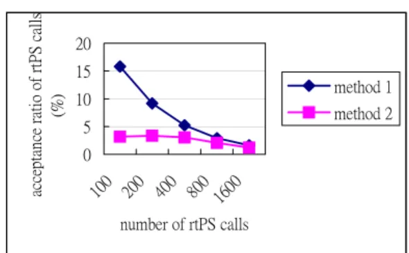
From Fig. 8 we can find that the average delay of rtPS used by our method is almost constant no matter how many rtPS calls exist. Fig. 9 and Fig. 10 show that the average throughput of each class by applying method 1 and method 2. From Figure 9, we can find that the average throughput of UGS connections is almost zero. That is starvation of UGS connections by applying method 2. However, there is no starvation when applying our method. Although we set a threshold parameter for each class, but the UGS did not reach its threshold when the numbers of rtPS connections are 200, 400, 800, and 1600. The reason is that too many rtPS connections occupy the bandwidth first. In Fig. 11, our method performs better in call acceptance ratio. Our method can receive more rtPS calls and guarantee their delay requirements.
TABLE II. SIMULATION PARAMETERS
ri (kbps)
bi (bits) dreq(ms) Packet
Size(bits) UGS 192 64 - 64 rtPS 640 15k 20 256 nrtPS 2000 15k - 256 Best Effort 512 8k - 128
0 50 100 150 200 250 64102 4 643072650000670000690000 token rate (bps) avg qu eu ing de la y (m s) Simulation Math
Figure 12. Avg. queuing delay vs token rate. 0 5 10 15 20 100 200 400 800 1600 number of rtPS calls accep ta nc e rat io o f rt PS cal ls (% ) method 1 method 2
Figure 11. Acceptance ratio of rtPS call vs number of rtPS calls. B. Delay and Loss Estimation
0 5 10 15 20 25 30 2000 00 3000 00 40000 0 5000 00 60000 0 70000 0 token rate (bps) av g de la y (m s) Simulation Math
Figure 13. Avg. delay vs token rate. Assume a traffic flow with Poisson arrival and its
simulation parameters are listed in Table III.The
simulation time is
(
ms. Fig. 12shows that the average queuing delay obtained by simulation and our calculation model given different token rates. We can see that the results of simulation and our calculation model are very close. This means our model is precise.
)
1 7 10 rate arrival mean − ×Then we show the result of finite queue case. The parameters of the simulation are all the same as infinite queue case except an extra parameter, queue size. The queue size is 5120 bits. Fig. 13 shows the average delay obtained by simulation and our calculation model given different token rates. Figure 14 shows the average loss rate obtained by simulation and our calculation model given different token rates. From them we can find both queuing delay and loss rate are very close between the simulation and our calculation model. The error percentage of queuing delay is 5.1% at most. This proves that our models are correct and precise.
C.Multiplexing
Assume there are n Poisson rtPS connections [c1, c2, …, cn] whose mean arrival rate are [λ1, λ2, …, λn]. If we give these n connections the same bucket size b and they have the same delay and loss requirements, which are d and l, we can find the appropriate token rates [r1, r2, …, rn] by applying the same simple search algorithm. Now we assume there is a Poisson rtPS connection csum whose mean arrival rate is λ1+λ2…+λn and has the same delay and loss requirement as those of n connections.
0 0.1 0.2 0.3 0.4 0.5 0.6 0.7 0.8 20000 0 3000 00 40000 0 50000 0 60000 0 70000 0 token rate (bps) avg lo ss r at e Simulation Math
Figure 14. Avg. loss rate vs token rate. The Poisson connection has the property that the mean
arrival rate of combining two connections with mean arrival rate λ1 andλ2 respectively is λ1+λ2. Hence we
can see csum as the aggregation of [c1, c2, …, cn]. If we also give this connection bucket size b and apply the simple search algorithm, we can find that the appropriate token rate of this flow is r1+r2+…+rn.
The results shown above means: if there are n Poisson rtPS connections whose delay and loss rate requirements are all the same and we give a reasonable value of bucket size, b, to them, the total token rate they need is the sum of their individual token rate, but the total bucket size they need is only b. Our bandwidth reservation for rtPS connections heavily depends on their bucket size. For the n traffic flows mentioned above,
1 − + ⎟ ⎠ ⎞ ⎜ ⎝ ⎛
∑
m b f r n i i need tobe reserved for these n flows instead of
∑
⎟ ⎠ ⎞ ⎜ ⎝ ⎛ − + n i i m b f r 1 , where f d m= .Less bandwidth can be reserved through multiplexing
TABLE III. SIMULATION PARAMETERS
Parameter Value
Mean Arrival Rate(kbps) 640 Bucket Size (bits) 5120 Packet Size (bits) 512 Queue Size (bits) 5120
when we make reservation for rtPS connections. VIII. CONCLUSION
In this paper we proposed a QoS-supported uplink packet scheduling and CAC mechanisms. Bandwidth needed by real-time flows can be correctly reserved while promising their delay requirements. We also proposed a model to convert Poisson traffic flow into token bucket-based connection. Multiplexing was also mentioned and evaluated in this paper. In the future, how to integrate CAC and uplink scheduling with token rate estimation model may be another issue we will concern.
REFERENCES
[1] IEEE, “IEEE Standard for Local and metropolitan area networks Part 16: Air Interface for Fixed Broadband Wireless Access Systems”, IEEE standard, December 2001.
[2] IEEE, “IEEE Standard for Local and metropolitan area networks Part 16: Air Interface for Fixed Broadband Wireless Access Systems”, IEEE standard, October 2004 [3] Carl Eklund, Roger B. Marks, Kenneth L. Stanwood and
Stanley Wang, “IEEE standard 802.16: A technical overview of the wirelessMAN air interface for broadband wireless access”, IEEE Communications Magazine, vol. 40, no. 6, June 2002, pp. 98 – 107
[4] Kitti Wongthavarawat, and Aura Ganz, “Packet scheduling for QoS support in IEEE 802.16 broadband wireless access systems”, International Journal of Communication
Systems, vol. 16, issue 1, February 2003, pp. 81-96.
[5] Dong-Hoon Cho, Jung-Hoon Song, Min-Su Kim, and Ki-Jun Han, “Performance Analysis of the IEEE 802.16 Wireless Metropolitan Area Network”, IEEE Computer
Society, DFMA’05, February 2005, pp. 130-137.
[6] Xiaojun XIAO, Winston K.G. SEAH, Chi Chung KO, and Yong Huat CHEW, “Upstream Resource Reservation and Scheduling Strategies for Hybrid Fiber/Coaxial Networks”,
APCC/OECC'99, vol. 2, October 1999, pp. 1163-1169
[7] Mohammed Hawa, and David W. Petr, “Quality of Service Scheduling in Cable and Broadband Wireless Access Systems”, Quality of Service, 2002. Tenth IEEE
International Workshop, May 2002, pp. 247-255
[8] Reuven Cohen and Liran Katzir, “A generic quantitative approach to the scheduling of synchronous packets in a shared medium wireless access network”, IEEE
INFOCOM 2004 - The Conference on Computer Communications, vol. 23, no. 1, March 2004, pp. 1674 –
1684
[9] Puqi Perry Tang and Tsung-Yuan Charles Tai, “Network traffic characterization using token bucket model”, IEEE
INFOCOM 1999 - The Conference on Computer Communications, no. 1, March 1999, pp. 51 – 62.
[10] Tarkan Taralp, Michael Devetsikiotis, and Ioannis Lambadaris, “Traffic Characterization for QoS Provisioning in High-Speed Networks”, IEEE Computer
Society, Thirty-First Annual Hawaii International
Conference on System Sciences-Volume 7, January 1998, pp. 485.
[11] Kleinrock L., “Queueing Systems. Volume I: Theory”, John Wiley, New York, 1975.
Tzu-Chieh Tsai was born in Tainan, Taiwan, R.O.C. He received his BS and MS degrees both in Electrical Engineering from National Taiwan University in 1988, and from University of Southern California in 1991, respectively. After that, he joined University of California, at Los Angeles in 1991. He got a PhD degree in Computer Science at UCLA in 1996.
His major research area includes IEEE 802.16, WLAN & QoS, mobile internet and QoS, pricing network, wireless sensor networks, wireless mesh networks, etc. Currently, he is an associate professor and chair in Computer Science Department at National Cheng-Chi University, Taipei, Taiwan.
Chi-Hong Jiang was born in Taipei, Taiwan. He receives his BS and MS degree in Computer Science Department at National Cheng-Chi University, Taipei, Taiwan at the year of 2003 and 2005, respectively. His main research interest is 802.16 MAC protocols and the integration of IEEE 802.16/802.11. He is now an software engineer at the Syscom group in Taipei.
Chuang-Yin Wang was born in Taipei, Taiwan. He is now a graduate student at Mobile Computing LAB1 in Computer Science department of National Cheng-Chi University. He receives BS degree in National Sun Yat-Sen University in the year of 2003. During his study toward the field, he has well developed the research interests upon 802.16 mesh networks. And some other research interests include the Mobile Ad-hoc networks, 802.16 MAC protocols.