ELSEVIER
Available online at www.sciencedirect.corn MATHEMATICAL AND
S(~IENClS ~DIRIEOTe
COMPUTER
MODELLING Mathematical and Computer Modelling 41 (2005) 501-522
www.elsevier.com/locate/mcm
Day-To-Day Vehicular Flow Dynamics in
Intelligent Transportation Network
H S U N - J U N G C H O * A N D I V I I N G - C H O R N G H W A N C Department of Transportation Technology and Management National Chiao Tung University, Hsinchu, Taiwan, Republic of China
h j cho©cc, n c t u . e d u . "tw
(Received April 2003; revised and accepted March 2004)
AbstractmIn this paper, a flow evolution model is developed by using the dynamical system approach for a vehicular network equipped with predicted travel information. The concerned sys- tem variables, path flow, and predicted minimal travel time of an origin-destination (OD) pair, are measured on the peak-hour-average base for each day. The time change rates of these two variables are formulated as a system of ordinary differential equations under the assumption of daily learning and adaptive processes for commuters. By incorporating the total perceived travel time loss (or saving) into the proposed models, time change rates of path flows are generated with a flow-related manner to prevent path flow dynamics from being insensible to traffic congestion which had been formulated in the existing studies. Heterogeneous models with various user adjusting sensitivities and predicted travel information are also presented. Equilibrium solutions of the proposed network dynamics satisfy the Wardrop user equilibria and are proved to be asymptotically stable by using the stability theorem of Lyapunov. The issue of existence and uniqueness of solutions is proved both on the lemma of Lipschitz condition and the fundamental theorem of ordinary differential equations. In addition, some simple examples are demonstrated to show the asymptotic behaviors of the proposed models numerically. (~) 2005 Elsevier Ltd. All rights reserved.
Keywords--Day-to-day network dynamics, Nonlinear dynamical system, Lyapunov function, Dy- namic traffic assignment.
N O M E N C L A T U R E t W P A P~
time index; unit: day
the full set of OD pairs with 17d OD pairs
the full set of paths w i t h / 5 paths the full set of links with .4 links the set of paths connecting OD pair w with P~ paths
the nonnegative peak-flow of path p at day t; unit: vehicle/hour
ht~ the sum of h~, Vp E Pw; unit: vehicle/hour
h t the full vector of path flows at day t
f t the nonnegative peak volume of link a at day t, i t = ~-~p ~aph~, where gay = 1 if link a belongs to path p, otherwise Sap = 0; unit: vehicle/hour
This research was supported in part by the Ministry of Education of Taiwan, R.O.C. under Crant EX-91-E-FA06- 4-4 and in part by the National Science Council of Taiwan, R.O.C. under Grant NSC-91-2211-E-009-050. *Author to whom all correspondence should be addressed.
0895-7177/05/$ - see front matter (~) 2005 Elsevier Ltd. All rights reserved. doi" l O.l O16 /j.mcm.2004.03.005
502 H.-J. CHO AND M.-C. HWANG
c~(/~)
¢
e t
the capacity of link a; unit: vehicle/hour
the unit average travel time on link a at day t, a smooth and strict monotone function of f~; unit: hour
the unit average travel time on path p at day t, without considering node travel time,
C t -~- ~-~(~apCa(f~a); unit: hour
a
t h e unit average travel time on OD pair w at day t predicted and provided by ATIS; unit: hour the full vector of c~w at day t
D~
~ p
X t
the travel d e m a n d of OD pair w over whole time period of interest; unit: vehicle/hour
the positive and path:specific parameter to denote the propensity of path flow dynamics; unit: vehicle/hour 2
the positive and OD-specific p a r a m e t e r to d e n o t e the sensitivity of predicted travel time dynamics; unit: hour2/vehicle
the ordinary derivative of x with respect to t
the transpose of vector (or ma- trix) x
1. I N T R O D U C T I O N
The ability to predict how the information prepared by advanced traveler information sys- tems (ATIS) influences the time trajectory of network flows is essential in the era of intelligent transportation systems (ITS). By providing road users with travel information and so allowing them to make better travel decisions, ATIS promises to enhance the utilization of existing trans- portation infrastructure and, consequently, to mitigate traffic congestion. The focus of this paper is to develop an analytical approach capturing the effects of travel information on network flow evolutions, especially the day-to-day interactions among system variables, network performances, and travel information. Network flow dynamics had been studied analytically [1-6] or simulation- oriented [7-15]. Some other researchers were concerned about formulations and solution methods of dynamic traffic assignment problem to compute the flow pattern under the conditions of sys- tem optimum [16-17], dynamic user equilibrium [18], or dynamic user optimum [19-21]. These studies did not simulate the evolutions of network flows but only a unique flow solution following some optimal criteria.
Conversely, the flow evolution model is able to capture the transition states of the system and finally approaches to steady state [22] if the system is well-behaved with a long enough evolution time. They are classified into two broad categories according to the time scales of system adjustment, the fluctuations of the system variables within each single day (intraday dynamics) and between subsequent "days" or more generally observation periods of similar characteristics (interday dynamics). Chang and Mahmassani's serial experiments [7-10] on route choice behavior of commuters had indicated that the learning and adaptive process of route choice may take weeks, partly because of the dynamic feedbacks from the traffic system, and, indeed, it can be lengthened by complex switching that resulted from the provision of better information. Friesz et al. [4] addressed Mahmassani's design theoretically by introducing a tatonnement process to model the transition of disequilibria from one state to another. Day-to-day dynamic models are particularly useful in capturing traffic patterns when perturbations of the traffic system create disequilibria that might adjust forward equilibria. If the duration of disruption or the time it takes for the system to reach equilibrium are such that the system stays longer in a nonequilibrium state rather than in an equilibrium one, it is important to catch the interday transition process of traffic diversion. Issues about interday transformation of peak-period commuter trips are examined in this research. A formulation of path flow alteration is presented though it is partly similar to Friesz et al. [4] but with new conceptual and mathematical refinements to offer a congestion-sensitive evolution behavior of network flows.
To sum up, the purpose of this paper is to develop an analytical approach capable of both modeling the interacted relationships between the aggregate user behaviors and ATIS informa- tion provision and characterizing the theoretical issues of the existence, uniqueness, and stability
Vehicular Flow Dynamics 503 for the proposed model with a thoroughly mathematical foundation. The achievements in the paper have never been reached before especially in a multiclass users scenario. As pointed out by Friesz et al. [23,24], the application of the proposed model mainly concentrates on the dy- namic network design problem. The dynamic network design problem is to determine a tempo- ral management (or control) plan which recognizes that perturbations generated from the new management (or control) treatments bring about disequilibria which adjust toward equilibrium. Therefore, a model of this type describes the time evolution of system states in a disequilib- rium adjustment framework and forms the basic feasible solutions of the dynamic network design problem.
The remainder of the paper is organized as follows. In the next section, we briefly mention the assumptions common throughout the paper. The major developments for network dynamics are described in Section 3. The proof of existence, uniqueness, and stability of proposed models is provided in Section 4. Numerical examples are demonstrated in Section 5, and the conclusions of this research are outlined in Section 6.
2. A S S U M P T I O N S
The basic assumption in the paper is the dally learning and adaptive processes of how system behaviors interact with the travel information predicted and provided by ATIS. Travel infor- mation about the upcoming day's travel time from origin to destination is provided with users and compared with the actual travel time experienced by all path users. Then, travelers who experienced travel time less than predicted travel time should have encountered a (pseudo) travel time saving. On the other hand, users who experienced travel time that is more than the pre- dicted travel time encounter a (pseudo) travel time loss. These deviations result in the path flows adjustments of the next day. Each link cost function is assumed to be a smooth and strict monotone function of link flow and is used to estimate the actual travel time for all paths. In addition, travel demand is presumably fixed in this study, without the loss of generality, under the assumption of no structural changes from competing transportation facilities over the whole period of interest. The authors are concerned that the variations of path flow and path travel time are much more sensitive than that of the OD demand if the travel information provided by ATIS is the only perturbation of transportation system. Therefore, by recording actual traffic volumes, ATIS evaluates the difference between the fixed travel demand and the sum of the path flows for each OD pair. In order to reflect the relative scarcity (or surplus) of transportation facilities, it is assumed that the predicted travel time of an OD pair adjusts accordingly as the difference between the fixed travel demand and the sum of the corresponding path flows is de- tected. Moreover, it is assumed also that travel demands of all OD pairs do not jointly violate any capacity constraints of all the links.
Some notation (see Nomenclature) based on the typical equilibrium models of commuter route choice are employed and augmented to meet our concerns. In particular, we take all vectors to be column vectors. Vectors and matrices are expressed in boldface.
3. M O D E L I N G N E T W O R K D Y N A M I C S
The contents of this section are distributed into two parts. The first is path flow dynamics that interact with ATIS, which are formulated in Section 3.1. The second is travel time evolutions of OD pairs that are predicted by ATIS, which are analyzed in Section 3.2. The whole network dynamics is a combination of these two components.
3.1. P a t h F l o w D y n a m i c s w i t h ATIS I n f o r m a t i o n
The basic behavioral assumption of least travel time seeking has been mentioned in Section 2. Before giving a mathematical relationship between path flow dynamics and this supposition, we
504 H.-J. CHo AND M.-C. HWANG
define the value of total perceived travel time loss (or saving) for path p E Pw at day t as t
PTTLp,~ - hp (c[ - c~).
O)
The perceived travel time loss (or saving) is measured by multiplying path flow with the difference between users' average experienced travel time for a path estimated by link cost functions and the predicted travel time provided by ATIS for the corresponding OD pair. This quantity can be viewed as an estimation of the total travel time loss (or saving) perceived by travelers driving path p at day t. The meaning of positive (negative) PTTL~,~ is that the average path travel time the users actually underwent is greater (less) than the travel time predicted by ATIS. Travelers might be motivated to change their route due to this difference. Alternatively, PTTL~,~ can be denoted as a measurement of path performance for the previous time point that results in the consequent shift of path flow at next time point. In addition, the congestion effect is embedded in PTTLp, w t implicitly by including the current state of path flow. It means that the values of PTTL~, w will be different at various congestion levels even under the condition that the difference between the average path travel time experienced by the users and the travel time predicted by ATIS is equal. The predicted travel time of OD pair w at day t, c~, is updated by another dynamic process that will be presented in Section 3.2. To continue our development, it is useful to postulate that future path flow is established through the tuning of the present state at a rate proportional to the value of PTTL~,~. That is,
where and h t + A t _ t p hp - ap (PTTL~,~) At,
(2)
O < a p < inf ( 1 ) , _ , c~ c~ (3a) cp cw~>OE
(- op pPTTLL ) < ko- E oph;,
(ab)
wE W V pEP~,, "¢ pEP
for all OD pair w E W, p e Pw, a e A, at day t. Inequalities (3a) and (3b) ensure to avoid non- feasibilities of nonnegative flow and link capacity constraints. It is obvious that inequalities (3a) and (3b) are naturally satisfied if ap is carefully calibrated from the empirical data. By taking
the limit of (2) as At approaches to zero and substituting (1) into (2), our path flow dynamics follow immediately as
=
% ( 4 - 4 ) ,
(4)
for all OD pair w E W, p E P~, at day t. The physical meaning of (4) is that the time change rate of the flow for path p at day t is equal to the negative product of the propensity of path flow shift and the value of PTTL~,~.
3.2. Travel Time Dynamics Predicted by ATIS
To forward the network traffic to a steady status is the major intent of ATIS. This goal is realized by successfully capturing travel time dynamics and delivering information to users. In this section, we will focus on the formulation of predicted travel time dynamics. To start the task, we first define the excess travel demand of an OD pair w at day t as
ETD~ - D~ - h~, (5)
where D~ denotes the time-invariant travel demand of an OD pair w over whole time period of interest. ETD~ is considered to be the difference between the travel demand and the sum of the corresponding path flows for an OD pair as denoted in [4] and [23]. Positive (negative) excess
Vehicular Flow Dynamics 505 travel demand means t h a t the rate at which users desire to depart from an origin to a destination is greater t h a n (less t h a n or equal to) t h a t where such movements are actually occurring. Then, predicted travel time is adjusted due to this deviation. Consequently, the predicted travel time dynamics for all OD pairs w C W at day t can be written as
c t + A t
- c~ + fl~
t
(D~
- h~) At,
t
(6)
where
0 < fl~ < min inf c ~ - c~
,
inf - c~(7)
[V(D~-h~<O) -- h~ V(D~-h~>O) h~ '
if we further suppose t h a t the travel time prediction of the next time point for an OD pair is transformed from the current status at a rate scaled to ETDt~. Inequality (7) guarantees t h a t all predicted travel times stay in the feasible region without greater t h a n ~ , the travel time at maximal flow, or less t h a n Z~, the travel time at free flow, for OD pair w. Then, we define
"cw= min ( ~ a 6ajCa(fa=O)
)
j
E
P
~
(Ta)
and
"c~=_max(~6~dca(fa=ka)).j~p.~
(7b)After taking the limit of (6), the predicted travel time dynamics can be written in differential form as
• t
dc~
c~ = dt =/%, (D~
-ht~) ,
(8)for all OD pairs w E W, at day t. Equation (8) reveals t h a t the time change rate of the predicted travel time for OD pair w at day t is equal to the product of the sensitivity of predicted travel time dynamics and ETD t . The whole version of network dynamics under operations of ATIS is accomplished as hl = hl ( 4 - 4 ) ,
Cw'~ = flw (Dw - h~)
o,-o,i'fE
E
(9)
0 < a p < P w>O w E W p E P w p E P c¢~ p--cw<O tO<flw < m i n ~ lV(D~'-h~ <0) inf w _~-~ , inf , V(D~-hi>0)
\Dw
- h~for all OD pairs w E W, p E P~, a E A, at day t. 3.3. M u l t i c l a s s U s e r s M o d e l
In this section, road users are classified into n subgroups to consider the effects of heterogeneous adjustments due to the various sensitivities of multiclass users on path flow dynamics. T h a t is to say, the parameter ap in (4) is not only path-specific but also user-specific. Consequently, there are n path flow dynamics for path
p E Pw,
at day t and (4) is augmented ash~p
dh~p
t
= = ( 4 - 4 ) , (lo)
for all OD pair
w E W, p E Pw
, i = 1 , 2 , . . . , n , at day t. The physical meaning of (10) is t h a t the time change rate of the flow for user class i using path p, at day t is equal to the506 H.-J. CHO AND M.-C. HWANG
negative p r o d u c t of the propensity of path flow shift for user class i and the value of perceived travel time loss (saving) for user class i, PTTL~p,~. If we further suppose t h a t there are two options for ATIS to provide predicted OD travel time, i.e., a homogeneous forecast for all users or individual predictions according to multiclass users, the predicted OD travel time dynamics should be reformulated as .~ dc~ c~ = d--t- = fl~ (D~ - ht~) (11)
or
= - h L ) (12)ciw = dt
for all OD pairs w C W, i = 1 , 2 , . . . ,n, at day t, respectively. In (11), the definition of ht~ is the same as mentioned before b u t calculated in a different way and expressed as
pePs, i
All components in (12) are reindexed from (8) by adding a subscript i for the corresponding user class in particular with
pE P~
Equation (12) tells us t h a t the time change rate of the predicted travel time for user class i traveling on OD pair w, at day t is equal to the product of the sensitivity of predicted travel time dynamics of user class i and the value of excess travel demand of user class i, E T D ~ . Now, the multiclass users dynamical systems for all OD pairs w E W, p E P~, i = 1, 2 . . . . , n, at day t are proposed as ~f,-~>o
.t
and E E E(- ~PTTL~,~) < ko ~ ~h~,
5 t _ t w E W iEN PEPw p E P t t i E N ap~c~<O 0 < f l w < m i n ~ inf( c ~ -ct~)
(c~----~----ct~} [V(D,.-h~<O) ~ 'v (D~--h~>0) inf -- h~ ] (15)for the case of providing a uniform prediction of OD travel time by ATIS and as
0 ~ sap <
t t
h~p - a i p hip (cp t • t -- fliw ( D i ~ _ hiw ) t ciwinf
<
1
),
E E E ( _ S a p ~ i p P T T L i v , w ) <__ ka __ E Saphip ( 1 6 ) cp cw> p -- iw w 6 W i E N PEPw p 6 P t t i 6 N Cp--C w ~00 < ~iw < min inf c ~ - - ~ t , inf - clw t
[ v ( D , ~ - h : ~ < 0 ) -- ~ v ( o , . ~ - h ~ , . > 0 ) - - F L '
for the case of individually supplying user-definite OD travel time, respectively.
Empirically, it is easy to be accomplished for such a hybrid system by providing a multiaccess information inquiry system. However, we are concerned about the asymptotic behavior of the steady state and whether it is in complete accord with the well-known Wardrop's user equilibrium. These topics are the major components in Section 4.
Vehicular Flow D y n a m i c s 507
4. E X I S T E N C E , U N I Q U E N E S S , A N D S T A B I L I T Y
A dynamical system is able to demonstrate the future states unambiguously when the evolution rules and initial situations are specified. The analysis of stability guides us to find out the network dynamics of where to go and when to be tranquil after perturbations are stirred up. In this section, we briefly illustrate the issue of existence and uniqueness of the proposed uniform-user model, i.e., (9), by the fundamental theorem of ordinary differential equations in Section 4.1. The steady state of (9) is analyzed to be in agreement with Wardrop's user equilibrium in Section 4.2, followed by the proof of the associated stability theorems using Lyapunov's direct method in Section 4.3. For the paxt of a multiclass model, brief statements based on the results of uniform-user model are provided in the latter part of these three sections. Time indices, day t, and inequalities (3) and (7) are omitted for conciseness in the subsequent sections, then, (9) is rewritten as
hp = - a p h p (cp - c~),
d~ = 3~ (D~ - hw).
(17)
4.1. Existence and Uniqueness
A dynamical system is a way of describing the time passage of all the points for a given space E. Mathematically, the space E might be a Euclidean space, R, or a subset of R. For the network dynamics mentioned in Section 3, the set of possible nonnegative path flows and predicted travel time is clearly a convex subset of RP+ +W, denoted as S even the constraints of path capacity are added. We have the following theorem in [26].
THEOREM 1. Suppose that G E CI(E) and that G(x) satisfies the global Lipschitz condition,
l a ( x ) - a ( y ) l < L l x - y l ,
(18)
for aIl x, y E E. Then, for x0 E R ~ the initial value problem,
± = G ( x ) , with x(0) = x0,
(19)
has a unique solution x(t) defined, for all t C R. The existence and uniqueness of (17) can be claimed if the G(x) in (17) C C 1 (RP+ +w) and satisfies the global Lipschitz condition.
The assumptions of the smooth and strict monotone function of link travel time ensure that the G(x) in (17) is CI(RP++W). Then, the proof of the global Lipsehitz of G(x) is given by the following lemma.
For convenience, G : S -* RP+ +W in (17) is reindexed as f g~ (W,c') = - ~ j h j (cj - c~), W e W, G (h',c')
l
gj (h', c') = #~ [D~ - h~], V ~ e W, j e { 1 , 2 , . . . , P } if path j E P~, j E{I+P,2+P,...,w+P},
(20)
and the normP+W
lyl = ~
Jy~l
/----1is used Vy E R~ +W. Now, we give the lemma of the Lipschitz condition for (20) and prove it. LEMMA.
stant,
C(h', c') defined in (20) satisfies the global Lipschitz condition with a Lipschitz con-
508 H.-J. CHO AND M.-C. HWANO where
: =
( ( (
0+
Lp
I<j<P t /eP:
Oh/ h+:Xj]
(21) sup a j h j ~ , sup ~ j h 3 .j,t#j j
PROOF. From the assumptions and definitions of the link cost function mentioned in previous sections, the G ( h ! , c ') in (20) is obviously continuously differentiable on S. Let u = x - y
' ( z, c~). Since convexity of S, and y, x are two given points in S, i.e., y ' = (hy,c~) and x ! = h !
the points v = y + bu are also in S, for all 0 < b < 1. Defining the function H : [0, 1] -o R p+W by
H (b) = G ( v ) , (22)
and by the chain rule, we have
P+W P+w
P+w P+w
dH (b) _ Y"2. ~
Ogi (v) dvt = ~ . ~
Og i (v) (x, _ y~),
db Or, db . - - - . - - . 0~,
j = l I=1 j = l I=1
and hence,
dH(b)
P+wP+W
0gj(v)dvt I P+WP+w Ogj
(v)- - x - - < Z E
j = l t=lor,
d b : E E
j = l t=lo~, I~-~,l.
(23)There are three conditions in (23) that keep ~ Ovt from vanishing for the path flow dynamics,
I !
i.e.,
Ygj, 1 <_j <_/5.
If we let v ' = (h~,%), they areogj(v)
0vl
= "j (cj - c=) + h j G )
I (
°~J\l
,
if l = y and 1 < l < P,
I Ogj
(v)
0cj
Ovt
= ajhjff-~l ,
if l 7~ j, path l overlaps partly with path j and 1 < l < / 5 ,Ogj(v) =[ajhjl,
V I + / 5 < I < P + W ,l----P+w, j c P = .
Ovt
(24)
The upper bound of I O-~tg in condition (24) can be decided by Ovt
sup ~ + h , _ ~ - - ~ , s u p ( ~ j h j ) .
(27)
l_<j<P I, de P~,
We know that
hp
and c= are bounded globally by constraints (3a), (3b), (7), (7a) and (7b). Hence, (25) is also bounded as the boundary conditions of (3a), (3b), (7), (Ta) and (7b) take place. That is to say, the upper bound of ~ Ovt in condition (24) is shown asLp = max o9~ = max sup + 7 = - 7 = ) + h, ohj h . - z , ] ]
I < j < P OVt I<_j<P [ j 6 . P ~
o+
(
)}
sup (+X, oh~ h,=x,]' sup +Xj
,
j,lCj
j
(26)
where
Vehicular Flow Dynamics 509
By similar treatments, there is only one condition that °gA~)l, Vgj a n d / 5 + 1 < j < /5 + W Ov~ -- -- in (23) is not equal to zero. It can be expressed as
%
Ov~
(v) I
= fl~' V 1 < l </5, if path l E P~. (28) The results of (27) and (28) lead us to setL
= max ~max {fl~ } ,L,;
(Vw
(29)
)
and hence,
" - - ' ~ <- E
P+WP+W ~ ]
j = l /=1= }-]
}-~P+~P+~ 0gj(v)
Ovl
j = l l = lNow, from the relation G(x) - G(y) = H(1)
f~ IH'(z)l dz
< n i x - Yl. Thus, G(h', c') in (20) satisfies the global Lipschitz condition and the corresponding Lipschitz constant L can be determined by (29). After proving the above lemma, the global existence and uniqueness of (17) is standard and we refer readers to [26] for a proof of the fundamental global theorem.For the cases of multiclass users, (20) is amplified as
G ( h , , c , ) _ f gj(h',ct)=-oiphip(Cp-Cw),
V w , p e P w ,
j=P(i-1)+p,
(30)
gj (h', c') = /3,o [D~o - h~,] ,
V w E W,
j = nP + w,
and { g j (h', c') =-aivhip (Cp - ci,o) ,
G(h', c') =I dvl
p+w
[ x l - y d _ < L E I x l - Y l l = L I x - Y l l = l-
H(O) =
f~o
H'(z) dz,
we find that IG(x) - G(y)] <where i = 1, 2 , . . . , n to fit (15) and (16), respectively• The dimension of G(h', c') and (h', c') in (30) are the same and denoted as
nP+IZV
and in (31) as n ( P + Pit). By the similar treatments, condition (24) for path flow dynamics with 1 < j _< n P is modified asogj (v),
Ogj
(v)
Ovl
ogj (v)
Ovl andI Ogj
(v)
I
%
(v)
I Ogj
(v)
Ovl h "Ocp~
cOe p = OLiphip-o-'~e z ,= [aiph~p[,
•Ocp "~
COCp ~- o Q p h i p - ~ e z ,= la~p%l,
V l e [1,n/5],i f l = P ( i - 1 ) + p ,
v l
[1, up],
i f l # P ( i - 1 ) + p a n d l = P ( e - 1 ) + z ,
V l e [ I + n P , n P + W ] ,
p e P s ,
if I = n/5 + w, Y l E [ 1 , n P ] , i f l = t h ( i - 1 ) + p , vz i f / # P ( i - 1) + p and l ----/5(e- 1) + z,Vle[l+nP, nP+nW], pePs,
i f / = r i P + I ~ ( i - 1) + w , (32)(33)
V w , p ~ P ~ ,
j = P ( i - 1 ) + p ,
(31)
V w E W ,
j = n P + ¢ V ( i - 1 ) + w ,
510 H . - J . C H O AND M . - C . HWANG
for the two cases of multiclass users model, respectively. The corresponding nonzero parts of partial derivative of predicted travel time dynamics can be similarly derived as
agj(v)
=~3~, V l < l < n / 5 , i f l = P ( i - 1 ) + p a n d p E P ~ (34)Ov~
Vgj, j c [1 + n P , n P + 17d] in (31), and
Ogj
(v) =/&~, V 1 < 1 <nP,
if I = t5 (i - 1) + p and p E P~. (35)Ovz
Vgj, j E [1 +
riP, nP + n~V]
in (31). Eventually, the Lipschitz constant can be expressed as L = m a x { m a x v ~ { ~ } , Lxv}, whereL i p .~- max sup a~p ~w - ~ + h~p
l ( p , z < P sup i,p,e~z
l#p(i-1)+p
l=P(e-1)+z , s u p O~iphip ,aiph~v Ohez h~z=~oz] ~,p
(36)
for (30) and as L = max{maxvi,~{/~i~}, Lzp}, where
L,p = '<-',o<-"_max ,,p osup
+
Oh,,,
,,,,=%'-,,/
'l<p,z<P
MP(~-I)+p
l=P(e-1)+z
(37)
for (31). The same definitions of (7a), (7b), and (27) are employed here for ~uo, ~i~, and hip.
4.2. Analysis o f S t e a d y State
It is useful to recall the definition of Wardrop's static user equilibrium in our terms before elaborating on the steady state of the proposed network dynamics. If the symbol, "--", is used to denote steady-state or equilibrium point, the Wardrop's user equilibrium can be described as
% > g~ --* hp = 0, h~ = D~,
Vw C W and p C Pw.
(38)
Condition (38) states a condition that is stable only when no traveler can improve his travel time by unilaterally changing paths. All path travel times of the same OD pair are equal and minimal at this status.
Vehicular Flow Dynamics 511 The steady state of (17) implies ]~p = 0 and dw = 0, for all OD pair w E W, p c Pro. After some algebraic reasoning, we get the conditions below jointly equivalent to the steady state of path flow dynamics
h v > 0 ~ cp = cm, or hp < 0 ~ c v = cm, cp :> cw ~ hp --- 0, or Cp < cw ~ h v = 0,
cw > 0 ~ D~, = h,~,
(39)
for all OD pair w E W, p E P~. The second subcase of the first part in condition (39) never happens because of the violating nonnegative flow constraint. The second subcase of the second relationship in condition (39) will never happen if initial conditions with positive path flows are provided. For the positive nature of the predicted travel time even at zero p a t h flow level, the last equilibrium state in condition (39) is held on evidently. Finally, we abstract the critical components in condition (39) as
hp > O ---* cv = cm,
cp > cw --* hp = 0, (40) D~ = hm,
for all OD pair w E W, p E Pw. It is easy to infer t h a t the actual average travel time is equal to the predicted travel time by ATIS and is minimal among all paths of an OD pair simultaneously in condition (40). The travel demand of an OD pair is equal to the sum of corresponding path flows. Based on these results, we can claim t h a t the steady state of (17) is identical to Wardrop's user equilibrium.
Similarly, the equilibrium state of multiclass-user models are derived as
hip > 0 ~ ~ = cm, % > cw --+ hip = 0, (41) D m = hm, in (15) and as hip > O ~ cp = ciw, Cp >cim --~ hip = 0, (42) Dim = him,
in (16), for all OD pair w E W, p C P~, i = 1, 2 , . . . , n, respectively. In condition (41), h~ is defined in (13). Because cp is not user-specific, we have t h a t path travel times with positive path flow are equal to the predicted travel time of OD pair w simultaneously and this path travel time is the minimal for all paths connecting OD pair w. Travel demand of an OD pair is equal to the sum of flows distributed over all user classes and corresponding paths. In condition (42), similarly the predicted travel times of OD pair w for all user classes are the same and equal to the minimal p a t h travel times simultaneously. The demand of an OD pair is divided into n parts for n user classes and each part is equal to the sum of corresponding path flows.
4.3. Analysis o f Stability
In this section, our interest is in showing t h a t (9) is asymptotically stable. The definitions and theorem of stability in the sense of Lyapunov are employed as the following statements [27]. DEFINITION 1. L e t 9 be a s t e a d y state o f a d y n a m i c M s y s t e m , G C C I ( E ) . A f u n c t i o n L : E --~ R is called a s t r i c t L y a p u n o v f u n c t i o n for V i f t h e following c o n d i t i o n s are satisfied.
(1) L ( V ) = O, a n d L ( v ) > 0, Vv # 9, v E E. (2) L ( v ) < 0 , V v # V , v E E .
512 H.-J. CHO AND M.-C. HWANG
THEOREM 2. Let 9 be a steady state of "~ --- G(v). / f there exists a strict Lyapunov function
Y v ~ 9, v E E, then, f¢ is asymptotically stable.
Accordingly, the stability theorem of proposed dynamical system is illustrated as Theorem 3.
• . ~ o ~ ~ ~o~ ( ~ ) ' = ( ~ , ~ ,
, ~ , ~,~,
,~w)~e~ ~ o ~ ~ e o~ ~ ~
( ~ ) ~
asymptotically stable.
For the sake of conciseness, the following definitions axe introduced to rewrite (17) in vector
and matrix form. Let
(hi0
°• • .
= . .. .. (43)
• °
0 ... 0 p and rearrange it into several diagonal matrices as
o)
f l ~ - h_ '
where the components of h+ and h_ are path flows with ( h p - hp)(Cp - c ~ ) >_ 0 and (hp-fZp)(Cp - c~) < 0, respectively. Moreover, let
o)
where 6~+ and h~_ are two diagonal matrices and there exists z + E R + and ~ C R +, such that -* + and -* - , respectively with
the elements of hE+ and hE- are hpzp hpep
hp
- - - . + > 1, Y hp e h+, (46) hpsp and hv - - < 1, V hp 6 h _ , (47)hp~p
where hp = suPvn, eh(hp) and hp is the steady state of hp. The zero matrix with cuitable dimension is denoted by 0. Furthermore, ifwelet s - ( ~ h ) , M ( s ) - ( ~ ' ~ ( o ~ h ) ) , £~---(r ° o r ) ,
( o ° ), where I, c~(Ah), ~ , O, and F denote identity matrix, full link-cost vector, link-
and ¢ --
path incident matrix, full OD pair demand vector, and path-OD pair incident matrix, respectively. c~ and/3 are diagonal matrices with all C~p and 13~ as diagonal elements, respectively. All the elements of the mentioned vectors and matrices are ordered in accordance with l~r. Then, we rewrite (17) as follows,
0
I)¢(
r'h-O
)=-(h0 ~
I ) ~ ( s ) + f l . (48)Now, we are ready to prove Theorem 3. PROOF. Let L : E --* R be a C 1 map and
Vehicular Flow Dynamics
513
where (e ~) is an equilibrium point of the proposed model. It is obvious that L (e £)
---- 0 and~(~)
~ 0, ~ ( ~ ) ~ (~)~n~
(~)~
0
0)(
(~))
h- (fie-) -1 0
M(s) + Y~
0
I
Because ca(Ah)is a strict monotone function, we have ( s - S ) ' ((c~(~oh))
(c~(~£)))
- - - o > O,
Vs ~ ~---- (~e ~) ands E E, i.e., (s-~)'(¢~(Ah))
-o
> (s - 5)' Ca_(~fi) , and this implies
(
)
((ch)_ (e~))' (A'c~(Ah))> (ch)_ (oh-)' (A'c_~(Afi)). So, wehave
((~) (~))'
~¢~((~) (~))'
~,~
From the analysis of the steady state, we also have
this implies ( h ) _ ( ~ ) ' M ( ~ ) > (e £) - ( h ) ' ,
(~). Hence, we have
By adding ((e h) - ( f i ) ) ' ~ (h) to both sides of inequality (50)gives
((c~) - (~))'(~o(~))~ ((~)(~))' (°(~)-°(~))
i.e.,
For further calculating, we have
(~o__~),(o
o r ) ( f i - h ) = (
(e-c)'r'
' (S-h)
e-
(£-h)'(-r)) ((e
c))
= (e - c)' r ' (h - h) - (Ia -
h ) ' r (e - c) -~0~514 H.-J. CHO AND M.-C. HWANG
i.e., ( ( h ) _ (he))' ( M ( s ) + ~ (ch))>0 and equivalently'--(hc)--(~)' (M(s) + ~ (he)) < 0.
Now, recall L ( ~ ) = _ ( ( h ) _
( ~ ) ) '
( h + ( h o + ) - i h_(~0_)_l 0 )( M ( s ) + ~2 ( h ) ) , bythe deft-
k 0 0 I
nitions of h+, h_, h~+, and he-, in (44)-(47), we have
-- 0 h _ ( h ~ _ ) - 1
0
0
>
((~)-(~-))' (-{~) +o (~)).
Accordingly,
w ehave L(h)
<0.
Hence, (49) is affirmed as a strict Lyapunov function of dynamical system (9). Then, asymp-
totic stability is immediate from Theorem 2.
For the multiclass users model shown in (16), we replace (44) and (45) with
/,~,, o ~ )
(51)
h i - )
and~ l N r l : O . _ l n r
and
(~,~ 0 0
(~o
h +
0
)
(52)
bYe -~= 0 "'. 0 ,where h~ _
£~_
,0
0
h ~
where l~r, hie+, and ~liE- denote diagonal matrices of user class i defined by the same rule as l~r,
hE+, and h~_ in (44) and (45), respectively. Now, the whole system dynamics can be rewritten
as
~o(~0
-~c~,~1
0)
(
)
r ' h l - O1
F'h~ - O~
0 ) q~N (MN (SN) +
•NSN),
IN
where
s N ~.h,~
el c M N (SN)-O1
- O r
V e h i c u l a r F l o w D y n a m i c s 5 1 5 ~'~N -~ 0 - - . 0 - r l 0 o '~
J
• . • • • . 0 ". 0 0 . . . 0 0 0 - F ~ r l o o o . . . o 0 ". 0 ". 0 0 r " o . . . 0 , with F~ = r , /c~l 0 . . . 0 ] , . " • • * ' . O~ n 0 0 B1 " - • • , • • ' ° " . O 0 .-. 0 /3. jand a i and/~i are diagonal matrices with their elements to be c~ip and fli~, respectively, hi, ci, Oi denote p a t h flows, predicted OD travel times and OD demands, respectively of user class i. Then, a strict Lyapunov function of the multiclass user dynamical system described as (53) can be proposed as
1 ( h INO) -1
L N (SN) ---- (SN -- gN)' O e ON 1 (Sg -- g g ) . (54)
It is easy to check (53) by satisfying the two conditions in Definition 1 in a similar way used in the proof of Theorem 3. Finally, the multi-class user dynamical system described as (15) can be reformulated as
)
r 0 ~ g S N ---~ - - IN A ' c ~ hi - r c (55) ^with the same function form of (53) to be a strict Lyapunov function but newly defined
(h!)
s u - , M N ( s N ) - -0 1)
f i N - - " , w i t h r i = r , and (PN-- 1 " ' " 0 - - n r ~ . . . r "i)
" . • . ° • " O 5 . N U M E R I C A L E X A M P L E SA simple network with four nodes and five links illustrated as Figure 1 is used to show the numerical results of the proposed models. There is only one OD pair w = (node 1, node 4} which
516 H.-J. CHO AND M.-C. HWANG
S
Figure 1. G r a p h of numerical example. Table 1. P a r a m e t e r s of link cost function.Links Aa Ba ka 1 40 20 80 2 60 30 80 3 20 10 120 4 50 25 25 5 30 15 80
Table 2. Results of numerical example for homogeneous user model (M1).
Flow
Initial State at Steady t = 200 S t a t e P a t h 1 40 51.06 56.16 P a t h 2 50 53.13 56.95 P a t h 3 30 15.69 6.89 Link 1 70 66.75 63.05 Link 2 50 53.13 56.95 Link 3 30 15.69 6.89 Link 4 40 51.06 56.16 Link 5 80 68.82 63.84
Predicted OD travel time by ATIS
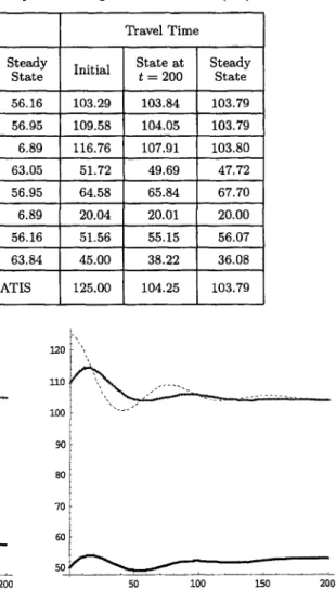
Travel T i m e
Initial State at Steady t -- 200 State 103.29 103.84 103.79 109.58 104.05 103.79 116.76 107.91 103.80 51.72 49.69 47.72 64.58 65.84 67.70 20.04 20.01 20.00 51.56 55.15 56.07 45.00 38.22 36.08 125.00 1 0 4 . 2 5 103.79
~.oo~°
) " . ,
80 60 50 i00 150 200Figure 2. Evolutions of p a t h 1 flow dynamics and P ~ (M1). (Dashed line: predicted unit TTLpath 1,,~
OD travel time by ATIS; gray line: travel time of p a t h 1; black line: flow of p a t h 1.)
120 110 i00 90 80 70 60 50_ 50 100 150 200
Figure 3. Evolutions of p a t h 2 flow dynamics and p t (M1). (Dashed line: predicted unit TTLp~th 2,,~
OD travel t i m e by ATIS; gray line: travel time of p a t h 2; black line: flow of p a t h 2.)
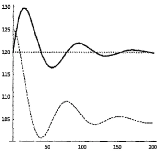
Vehicular Flow Dynamics 120 100 40 I 20 ~%- j l ~ ~ r ~ ~ ~ . . . ~ . . . ___ ~ . . . 50 100 150 200 125 120 ns ~ no ! / "\ i ; , los ,,, / , . . . . 50 I00 150 200
Figure 4. Evolutions of path 3 flow dynamics and t (M1). (Dashed line: predicted unit PTTLpath 3,,,
OD travel time by ATIS; gray line: travel time of path 3; black line: flow of path 3.)
Figure 5. Evolutions of predicted OD travel time by ATIS and ETD~ (M1). (Dashed line: predicted OD travel time by ATIS; dotted line: OD demand; gray line: sum of path flows.)
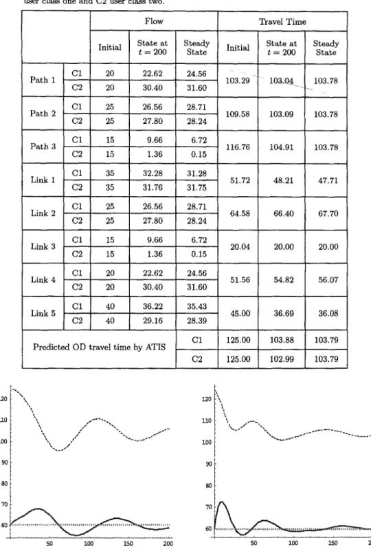
Table 3. Results of numerical example for M2. Two-class users model with identical predicted OD travel time for two user classes, i.e., (15) with n ---- 2; C1 denotes user class one and C2 user class two.
Flow Travel Time
Initial State at Steady State at Steady t -- 200 State Initial t ---- 200 State
C1 20 21.95 22.23 Path 1 103.29 1 0 3 . 7 9 103.79 C2 20 31.84 33.94 C1 25 25.81 26.08 Path 2 109.58 103.80 103.79 C2 25 29.30 30.88 C1 15 9.55 6.62 Path 3 116.76 105.72 103.79 C2 15 1.57 0.25 C1 35 31.50 28.85 Link 1 51.72 48.67 47.71 C2 35 33.41 34.19 C1 25 25.81 26.08 Link 2 64.58 66.76 67.71 C2 25 29.30 30.88 C1 15 9.55 6.62 Link 3 20.04 20.00 20.00 C2 15 1.57 0.25 C1 20 21.95 22.23 Link 4 51.56 55.11 56.08 C2 20 31.84 33.94 C1 40 35.36 32.70 Link 5 45.00 37.05 36.08 C2 40 30.87 31.13
Predicted OD travel time by ATIS 125.00 1 0 3 . 8 8 103.79
517
is c o n n e c t e d b y t h r e e p a t h s d e n o t e d as p a t h 1 = {link 1, link 4}, p a t h 2 = {link 2, link 5}, a n d p a t h 3 -- {link 1, link 3, link 5}, respectively. T h e p a r a m e t e r s of t h e link cost f u n c t i o n s are set in Table 1 w i t h t h e s a m e f u n c t i o n f o r m as ca(f~) = Aa + B,~(fUka) 4.
T h e following t h r e e examples (M1, M2, a n d M3) were solved using t h e h i g h - o r d e r R u n g e - K u t t a n u m e r i c a l m e t h o d w i t h t h e O D d e m a n d fixed as 120. T h e initial conditions, a s s u m e d identical p a r a m e t e r s of t h e p r o p e n s i t y of p a t h flow d y n a m i c s , a n d p a r a m e t e r s t o d e n o t e t h e sensitivity of p r e d i c t e d travel t i m e d y n a m i c s for t h e h o m o g e n e o u s user m o d e l (M1), i.e., (9), are given as (h 0, h2, h 3 , 0 0 c 0, c~,~) -- (40, 50, 3 0 , 1 2 5 , - 0 . 0 0 0 6 , 0.1). Table 2 shows t h e d y n a m i c s of flows, travel times, a n d p r e d i c t e d O D travel times b y A T I S at three different s t a t e s for t h e first example.
125 120 115 110 ~Y 105 ! 12,5 120 1175 100 50 100 150 200 2 2 . 5 20 i~ 17.5 1 2 . 5
!
lo i
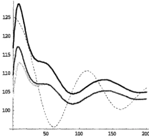
50 i00 150 200Figure 6. Travel time evolutions of M2. (Dashed line: predicted OD travel time; light gray line: path 1; medium gray line: path 2; black line: path 3.)
Figure 7. Path flow evolutions of user class one in M2. (Light gray line: path 1; medium gray line: path 2; black line: path 3,)
2o
i
I - 50 100 150 200 120 115 1/0!
\
105 ; ',./'. /'-'~.. , " . . . - - " " . . . : ' - ' : . . . - 50 I00 150 200Figure 8. Path flow evolutions of user class two in M2. (Dashed line: predicted OD travel time; light gray line: path 1; medium gray line: path 2; black line: path 3.)
Figure 9. Evolutions of predicted OD travel time by ATIS and E T D ~ (M2). (Dashed line: predicted OD travel time by ATIS; dotted line: OD demand; gray line: sum of path flows.)
518 H.-J. CHO AND M.-C. HWANG
50 100 150 200 125 120 115 110 105 --I 50 I00 150 200
Figure 10, Evolutions of path travel times and C1 predicted OD travel times for M3. (Dashed line:
C1 predicted OD travel time; light gray line: path
1; medium gray line: path 2; black line: path 3.)
Figure 11. Evolutions of path travel times and C2 predicted OD travel times for M3. (Dashed line: C2 predicted OD travel time; light gray line: path 1; medium gray line: path 2; black line: path 3.)
Vehicular Flow Dynamics
Table 4. Results of numerical example for M3. Two-class users model with user- specific predicted OD travel time for two user classes, i.e., (16) with n----2; C1 denotes user class one and C2 user class two.
Flow Travel Time
Initial State at Steady Initial State at Steady t --- 200 State ~ = 200 State C1 20 22.62 24.56 -t P a t h 1 103.29 103.04 103.78 C2 20 30.40 31.60 . . . . -- C1 25 26.56 28.71 P a t h 2 109.58 103.09 103.78 C2 25 27.80 28.24 C1 15 9.66 6.72 P a t h 3 116.76 104.91 103.78 C2 15 1.36 0.15 C1 35 32.28 31.28 Link 1 51.72 48.21 47.71 C2 35 31.76 31.75 C1 25 26.56 28.71 Link 2 64.58 66.40 67.70 C2 25 27.80 28.24 C1 15 9.66 6.72 Link 3 20.04 20.00 20.00 C2 15 1.36 0.15 C1 20 22.62 24.56 Link 4 51.56 54.82 56.07 C2 20 30.40 31.60 C1 40 36.22 35.43 Link 5 45.00 36.69 36.08 C2 40 29.16 28.39 C1 125.00 103.88 103,79 Predicted OD travel time by ATIS
C2 125.00 102.99 103.79 519 120 110 i00 90 80 70 60 "\
\
\ ,/i 50 i00 150 200Figure 12. Evolutions of C1 predicted OD travel time by ATIS and ETD~w (M3). (Dashed line: C1 predicted OD travel time by ATIS; d o t t e d line: OD demand; gray line: sum of p a t h flows for C1.)
120 110 i00 90 80 70 6 0 \ 50 i00 150 200
Figure 13. Evolutions of C2 predicted OD travel time by ATIS and ETD~w (M3). (Dashed line: C2 predicted OD travel t i m e by ATIS; d o t t e d line: OD demand; gray line: sum of p a t h flows for C2.)
It is clear that the steady state satisfies the Wardrop's user equilibrium and the predicted OD travel time is equal to the path travel times of which path flows are positive simultaneously. Numerical results by the evolutions of network dynamics illustrated from Figures 2-5 also show that the path flow increases (decreases) as path travel time is less (more) than the predicted OD
520 H.-J. C H O A N D M . - C . H W A N G 2 0 / ' " \ , J +''= *"~+%, <, J % I :> 1 0 l | 2 0 t" 1 0 i ~ ~ Q 200 ~ 100 ~ 0 2 ~
Figure 14. Path flow evolutions of C1 in M3. (Light gray line: path 1; medium gray line: path 2; black line: path 3.)
Figure 15. Path flow evolutions of C2 in M3. (Light gray line: path 1; medium gray line: path 2; black line: path 3.)
travel time and predicted OD travel time increases (decreases) as OD demand is more (less) than the sum of p a t h flows.
The second example is set for the multiclass user model with identical predicted OD travel time by ATIS (M2), i.e., (15) as n = 2. Parameters of the propensity of p a t h flow dynamics for the two classes are assumed to be different but the same within a user class. T h e y are -0.0006 and - 0 . 0 0 3 for class one and class two, respectively. T h e other inputs of the second example are the same as the previous case, and the outputs reveal t h a t the steady state is qualified as a Wardrop's user equilibrium. The embedded mechanisms of adjustments are also sustained by the results in Table 3 and Figures 6-9. However, two additional facts are found t h a t sensible users occupy b e t t e r routes sooner t h a n less sensible users in the evolution process until equilibrium is reached, and the ratio of first-class users to second-class users for three paths at a steady state is different from t h a t at the initial status. T h e latter one can be interpreted as the result of the former and evidently due to various parameters of the propensity of path flow dynamics. Moreover, we remind readers t h a t the shares of OD demand for two user classes might be changed in the processes.
Finally, the third case is prepared for the two-class user model with the user-specific predicted OD travel time by ATIS (M3), i.e., (16) as n = 2. All inputs are the same as the second example but each user class is provided with a dedicated OD travel time predicted by ATIS and an equal OD demand, i.e., D l l = D21 = 60. Unsurprisingly, the outcome, shown in Table 4 and Figures 10-15, follows the asymptotic behaviors claimed in the previous section. It is also observed t h a t the adjustment speeds in M3 are less t h a n t h a t in M2 from the initial conditions to the 200 th time state. It is in t h a t the path flow dynamics are limited by a fixed and smaller OD demand for user class two in M3. However, it seems to be reasonable t h a t the OD demand ratio of user class one to user class two should not be overly distorted in the evolution processes even though the total OD demand is kept unchanged. This point should be a necessary check when M2 is implemented into the empirical study.
6. C O N C L U S I O N S
In this paper, the authors deal with further developments of vehicular network dynamics in a day-to-day time scale by using a nonlinear dynamical system approach. Incorporating the total perceived travel time loss (or saving) into the proposed models, time change rates of path flows are generated on a flow-weighted base to prevent the p a t h flow dynamics from being insensible of flow level which have been formulated in previous studies [4,24]. Issues of heterogeneous users and corresponding means of providing travel information are also considered in multiclass users models
Vehicular Flow Dynamics 521
by dividing path users into several classes according to the sensitivity of path flow dynamics due to the total perceived travel time loss (or saving) for each user class. The equilibrium solutions of presented models are analyzed mathematically to be the Wardropian equilibria and proved to be asymptotically stable in the sense of Lyapunov. The lemma of the Lipschitz condition for the proposed dynamical system is a key in the proof of existence and uniqueness by the way of the fundamental theorem of differential equations. Based on these results, the proposed models build an analytical linkage between the Wardrop's user equilibrium and the empirical adaptability of route preference under the operations of intelligent transportation systems.
R E F E R E N C E S
1. J.L. Horowitz, The stability of stochastic equilibrium in a two link transportation network, Transportation Research 18B, 13-28, (1984).
2. M.J. Smith, The stability of a dynamic model of traffic assignment--An application of a method of Lyapunov,
Transportation Science 18, 245-252, (1984).
3. E. Cascetta and G.E. Cantarella, A day-to-day and within day dynamic stochastic assignment model, Traspn. Res. 25A, 277-291, (1991).
4. T.L. Friesz, D. Bernstein, N.J. Mehta, R.L. Tobin and S. Ganjalizadeh, Day-to-day dynamic network dise- quilibria and idealized traveler information systems, Operations Research 42, 1120-1136, (1994).
5. G.E. Cantarella and E. Cascetta, Dynamic processes and equilibrium in transportation networks: Towards a unifying theory, Transportation Science 29, 305-329, (1995).
6. D. Watling, Stability of the stochastic equilibrium assignment problem: A dynamical systems approach,
Transportation Research 33B~ 281-312, (1999).
7. G.L. Chang and H.S. Mahmassani, Travel time prediction and departure time adjustment behavior dynamics in a congested traffic system, Transportation Research 22B, 217-232, (1988).
8. H.S. Mahmassani, Dynamic models of commuter behavior: Experimental investigation and application to the analysis of planned traffic disruptions, Transportation Research 24A, 465-484, (1990).
9. T.Y. Hu and H.S. Mahmassani, Evolution of network flows under real-time information: A day-to-day dy- namic simulation-assignment framework, Transportation Research Record 1493, 46-56, (1995).
10. T.Y. Hu and H.S. Mahmassani, Evolution of network flows under real-time information and responsive signal control systems, Transportation Research 5C, 51-69, (1997).
11. M. Ben-Akiva, A. dePalma and I. Kaysi, Dynamic network models and driver information systems, Trans- portation Research 25A, 251-266, (1991).
12. Q. Yang and H.N. Koutsopoulos, A microscopic traffic simulator for evaluation of dynamic traffic management systems, Transportation Research 4C, 113-129, (1996).
13. A.K. Ziliaskopoulos and L. Rao, A simultaneous route and departure time choice equilibrium model on dynamic networks, International Transactions in Operational Research 6, 21-37, (1999).
14. V. Astarita, V. Adamo, G.E. Cantarella and E. Cascetta, A doubly dynamic traffic assignment model for planning applications, In Proc. of 1~ th International Symposium on Transportation and Traj~ie Theory,
(Edited by A. Ceder), pp. 373-386, Pergamon Press, London, U.K., (1999).
15. D. Watling, A stochastic process model of day-to-day traffic assignment and information, In Behavioural and Network Impacts of Driver Information Systems, (Edited by R. Emmerink and P. Nijkamp), pp. 115-139, Ashgate Publishing Ltd., (1999).
16. D.K. Merchant and G.L. Nemhauser, A model and an algorithm for the dynamic traffic assignment problems,
Transportation Science 12, 183-199, (1978).
17. B.N. Janson, Dynamic traffic assignment for urban road networks, Transportation Research 25B, 143-161, (1991).
18. T.L. Friesz, D. Bernstein, T.E. Smith, R.L. Tobin and B.W. Wie, A variational inequality formulation of the dynamic network user equilibrium problem, Operations Research 41, 179-191, (1993).
19. B. Ran, D. Boyce and L. Le Blanc, Toward a new class of instantaneous dynamic user-optimal traffic assign- ment models, Operations Research 41, 192-202, (1993).
20. H.K. Chen and C.F. Hsueh, A model and an algorithm for the dynamic user-optimal route choice problem,
Transportation Research 32B, 219-234, (1998).
21. H.K. Lo and W.Y. Szeto, A cell-based dynamic traffic assignment model: Formulation and properties, Mathl. Comput. Modelling 35 (7/8), 849-865, (2002).
22. J.G. Wardrop, Some theoretical aspects of road traffic research, Proceedings of the Institute of Civil Engineers Part II~ 325-378, (1952).
23. T.L. Friesz, Transportation network equilibrium, design and aggregation, Transportation Research 19A, 413-427, (1985).
24. T.L. Friesz, D. Bernstein and R. Stough, Dynamic systems, variational inequalities and control theoretic models for predicting time-varying urban network flows, Transportation Science 30, 14-31, (1996).
25. M. Carey, Stability of competitive regional trade with monotone demand/supply functions, Journal of Re- gional Science 20, 489-501~ (1980).
522 H.-J. CHO AND M.-C. HWANG
26. L. Perko, Differential Equations and Dynamical Systems, Springer-Verlag, (1996).
27. K.T. Alligood, T.D. Sauser and J.A. Yorke, Chaos: An Introduction to Dynamical Systems, Springer-Verlag, New York, (1997).