國立交通大學
工業工程與管理學系
博士論文
需求不確定下控檔片之管理
Managing Control and Dummy Wafers
under Demand Uncertainty
研 究 生:楊懿淑
指導教授 :張永佳 博士
需求不確定下控檔片之管理
Managing Control and Dummy Wafers
under Demand Uncertainty
研究生 : 楊 懿 淑 指導教授: 張 永 佳 博士 Student: Yi-Shu Yang Advisor:Dr. Yung Chia Chang
國立交通大學
工業工程與管理學系
博士論文
A Dissertation
Submitted to Department of Industrial Engineering and Management College of Management
National Chiao Tung University in partial Fulfillment of the Requirements
for the degree of Doctor of Philosophy
in
Industrial Engineering and Management
July 2009
Hsinchu, Taiwan, Republic of China
i
需求不確定下控檔片之管理
學 生:楊 懿 淑 指導教授:張永佳 博士
國立交通大學工業工程與管理學系
摘要
半導體製作過程中控檔片(Control and Dummy Wafers) 的主要功能在於確保 晶圓產品的品質與製程穩定。大量的控檔片並非產品卻不可或缺,一但短缺則會 導致製程停頓與交期延誤,間接會提高成本和降低獲利。故有效的管理控檔片是 晶圓製造過程中重要的議題。 本研究主要探討控檔片之降級法則與需求服務水準兩種問題,目的是在多期 多產品不確定需求前提下最小化總成本。本研究以兩階段隨機規劃模型求出新片 的供給數量、降級的數量、方式與途徑,探討降級法則;再以機遇限制規劃模型 滿足預設的需求服務水準,並提出利用滾動時窗法將機遇限制規劃模型轉換成等 價的動態線性規劃模型求解。經由實例驗證,本研究所設計之控檔片管理模式在 實務上因將需求不確性列入考慮,故提高其應用上之有效性。 關鍵詞:控檔片、隨機規劃、機遇限制規劃、需求不確定性。
ii
Managing Control and Dummy Wafers
under Demand Uncertainty
Student : Yi Shu Yang Advisor: Dr. Yung Chia Chang
Department of Industrial Engineering and Management National Chiao Tung University
ABSTRACT
The first subject of this dissertation is to study a realistic planning environment in wafer fabrication for the control and dummy wafers problem (C/DWP) with uncertain demand. A two-stage stochastic programming model is developed based on scenarios and solved by a deterministic equivalent large linear programming model. The model explicitly considers the objective to minimize the total cost of C/D wafers. A real-world example is given to illustrate the practicality of a stochastic approach. The results are better in comparison with deterministic linear programming by using expectation instead of stochastic demands. The model improved the performance of C/D wafers management and the flexibility of determining the downgrading policy. For the inventory management with service level, a chanced-constrained model is developed to minimize the total cost and to keep satisfaction of customer with pre-specified probability level. Based on rolling horizon method, this model is transformed into a dynamically equivalent linear problem. A numerical example problem is illustrated to provide information for setting customer satisfaction levels and unfolding effective inventory management options.
Keywords: control and dummy wafers, stochastic programming, chance-constrained programming, demand uncertainty
iii
致謝
在此向指導教授張永佳老師致上最深之感謝與最高之敬意,您細心的指導使 得本論文得以完成;同時,感謝唐麗英教授、陳澤雄教授、余豐榮教授、王春和 教授與鄧世剛 此外,感謝先生與兒子十年來的支持與疼惜,讓我能無後顧之憂地完成這一 件事。亦謝謝弟妹與其家人,一直以來互相關心與扶持。當然更要感恩上蒼賜於 我們最棒的父母,讓我們在愛的環境下成長,並學會父親勤儉、自立與利他的人 生觀和母親獨立、樂觀、重情義的生活態度。 教授提供寶貴建議,讓此論文更臻完美。 最後,在交大歲月和同學賴春美一起經歷酸甜苦辣,這些都是生命中精采的 樂章,謝謝有你作伴。 楊懿淑 謹誌於國立交通大學工業工程與管理系 97 年 7 月iv
Table of Contents
摘要 ... i ABSTRACT ... ii 致謝 ... iii Table of Contents ... iv List of Figures ... viList of Tables ... vii
Notation ... viii 1. Introduction ... 1 1.1 Motivation ... 1 1.2 Objectives ... 3 1.3 Thesis Outline ... 4 2. Literature Review ... 6 2.1 Downgrading Resource ... 7 2.2 Inventory Management ... 8 2.3 Stochastic Programming ... 11
2.3.1 Two-stage stochastic programming ... 11
2.3.2 Chance-Constrained Programming ... 14
2.4 Normal Transformation ... 17
3. Background Information and Problem Description ... 23
3.1 The PUR Process of C/D Wafers ... 23
3.1.1 Pre-disposition ... 23
3.1.2 In-use ... 24
v
3.2 The Resource Downgrading Characteristic of C/D Wafers ... 26
3.3 Demand Uncertainty ... 27
3.4 Problem Description ... 28
3.4.1 Overview of stochastic management system of C/D wafers ... 28
3.4.2 Assumptions ... 30
3.4.3 Stochastic C/D Wafers Downgrading Problem ... 31
3.4.4 C/D Wafers Service Level Problem ... 32
4. Optimization of Stochastic C/D Wafers Downgrading Problem ... 33
4.1 Formulation of Stochastic C/D Wafers Downgrading Problem ... 33
4.2 Optimization Methodology ... 36
4.2.1 Demand Model and Scenario Construction ... 36
4.2.2 Solution Procedure ... 39
4.3 Implementation of Stochastic C/D Wafers Downgrading Problem ... 39
4.3.1 Numerical Example and Input Information ... 40
4.3.2 Experimental Results and Sensitivity Analysis ... 41
5. Optimization of the C/D Wafers Service Level Problem ... 46
5.1 Formulation of Stochastic C/D Wafers Service Level Problem ... 46
5.2 Optimization Methodology ... 48
5.3 Implementation of chance-constrained C/D Wafers Problem ... 51
5.3.1 Numerical Example and Input Information ... 51
5.3.2 Experiment Results and Sensitivity Analysis ... 52
6. Conclusion Remarks ... 58
6.1 Concluding Remarks ... 58
6.2 Future Research ... 60
vi
List of Figures
Figure 1-1 Applications of C/D wafers in process ... 2
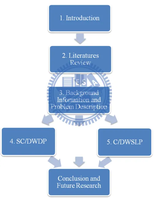
Figure 1-2 Organization of this study ... 5
Figure 3-1 The cyclic relation among PUR process of a C/D wafer. ... 25
Figure 3-2 Multi-level downgrading diagram for C/D wafer ... 25
Figure 3-3 Schematic stochastic C/D wafers management system diagram ... 29
Figure 4-1 Event tree and scenarios for SC/DWD problem model ... 38
Figure 4-2 Sensitivity of values of optimal alternatives ... 45
Figure 5-1 Cost analysis for the base case ... 54
Figure 5-2 Variation of total cost with service level ... 55
vii
List of Tables
Table 4-1 The parameters of demands for each product ... 40
Table 4-2 The number of times for C/D wafer consumed by each product at each grade .... 41
Table 4-3 The unit cost for (holding, recycling/natural downgrading, demand downgrading) ... 41
Table 4-4 Economic benefit analysis for SC/DWDP ... 41
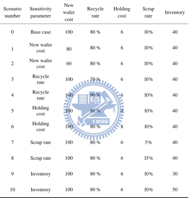
Table 4-5 Parameter values for sensitivity analysis ... 44
Table 5-1 The demands of all products in the last five years ... 51
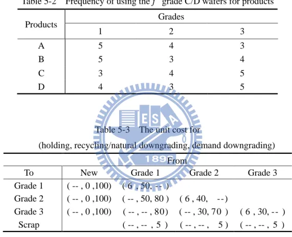
Table 5-2 Frequency of using the jth grade C/D wafers for products ... 52
Table 5-3 The unit cost for (holding, recycling/natural downgrading, demand downgrading) ... 52
viii
Notation
Index Definition Sets
m Product M = {1, 2, …, M}
j Sequencing grade of C/D wafer J = {1, 2, …, J}
k Number of grades changed K = {1, 2, …, J-1}
s Demand scenario ξ = {1, 2, …, S}
t Time period T = {0, 1, …, T}
Notations for stochastic C/D downgrading problem and C/D service level problem
[ ]t j
I Quantity of inventory for the jth [ ]t
j
x0
grade of C/D wafers in period t
Quantity of new C/D wafers released to the jth [ ]t jj x grade in period t Quantity of the jth [ ]t k) j(j x +
grade C/D wafers for recycling in period t
Quantity of the jth grade C/D wafers downgraded to the (j+k)th
[ ]
t js x grade due to demand in period t Quantity of the jth [ ]t m Dgrade C/D wafers scraped in period t
Matrix of demand of the product m in period t
[ ]t j
d Matrix of the integrated demand for the jth m
j
f
grade C/D wafers in period t.
Frequency of using the jth
0
c
grade C/D wafers in the process for product m
ix
jj
c Cost of recycling a C/D wafer at the jth
(n) ij
c
grade/ per unit
Cost of natural downgrading a C/D wafer from the ith grade to the jth
(d) ij
c
grade/ per unit
Cost of demand downgrading a C/D wafer from the ith grade to the jth
(s)
c
grade/ per unit
Cost of scraping a C/D wafer
j
h Cost of holding the jth r
grade C/D wafer
times of recycling for a C/D wafer at the j
j th
u
grade
Minimum level of inventory of the C/D wafers at each grade
Rr Maximum rate of recycled C/D wafers at each grade
Rs Minimum rate of scraped C/D wafers at each grade 1- α Service level
m
µ Expected demand of product m 2
m
σ
Demand variance of product m
( ) [ ]t
s j
d
Total demand for the jth ( )
[ ]
t s jI
grade C/D wafers in period t, (scenario s)
Quantity of inventory for the jth ( )
[ ]t s j
x 0
grade C/D wafers in period t (scenario s)
Quantity of new C/D wafers released to the jth ( )
[ ]t s jj
x
grade in period t (scenario s)
Quantity of the jth ( )( )
[ ]
t s k j j x +grade of the C/D wafers for recycling or external downgrading in period t (scenario s)
Quantity of the jth grade of the C/D wafers downgraded to the (j+k)th grade due to demand in period t (scenario s)
1
1. Introduction
1.1 Motivation
Control and dummy (C/D) wafers are indispensable to manufacturing processes in
semiconductor wafer fabrication. Control wafers are used to measure the refraction indices
and etching rates in order to test the quality of equipment and monitor the process prior to
risking the real product wafer. This ensures process stability and normal equipment operation.
Control wafers may also be used with products together as proof of product quality in the
process by measuring particle numbers and film thickness. Dummy wafers are used to
distribute heat uniformly inside the furnaces. Each inspection item requires C/D wafers for
different devices. Figure 1-1 represents an overview of the applications of C/D wafers in a
wafer fabrication. Any lack or surplus of C/D wafers may cause the loss of equipment
capacity and production movement because they occupy equipment capacity of wafer
fabrication, not only affecting production planning but also decreasing process yield.
Besides the cost and quality issues, the lifecycles of C/D wafer make management a real
challenge. The major characteristics of C/D wafers is that they can repeat the same functional
test several times until they fail to conform to quality specifications related to requirements
2
process is pulled from the inventory. If the number of C/D wafers is not enough, new C/D
wafers are released. Once the C/D wafer is used, it has to be checked whether it can be reused
or not. If yes, it can either return back to the inventory, or to a lower grade based on the
demand. Good management can reduce the number of C/D wafers brought in to the
manufacturing process and improve the efficiency of C/D wafer usage.
Therefore, the main challenges of C/D wafer management are downgrading problem
and inventory control.
Figure 1-1 Applications of C/D wafers in process
3
1.2 Objectives
C/D wafer management is a crucial issue of complexity in the wafer fabrication, because
it needs to consider not only downgrading policy, release rule, and inventory control, but also
service level under demand uncertainty. Even though many researchers have focused on C/D
wafers management, little study has been done under demand uncertainty which is a
realization of nature. In real world, the manufacturer has to meet the demand for different
products according to the service level requirements set by its customers. To capture the
trade-off between customers satisfaction and production costs, it makes C/D wafers
management effectively and efficiently. This research attempts to:
1. Develop a two-stage stochastic programming model to minimize the total cost of
C/D wafers and to set the quantities of new C/D wafers released and C/D wafers
recycled or downgraded to meet the stochastic demands of each grade.
2. Develop a chance-constrained programming model to minimize the total cost of
C/D wafers and to make production and C/D wafers sourcing decisions during the
planning horizon subject to the service level requirements set by customers.
To attain the mission of the stochastic C/D wafers downgrading problem (SC/DWDP), a
4
linear model and easier solutions by utilizing a single large equivalent LP model. Next, to
achieve the objectives of C/D wafers service level problem (C/DWSLP) constructed by a
chance-constrained programming model, an approach is proposed to decide an appropriate
C/D wafer quantity for each grade in each period. The approach includes three phases: (i)
transforming the empirical cumulative demand data, if it is non-normal, into a set of data
which is approximately normal distributed, (ii) transforming the chance-constrained
programming model into an equivalent integer programming, and (iii) using rolling horizon
method to solve the problem dynamically.
1.3 Thesis Outline
The remaining of this study is organized as follows.
Chapter 2 reviews four portions, viz., (i) downgrading resource (ii) inventory
management (iii) stochastic Programming and (iv) normal Transformation. Chapter 3
describes the background information including: the PUR process of C/D wafers, the resource
downgrading characteristics of C/D wafers, demand uncertainty, and assumptions of this
study. In chapter 4, a two-stage stochastic programming model is proposed, while a
5
future research are given in chapter 6. Figure 1-2 illustrates the architecture of these six
chapters in this study.
6
2. Literature Review
The purpose of using C/D wafers is to assure that the wafer manufacturing process
operations meet the required manufacturing specifications. Downgrading resources and
inventory control are two characteristics of C/D wafer management. To properly account for
product demand fluctuate, this research considers that the demand is uncertain.
Rare researches have been conducted on C/D wafer management since Wong and Hood
[76] used discrete event simulation to run a hypothetical fab model with an industry-standard
CMOS base process. They did not provide a method for efficiently managing test wafers but
only examined the impact of test wafers on process cycle time, wafer throughput, and fab line
equipment capacity requirements. Chen et al. [17] pointed out the issues about C/D wafer
management. Later, Chen et al. [19] proposed a pull system to manage C/D wafers in order to
increase the efficiency of C/D wafers. According to the above, downgrading rules and
inventory control are the keys of a good C/D wafers management. Therefore, the literature
review includes downgrading resources, inventory management, stochastic programming, and
normal transformation. The first two topics are related to the C/D wafer management, while
7
2.1 Downgrading Resource
Due to the reuse and downgrading of the C/D wafers, resource downgrading problem is
quite different from other production problems. Some researchers focused on downgrading
rules. Chen, et al. [18] suggested downgrading and release rules for C/D wafers. Foster, et al.
[32] studied test wafer consumption by simulation. Although simulation can realize stochastic
events and observe the effects by the current state of the system during a specific simulation
run, it needs more time to produce results, and the randomness does not guarantee the same
results between different runs. On the other hand, Foster, et al. [32] also suggested “lowest
inventory first” downgrading rule which only can yield suboptimal solution. Chung, et al. [23]
proposed a linear programming model for the C/D wafers downgrading problem to minimize
the total cost of C/D wafers by using expected demand in the photolithography area of a wafer
fab. Wu, et al. [77] aimed to minimize the long-term daily use of brand-new C/D wafers in a
fab by a linear programming model. Özelkan and Çakanyildirim [57] represented a resource
downgrading problem as a network model with side constraints, which results in an integer
programming formulation. Of the above, little work has been done to include the uncertainty
of demands so as to meet the rapidly changing demands of the future. Liou, et al. [53]
established a capacity forecast model for C/D wafers for decision support instead of basing it
8
mentioned that Motorola MOS12 designed a re-use matrix to determine the possible uses for
C/D wafers. However, it is manual and thus has limitations due to the complexity of
identifying downgrading paths and controlling the inventory of C/D wafers.
This downgrading substitution structure also occurs in some other practical settings, for
example, in the steel industry by Wagner et al. [72], memory chips by Leachman [51],
inventory policies of priority by Duran et al. [30], and semiconductor chips by Hsu et al. [41].
2.2 Inventory Management
Inventory has been one of the most investigated areas of research. Early work done by
Harris [38] on inventory management goes back to the classical economic lot size model
which assumes a steady demand and holding costs over time. Deterioration of products is
realistic in many inventory systems. In determining the optimal inventory policy of product,
the loss due to deterioration should be taken into account. Ghare and Schrader [33] initiated
the analysis of deteriorating inventory by establishing a classical no-shortage inventory model
with a constant rate of decay. Covert and Philip [25] extended Ghare and Schrader’s model by
establishing an economic order quantity (EOQ) model for a variable rate of deterioration with
a two-parameter Weibull distribution. Later, Kar et al. [48] proposed a deterministic
9
assumed linearly increasing, time-dependent over a fixed finite time horizon. To fit a more
general inventory feature, Chang and Dye [13] developed an EOQ model to find the optimal
total cost savings for deteriorating items with varying rate of deterioration during the special
replenishment period. Chung and Tsai [22] developed an inventory model for deteriorating
items with the demand of linear trend and shortages during a finite planning horizon. A line
search was applied in a simple solution algorithm to determine the optimal interval without
considering stock-outs. Chang et al. [14] proposed a finite time horizon EOQ model taking
into accounts the followings: a time-varying deterioration rate, time value of money,
shortages and permissible delay in payments.
In practice, demand and service level may influence safety inventory. Inventory models
have been continually modified to accommodate to more practical issues of the production
planning and the real inventory systems. For a large family of lead time demand distributions,
Platt et al. [60] declared that the optimal policy depends on two parameters: the fill rate and
the EOQ scaled by the standard deviation of demand over the constant lead time. Silva Filho
[68] proposed the cumulative demand is a random variable represented by a compound
Poisson process, since the demand affects the inventory system. Gupta et al. [36] utilized a
stochastic framework to provide quantitative guidelines for setting customer satisfaction
10
Maiti [5] assumed that the production rate is a variable. They also presented inventory models
in which the production rate depends on either on-hand inventory or demand. Das et al. [27]
developed a multi-item inventory model with quantity-dependent inventory costs and
demand-dependent unit cost under imprecise objective and restrictions. Both geometric
programming (GP) and gradient-based nonlinear programming (NLP) methods are used to
solve the problem. Rao et al. [65] modeled a single period multi-product inventory problem
with uncertain demand and one-way product substitution in the downward direction. Pal et al.
[58] constructed a deterministic inventory model with a stock-dependent demand rate and a
constant item deteriorating rate. In addition, a fuzzy geometric programming (FGP) method is
used to solve two highly nonlinear equations generated from the model. Duran et al. [30]
provided tools for managing production and inventory tactically when customers differ in
their willingness to pay and to wait. Many other references about multi-echelon inventory
management in supply chains with uncertain demand and lead times appear in Gumus and
Guneri’s survey [34].
For C/D wafers in the semiconductor industry, majority of researches have been focused
on controlling inventory with deterministic demand, inventory management under uncertain
demands has received relatively little attention. Chung, et al. [24] used a non-linear program
11
approximately normal distribution, the optimal solutions were based on deterministic
expected values to simplify stochastic events and dynamics that might reach misleading
solutions.
2.3 Stochastic Programming
A great quantity of research has been conducted on C/D wafer management but most
was based on the assumption of known or expected demand. Chung et al. [23] assumed the
demand of C/D wafers is constant. Later, Chung et al. [24] used a non-linear program to set a
safe inventory level for control wafers but assumed that demand follows an approximately
normal distribution. Their optimal solutions were based on deterministic expected values to
simplify stochastic events and dynamics that might reach misleading solutions.
2.3.1 Two-stage stochastic programming
Uncertainty is one of the main characteristics of semiconductor manufacturing systems.
To handle uncertainty, it is appropriate to use a two-stage stochastic programming (SP) with
recourse, which was first independently presented by Dantzig [26] and Beale [3]. It is a
dynamic linear programming model characterized by uncertain future outcomes for some
12
(
)
[
x ω]
cx E Q , min Z = + ω (1) Subject to 0 ≥ ≥ b x Ax , (2) where Q(
x, ω)
= min f( )
ω ⋅y (3) Subject to( )
ω y d( )
ω B( )
ω x D = + (4) 0 ≥ y ,ω
∈Ω.The model is separated into two stages. At the first stage, referred to Equations (1) and
Equation (2), the decision variables are chosen to minimize the direct cost and expected
recourse cost that faces the recourse action taken. At the second stage, referred to Equations
(3) and Equation (4), the decision variables are chosen due to the future uncertainty defined
by probability space (Ω, P). Matrix A, vector b, and vector c are known with certainty. The function Q(x, ω), is referred as the recourse function. The technology matrix D(ω), the right-hand side d(ω), the inter-stage link matrix, B(ω), and the objective function coefficients f(ω) may be random. For a realization ω, the corresponding recourse action y is determined
by Q(x, ω). Therefore, the optimal solution of the objective function hedges against all possible events ω∈Ω that might occur in the future. Kall [47] suggests that “here and now”
13
(HN) and “wait and see” (WS) are two different solution approaches to the stochastic
programming. The WS approach assumes that the decision maker would not make the optimal
decision until the outcome of a random variable can be observed. It is clear that such a
solution is not implemented. The HN approach represents the true stochastic optimization
solution without knowledge of the realization of random variables. A number of different
algorithmic approaches have been proposed for solving the stochastic linear programming
stated above, Equations (1) – (4). Refer to Wets [74] for an investigation of the recourse
problem. Later, Wets [75] surveyed the use of large-scale linear programming techniques.
Using mathematical programming techniques seemed to be one of the promising approaches
to solve stochastic problem in some special cases, since stochastic models address the
shortcomings of deterministic models directly. There are two measures to evaluate whether
stochastic approach can be nearly optimal or nearly accurate: the expected value of perfect
information (EVPI) and the value of the stochastic solution (VSS). EVPI and VSS give the
motivation for stochastic programming in general and remain a key focus for the sensitivity
analysis. EVPI measures the value of knowing the future with certainty while VSS assesses
the value of knowing and using distributions on future outcomes.
Uncertain demand is a realized nature of production process, so a lot of researches in
14
decisions. Bakir et al. [2] studied a realistic planning environment for a multi-product
multi-period with stochastic demand. The normally distributed stochastic demand is
approximated by a discrete approximation method. Gupta et al. [35] proposed a two-stage
stochastic programming approach for incorporating demand uncertainty in multisite midterm
supply chain planning problem. At the expense of imposing the normality assumption for the
stochastic product demands, Gupta et al. [35] evaluated the expected second stage costs by
analytical integration yielding an equivalent convex mixed-integer nonlinear problem. Zhang
et al. [82] consider a discrete-time capacity expansion problem involving multiple families
and multiple machine types, and non-stationary stochastic demand. They used a novel
assumption that demand can be approximated by a distribution in order to allow them to solve
the problem as a max-flow, min-cut problem.
There has been a large variety of applications for stochastic programming; for example,
fleet assignment by Ferguson and Dantzig [31], capacity planning by Christie and Wu [21],
water resource management by Watkins et al. [73], and production planning by Leung et al.
[52]. Many other references appear in King’s survey [49].
2.3.2 Chance-Constrained Programming
15
[15] were the pioneers who proposed chance constrained programming (CCP) as a means of
managing uncertainty and probability. It provides a powerful means of modeling stochastic
decision system which has ability to meet the constraints with certain reliability in an
uncertain environment. The general formulation of CCP is as Equation (5) – (7):
min Zccp = cx (5) Subject to 0 0 x b A ≥ (6)
[
]
where[ ]
, , i , ,I P Aix≥hi ≥α ,i αi ∈ 0 1 =1 (7)Let ξi =
(
Ai,hi)
, ∀i=1,,I, be a random vector on the probability space (Ω, F, P). If the Ai is a row vector, the ith constraint is called individual constraint. If Ai is a r×c matrixwith r >1, then the ith
I , , i h x a P r j i c k jk j ij 1 1 1 = ∏ ≥ ∑ ≥ = = β
constraint is referred to as joint chance constraint. When the stochastic
variables are independent, then the joint chance-constraint (7) can be decomposed into the
product of the constituting chance-constraints as Equation (8).
(8)
If the stochastic variables are correlated, then the joint probabilities cannot be
16
integration of multivariate probability distributions. Plackett [60] proposed a reduction
formula for multivariate normal integrals.
There are a lot of practical problems which always involve uncertainty and probability.
Chance-constrained programming has been implemented in a variety of fields. For instance,
Petkov et al. [59] proposed a stochastic model to maximize the expected profit subject to the
satisfaction of product demands with pre-specified probability levels, electrical circuit design
by Ji et al. [45], routing problem by Wu et al. [78], soil conservation problem by Zhu et al
[82], path planning for autonomous vehicles by Blackmore et al. [7], reservoir management
by Azaier et al. [1], aggregate production planning by Silva Filho et al. [67], and production
planning and sourcing problem by Yildirim et al. [79]. In general, obtaining the optimal
solution of chance-constrained programming is not tractable. Bitran and Yanasse [6]
considered deterministic approximations to a stochastic production problem on a rolling
horizon basis. They showed that the service level constraint can be transformed into a
deterministic equivalent constraint by specifying certain minimum cumulative production
quantities that depend on the service level requirements. Kumral [50] proposed a combination
of the chance-constrained programming and the genetic algorithm to find the optimal mine
system parameters simultaneously. Jana et al. ([42], [43]) proposed a stochastic simulation
17
the random variables follow some discrete distributions [43] and continuous distributions [42].
Manandhar et al. [55] provided a semantic based on scenarios to model combinatorial
decision problems involving uncertainty and probability, while Prekopa [63] provides a
numerical solution of probabilistic constrained programming models.
2.4 Normal Transformation
For most industrial applications, normality is assumed due to the advantage of the
analytical convenience and existing effective statistical methods. For example, Platt et al. [60]
assumed that the lead time demand is normally distributed, so the asymptotic results can be
used as the EOQ from zero to positive infinity to fit a theoretic curve for the order quantity Q
and the reorder point R. Silva Filho [68] proposed the cumulative demand is a random
variable represented by a compound Poisson process. Because the demand affects the
inventory system, a chanced constraint is used to preserve the inventory constraint explicitly
in a stochastic optimization model. A Gaussian approximation is also proposed to the
compound Poisson process. You et al. [80] used Box-Cox transformation method to transform
the experiment data investigated from microcircuit process. But, for many engineering
operations such as locating pins or automatic sensors, the manufacturing data is often
18
perform process performance analysis. Pezdek [64] demonstrated how the non-normal
characteristic would significantly impact on the data analysis result and the conclusion, thus
convey incorrect process information. If the process characteristic is not normally distributed,
there are two popular approaches to transform the non-normal data into a normal one. First,
Johnson [46] proposed a system of three transformation families for selection of a
transformation to normality. Let X be a random variable and Z be a standard normal variable.
The three transformation families in Johnson system are, respectively as Equation (9) – (11),
(
)
[
(
)
]
{
ε
λ
ε
}
ε
λ
ε
η
γ
+ − − − < < + = ln X X , X Z , (9)(
ε)
ε η γ + − > = ln X , X Z , (10)(
)
[
−]
−∞< <∞ + = − X , X sinh Z γ η 1 ε λ , (11)where - ∞ < γ, ε < ∞, η > 0, and λ > 0 are four parameters. The distribution determined by (9) is called the SB distribution denoted by SB (γ, η, ε, λ). Similarly, the distribution determined by
(10) is called the SL distribution denoted by SL(γ, η, ε), and by (11) called the SU distribution
denoted by SU
[37]
(γ, η, ε, λ). The subscripts, B, L, and U, refer to X being bounded, lognormal, and unbounded, respectively. Hahn and Shapiro gave further description of these
19
families should be used. The next step is to estimate parameters of the transformation family
selected. A moment approach in the selection step is to choose the transformation family
according to which region of the ( β1,β2) plane the estimated third (β1) and fourth (β2
[69]
)
standardized sample moments fall into. Slifker and Shapiro pointed out the major
shortcomings of this procedure such as high mean-square errors and vulnerability to outliers
of the sample third and fourth moments.
Another percentile approach prevails and is in fact mostly adopted in practice. Johnson
[46] proposed a method, which uses four percentiles. Based on symmetrical points, Bukac [12]
suggested procedures for estimating parameters of SB distribution. Later, Mage [54]
presented a method of reducing Bukac’s quadratic equations to a quadratic equation. Slifker
and Shapiro [69] suggested choosing four symmetric standard normal deviates equally spaced
with intervals 2z, i.e. 3z, z, -z, and -3z, admittedly not a serious restriction. Bowman and
Shenton [9] proposed a simple algorithmic solution for normal deviates -sz, -z, z, and sz
where s and z are arbitrary positive constants and s > 1. Meanwhile, Owen [56] proposed the
starship procedure to search out a transformation that most nearly transforms the sample to
normality, which is not only tied to Johnson system but also many possibilities exist for the
transformations. Chou et al. [20] recommended that use the set Z = { z0: z0 = 0.25, 0.26, …,
20
for the Slifker and Shapiro’s estimation formulas. The best-fit Johnson distribution is chosen
to be the one that best transforms the data to normality among the z0 values in Z. However,
this procedure cannot discriminate the SL distribution family from the other two families.
Chen and Kamburowska [16] proposed a procedure, called M procedure, which is consistent
by setting a bound on the parameter to prevent from an incorrect selection when the
underlying distribution is an SL distribution.
Box and Cox [10] modified the family of power transformation proposed by Tukey [71].
Its simple form defined as T λ: y y(λ)
( ) = ≠ = 0 0 1 y, λy ln , λ λ -y y λ λ (12)
The transformation in Equation (12) is defined for y > 0. It is hoped that for some value
of λ, a non-normal data can be fitted to a normal distribution. Box and Cox [10] used the maximum likelihood method to estimate the parameter λ. An analytical expression for the accuracy of maximum likelihood estimate of λ is derived by Draper and Cox [29]. Hinkley [39] used order statistics to estimate the transformation parameter. Later, Hinkley [40]
assumed that there might be a value of λ making the transformed data nearly symmetry and proposed a similar method for choosing a symmetrical transformation based on the
21
d = (sample mean – sample median)/sample scale (13)
If the underlying distribution is symmetric, then the mean and the median must be identical.
Thus, the sample data drawn from such distribution should reflect such property, and a good
estimate of λ should minimize the value of d.
Base on the Tukey’s [71] recommendation with setting λ to –2 ≤ λ ≤ 2, Hinkley [40] proposed a step-by-step procedure for computing the power of Box-Cox transformation
based on moment of percentile may be presented as follows:
Step 1: Choose -2 as an initial guess λ0
Step 2: Transform the original sample by taking the power λ
of λ for a given random sample.
0
Step 3: Calculate d defined in Equation (13) using the inter-quartile range as the sample
scale.
and then find the sample
mean, sample median, and sample inter-quartile range for the transformed
random sample.
Step 4: Check whether d is less than a predetermined precision level. If not, iterate Steps
1-3 by increasing the magnitude of λ by unit of 0.05 as new λc, till the difference
22
Step 5: Use the λ derived from Step 4 as the optimal estimateλˆ. Employ Shapiro-Wilk [66] test to check the normality of the transformed sample.
23
3. Background Information and Problem Description
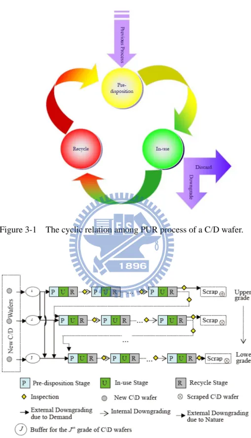
3.1 The PUR Process of C/D Wafers
Cost is only a part of the C/D wafer issue because they also occupy the capacity of
equipment, which is capital intensive. The usage of C/D wafers in wafer manufacturing
processes can be divided into five primary categories, viz., (i) product monitoring, (ii)
equipment monitoring, (iii) preventive maintenance, (iv) the experiment with engineering lots,
and (v) repaired equipment if breakdown. Therefore, good management ought to reduce the
number of C/D wafers brought in to the manufacturing process and improve the efficiency of
C/D wafer usage since the major characteristic of C/D wafers is that they can repeat the same
functional test several times until they fail to conform to quality specifications related to
requirements for cleanliness or thickness. The reuse statuses consist of three processes, viz., (i)
pre-disposition, (ii) in-use, and (iii) recycle stages, termed the PUR process. Figure 3-1
represents the cyclic relation among PUR process of a C/D wafer used in a specific process.
3.1.1 Pre-disposition
Before control wafers are used to monitor production, they have to finish a series of
operations, called pre-dispostion stage, to meet the required specifications. The purpose of
24
3.1.2 In-use
Control wafers are used to monitor process, qualify tools, and develop new process
techniques. To test the wellness of the tool prior to manufacturing the production wafer,
control wafers may be run concurrently with them to perform as a witness to the process, or
may also be used to pilot a process before wafers are committed to a tool. Therefore, output
parameters are taken from the control wafers and adjustments are made to the tool or process
correspondingly. On the other hand, dummy wafers are used on two sides of wafer cassette to
protect the wafers heated uniformly inside the furnaces.
In engineering lots, control wafers are built the designed structure, similar to built onto
the real wafers, to simulate the actual production. The effects of a specific process to the
structure can be studied, characterized, and optimized.
3.1.3 Recycle
After in-use stage, there are some remnants and particles left on the surfaces of C/D
wafers. To reduce the WIP level of C/D wafer, recycle is a key process which polishes off the
contaminants on the top of C/D wafers. This provides a clean C/D wafers re-used back to
25
Figure 3-1 The cyclic relation among PUR process of a C/D wafer.
26
3.2 The Resource Downgrading Characteristic of C/D Wafers
The major characteristic of C/D wafers is that they can repeat the same functional test
several times until they fail to conform to quality specifications related to requirements for
cleanliness or thickness. The reuse statuses consist of the pre-disposition, in-use, and recycle
stages, termed the PUR process, illustrated in Figure 3-2 with dotted arrows. We called it
internal downgrading or recycling. Once a C/D wafer no longer conforms to the pre-defined
specifications, it will be scraped or downgraded to lower grade of which the quality
specifications are not so high. Hence, such a kind of downgrading is referred to here as
external downgrading due to wafer quality, indicated by a dotted line and bold arrows in
Figure 3-2. Furthermore, releasing new raw wafers as any grade of C/D wafers or
downgrading C/D wafers that directly bypass the PUR process to lower grades where there is
a deficit of C/D wafers is regarded as external downgrading due to demand, indicated by a
solid line and bold arrows.
Re-use is crucial to cost saving, but without some policy to prioritize and monitor it, the
efficiency of C/D wafer could be decreasing. As a result, more expensive new C/D wafers will
be brought into the manufacturing process. It is easy to see that C/D wafers are used in very
27
management of C/D wafer must focus on identifying appropriate downgrading rules in order
to increase both the recycled usage of C/D wafers and the throughput rates of wafers.
3.3 Demand Uncertainty
The semiconductor industry has become one of the leading industries in the world on
account of rapid shrinkage of product design cycles and life cycles in the consumer
electronics business. Therefore, competition is fierce and the pace of product innovation and
changes in technologies is high. Due to the intensive capital investment, making efficient
usage of current tools and well planning the production are of great important. Consequently,
the demand for semiconductor products is becoming increasingly hard to predict. In the
prevailing intangible business environment, with ever changing market conditions and
customer expectations, it is necessary to consider the impact of uncertainties involved in the
semiconductor industry.
In the past of researches, deterministic models are assumed widely. But this assumption is
rarely true. It is more reasonable to study this kind of “demand-driven” problems under
uncertain environment because deterministic approach may thus yield unrealistic results by
failing to capture the effect of demand variability on the tradeoff lost sales and inventory
28
could lead to either unsatisfied both customers and loss of market share or excessively high
inventory holding costs. Buffa and Taubert [11] state that the normal, Poisson and negative
exponential distributions have been found to be of considerable value in representing demand
functions for inventory management. A classification of different areas of uncertainty is
suggested by Subrahmanyam et al. [70] including uncertainty in prices, demand, equipment
reliability, and manufacturing uncertainty.
3.4 Problem Description
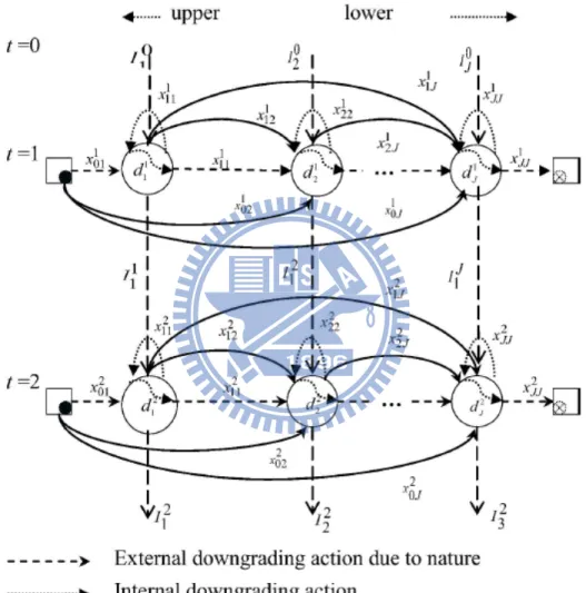
3.4.1 Overview of stochastic management system of C/D wafers
The stochastic management system of C/D wafers is depicted on a simplified
representation of network system, as shown in Figure 3-3. While t = 1 represents the time
period called "here and now", t = 2 is the next time period to "wait and see", and t = 0 is the
previous time period. In Figure 3-3, each node represents the random demand for each grade
of C/D wafers in each period. The solid arrows refer to external downgrading action due to
demand while the segmented arrows refer to external downgrading action due to nature. The
recycle or inventory is presented by dotted arrows. Therefore, in a stabilized system, the
arrivals of C/D wafers at each node are equal to the departures. The inventory at the end of
29
provides the linkage between the periods of the model. To avoid affecting the processes,
backlogging is not allowed.
30
3.4.2 Assumptions
A two-stage stochastic programming model for stochastic control and dummy wafer
downgrading problem (SC/DWDP) and a chanced-constrained programming model for
control and dummy wafer service level problem (C/DWSLP) were constructed for a
theoretical manufacturing system based on the following assumptions:
1. The product mix is given in period t = 1, which represents “now”.
2. The multi-level downgrading rule is applied.
3. Engineering lots are not considered.
4. A shortage of C/D wafers is not allowed.
5. The C/D wafers are classified into J grades.
6. The downgrading graph for each product must be determined in advanced.
7. A lot is the least unit for release, downgrading, and scrap.
8. Each PUR process consists of three processes of operation.
9. The maximum recycle ratio of C/D wafers for each grade is determined to allow the
occurrence of unexpected breakages. (number of recycled to available C/D wafers
31
10. The minimum scrap ratio of C/D wafers for each grade is determined to avoid waste
due to abundance of inventory (number of scraped to available C/D wafers ratio).
11. The demands of products for all time periods are random and empirical.
12. The integrated demands of C/D wafers of each grade at each period are
independent.
3.4.3 Stochastic C/D Wafers Downgrading Problem
To attain the mission of C/D wafers in a fab, we define the stochastic C/D wafer
downgrading problem (SC/DWDP) to minimize the total cost of C/D wafers while
simultaneously determining their inventory policies, downgrading policies, and release rules
for new wafers. We consider that the uncertainty of demands will result in more realistic
planning decisions to meet rapidly changing future demands. Therefore, the purpose of this
dissertation is to develop a two-stage stochastic programming model for SC/DWDP to
minimize the total cost of C/D wafers and to set the quantity of new C/D wafers released and
C/D wafers recycled or downgraded to meet the stochastic demands of each grade. The
proposed stochastic model, which is balanced and hedges against various scenarios, can
describe the real-world production setting more realistically than the static approach can.
32
retaining a linear model and easier solutions by utilizing a single large equivalent linear
programming model. It is more useful and efficient than a simulation approach.
3.4.4 C/D Wafers Service Level Problem
The influencing uncertainty of demands matters in making production decisions of C/D
wafers. This feature makes C/D wafers production management appropriate for the
application of chance-constraint programming (CCP), a more practical and general approach.
The manufacturer has to meet the demand for multi-products according to the service level
requirements set by its customers. And the demand for each product in each period is random.
The C/D wafer service level problem (C/DWSLP) in a chance-constraint manner is presented.
The chanced constraints will hold at least α of time, where α is referred to as the confidence level provided as an appropriate service level by the customers. The rolling horizon approach
is proposed to dynamically transform the model into an equivalent deterministic problem
based on the real life data at each time period and the optimal solution of the preceding
33
4. Optimization of Stochastic C/D Wafers Downgrading Problem
4.1 Formulation of Stochastic C/D Wafers Downgrading Problem
The integrated demand of the jth grade C/D wafers in each time period at the first stage is calculated by Equation (14). Given a scenario at the second stage, Equation (15) calculates
the integrated demand of the jth
[ ] f D[ ], j , , ,J,t , , ,T. d M m t m jm t j 1 2 1 2 1 = = ∑ × = =
grade C/D wafers in each time period.
(14) [ ] [ ] . T , , , t S , , , s J , , , j D f d M m t ) s ( m jm t ) s ( j 1 2 1 2 1 2 1 = = = ∑ × = = ; ; (15)
The production planner’s objective is to minimize the total cost of the C/D wafers and
to determine the supply quantity of C/D wafers at each grade for each period and inventory
quantity at each grade for the next period. The first-stage formulation is given in Equations
(16) – (21). [ ] [ ] [ ] [ ] J [ ]
[
(
S)
]
j j j J j j J k j(j k) ) d ( ) k j ( j J j jj ) n ( ) j ( j J j jj jj J j j , I , X Q E I h x c x c x c x c Z min ξ ξ + ∑ + ∑ ∑ + ∑ ∑ + + ∑ = = = − = + + − = + = = 1 1 1 1 1 1 1 1 1 1 1 1 1 0 0 (16) Subject to34 [ ] d[ ], j , , ,J x rj jj1 ≥ j1 =1 2 (17) [ ] x[ ] x[ ] I[ ] x[ ] , j , , ,J I j J k j(j k) j j k (j k)j ) j )( j ( j 1 2 0 1 1 1 1 1 1 1 0 + + ∑ = + ∑− = = + = − − − 1 -(18) [ ] [ ] [ ] [ ] J , , , j , R x x I x r j k (j k)j ) j )( j ( j jj 1 2 1 1 1 1 1 1 0 1 ≤ = + + ∑ = − − − -(19) [ ] I[ ] x[ ] R , j , , ,J x s ) j ( J k j(j k) j jJ 1 2 1 1 1 1 1 ≥ = + −∑+ = + (20) J , , , j , u I1j ≥ =1 2 (21)
All variables are non-negative integers.
Equation (16) is the objective function that includes the cost of new C/D wafers,
recycling cost, downgrading cost due to natural, downgrading cost due to demand, holding
cost, and the expected cost of the second stage. The operative constraints, of which the first
stage given a specific scenario, are formulated as follows. Equation (17) presents that the
recycling capacity of the C/D wafers must meet the integrated demand of the jth grade. Equation (18) consists of balance constraints representing that the arrivals are equal to the
departures at each grade. The recycle ratio is not more than a positive percentage given by
Equation (19). The scrap rate is not less than a positive percentage given by Equation (20).
35
The second-stage formulation is given in Equations (22) – (27).
( )
[ ] [ ] ( ) [ ] ( ) [ ] + ∑ [ ] ∑ ∑ + ∑ + ∑ + ∑ = = = − = + + = + + = = J j j j(s) J j j J k j(j k)(s) d k) j(j J j j(j )(s) n ) j(j J j jj jj(s) J j j(s) I h x c x c x c x c s Q min 1 2 1 1 2 1 2 1 1 1 2 1 2 0 0 (22) Subject to [ ] d[ ] , x rj jj2(s)≥ j2(s) ,S , , ,J, s , , j =1 2 = 0 1 (23) [ ] x[ ] x[ ] I[ ] x[ ] , I J j k j(j k)(s) ) s ( j j k (j k)j(s) ) s )( j )( j ( j + + ∑ = + ∑ − = + = − − − 0 1 1 1 1 1 1 1 0 -1 ,S , , ,J, s , , j=1 2 = 0 1 (24) [ ] I[ ] x[ ] x[ ] R , x r j-k (j k)j(s) )(s) )(j (j j(s) jj(s) ≤ + + ∑ = − − − 1 1 2 2 1 1 1 2 ,S , , ,J, s , , j=1 2 = 0 1 (25) [ ] I[ ] x[ ] R , x J (j ) s k j(j k)j(s) ) s ( j ) s ( jJ ≥ + −∑+ = + 1 1 2 2 2 ,S , , ,J, s , , j=1 2 = 0 1 (26) [ ] u, Ij2(s) ≥ ,S , , ,J, s , , j=1 2 = 0 1 (27)All variables are non-negative integers.
In the second-stage formulation, Equation (22) represents the objective function of the
second stage. Given a scenario, Equations (23) – (27) are similar to those at the first stage
36
is available for withdrawal in the next period, and provides the linkage between the two stages
of the C/D wafer downgrading problem. All variables are non-negative integers. Finally, the
first and second stage can be summed up into a single large linear programming model.
Therefore, we determine all x’s and I’s to be optimal over all the scenarios because we solve
the large linear programming model for all decision variables simultaneously.
4.2 Optimization Methodology
4.2.1 Demand Model and Scenario Construction
The demands of products are modeled with a geometric Brownian motion process.
Geometric Brownian motion (GBM) was firstly proposed to describe the variation of the
stock price by Black and Scholes [7]. Benavides et al. [4] applied Geometric Brownian
motion as the demand model for IC manufacturing industry, since the historical data is
consistent with Semiconductor Industry Association data. According to Dixit and Pindyck
[28], if Dm
[ ]
t is the demand of product m in period t for C/D wafer downgrading problem, then the rate of change of this demand is assumed to be governed by Equation (28).[ ] D[ ]dt D[ ]dz, t , , ,T m , , ,M.
dDmt =µm mt +σm mt =1 2 ; =1 2 (28)
In Equation (28) dz=εt dt and ε is assumed as a standard normal random variable with t respect to the time interval t. This model of demand implies that the variability of demand
37
increases linearly with the length of demand forecast horizon, so that over a finite time
interval t, the change between the logarithms of demands in two different periods is
distributed as Equation (29): [ ]
( )
( )
[ ] [ ] [ ] ~ N t, t , D D ln D ln D ln m m m m t m t m − = − 2 2 1 2 σ σ µ 1 m T , , , t , M , , , m=1 2 =1 2 (29)In models of decision making under uncertainty, it is essential to represent uncertainties
in a form suitable for quantitative models. It is the most popular method for stochastic
programming to generate a limited number of discrete scenarios that satisfy specified the
random variables. Jarrow and Rudd [44] proposed binary tree with equal probability method
to generate as small number of scenarios as possible and proved it has reasonably good
approximation.
Hence, this method is used to generate the demand distribution of each product at the
second. Note that Dm
[ ]
1 represents the demand of product m in the period t = 1. There are two possibilities of demands for product m in the period t with probability 0.5 as Equation (30).[ ] [ ] ± − =D exp t t Dmt m m m m2 2 1 2 σ σ µ , m=1,2,,M; t=1,2,,T (30)
38
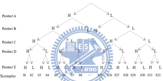
As an approximation example of five products, an event tree with 32 scenarios was
constructed with two branches in each node, which represents high demand or low demand as
shown in Figure 4-1. A scenario is a sequence of events. For example, scenario 1 is the set of
event sequences {H, H, H, H, H} as high demands for each product A to E, respectively.
Figure 4-1 Event tree and scenarios for SC/DWD problem model
No need to reticence, there are no guarantees that those scenarios assembled in this
particular manner can adequately represent the uncertainty of the C/D wafers demands caused
by product mix. To address these potential limitations, sensitivity analyses are presented in a
later section.
S1 S 2 S 3 S 4 S 5 S 6 S 7 S 8 … S 2 5 S 2 6 S 2 7 S 2 8 S 2 9 S 3 0 S 3 1 S 3 2
* H represents high demand and L represents low demand Scenario
39
4.2.2 Solution Procedure
By taking all possible scenarios into account, the first- and second-stage linear
programming models can be summed up into a single large linear programming model. The
objective function of equation (16) can be extended to equation (31) for large-scale linear
programming model. In other words, we are choosing all of x’s and I’s to be optimal over all
the scenarios because we solve for all decisions simultaneously.
[ ] [ ] [ ] [ ] [ ] [ ] [ ] [ ] [ ] [ ] ∑ ∑ ∑ + ∑ ∑ + ∑ ∑ ∑ ∑ + + ∑ + ∑ + ∑ ∑ + ∑ ∑ + + ∑ = = = = = − = + + = = − = = = = = − = + + − = = = S s J j J j j j(s) J j j J k j(j k)(s) ) d ( ) k j ( j ) s ( j S s J j J j jj(s) ) n ( jj J j jj jj(s) J j j(s) ) s ( j J j j j J j j J k j(j k) ) d ( ) k j ( j J j jj ) n ( jj J j jj jj J j j I h x c p x c x c x c p I h x c x c x c x c Z min 1 1 1 2 1 1 2 1 1 1 1 2 1 2 1 2 0 0 1 1 1 1 1 1 1 1 1 1 1 1 0 0 (31)
4.3 Implementation of Stochastic C/D Wafers Downgrading Problem
To investigate the effect of the stochastic management system on the planning,
real-world data is taken from a wafer fabrication factory located in the Science-Based
40
4.3.1 Numerical Example and Input Information
In this production system, regarded as base case, there are five products A, B, C, D,
and E with product mix 5: 7: 3: 4: 1 at the first stage. Based on historical data, we applied a
geometric Brownian motion model and estimated the drift and variance parameters of the
demands for each product, as given in Table 4-1. The monthly throughput target is 640 lots
and the planning period is 28 days. C/D wafers can be categorized into three levels according
to their conditions suitable for use in process. At the end of period t = 0, the inventory
quantity is 30 for grade 1, 40 for grade 2, and 50 for grade 3. The maximum times of
recycling a C/D wafer at each grade is 4, 5, and 6 for grade 1, 2, and 3, respectively. Table 4-2
gives the frequencies of using the jth grade C/D wafers for each product and the unit cost for
each kind is given in Table 4-4. The multilevel downgrading rule is implemented to minimize
the total cost for SC/DWDP. Finally, the large Linear programming model is solved by using
LINDO 6.01.
Table 4-1 The parameters of demands for each product Product
Parameters A B C D E
μ 0.14 0.18 0.09 0.06 0.07
41
Table 4-2 The number of times for C/D wafer consumed by each product at each grade
Product A B C D E
Grade 1 6 4 6 7 5
Grade 2 5 6 5 6 9
Grade 3 9 7 8 6 5
Table 4-3 The unit cost for
(holding, recycling/natural downgrading, demand downgrading) From
To New Grade 1 Grade 2 Grade 3
Grade 1 ( -- , 0 ,100) ( 6 , 80, -- )
Grade 2 ( -- , 0 ,100) ( -- , 70, 80 ) ( 6 , 70, -- )
Grade 3 ( -- , 0 ,100) ( -- , --, 80) ( -- , 60, 70 ) ( 6 , 60, -- ) Scrap ( -- , -- , 5 ) ( -- , -- , 5 ) ( -- , -- , 5 )
Table 4-4 Economic benefit analysis for SC/DWDP
Benefit Optimality VSS EVPI EV HN WS
0.78% 0.02% 1139 29 146,414 145,275 145,246
4.3.2 Experimental Results and Sensitivity Analysis
The solution procedure includes the "here and now" (HN), "wait and see" (WS), and
"expected value" (EV) approaches. To assess the benefit of the SC/DWDP model, the
expected value of perfect information (EVPI) and optimality index are investigated. EVPI
measures the value of knowing the future with certainty. Optimality is defined by the ratio of
42
the future is. To assess the value of knowing and using distributions on future outcomes, the
value of the stochastic solution (VSS) and benefit are computed. Since benefit is the ratio of
VSS to the HN optimal solution, the larger the benefit of the stochastic solution, the more
implemental stochastic optimization is.
The results for SC/DWDP are shown in Table 4-4. With perfect information, the
minimized total cost of C/D wafers is 145246 dollars. With a "here and now" decision, we
would make a minimized cost of 145275 dollars. Note that the optimality index is 0.02%,
which means the stochastic solution is nearly optimal. In other words, the expected value of
perfect information is worthless. On the part of the value of the stochastic solution, stochastic
programming is superior to the expected approach by 0.78%, as shown in Table 4-4. This
implies that, considering demand uncertainty, the accumulated capital could be saved up to
0.3 million US dollars per year for wafer fabrication yielding 30,000 pieces of product wafers
a month, since the WIP level of C/D wafers may be as many as 30,000 pieces priced at USD
100 each.
Here sensitivity analysis was conducted to determine how the results of the base case
reported above vary with changes in the principal parameters of the model. Cost of new
wafers, cost of holding, maximum recycle rate, minimum rate of scrap, and inventory level