A Bayesian Model Averaging Approach to
Enhance Value Investment
Ron Bird
School of Finance and Economics, University of Technology, Sydney, Australia
Richard Gerlach*
Econometrics and Business Statistics, University of Sydney, Australia
Abstract
Simple financial ratios such as book-to-market are often used to identify value stocks. This paper examines the extent to which fundamental accounting information can be used to better identify truly undervalued value stocks to enhance profit in a simple value strategy. Gibbs sampling and model averaging are used in a logistic regression setting, employing fundamental accounting information as explanatory variables, in the design of an implementable investment strategy applied to markets in the US, the UK and Australia.
Key words: model uncertainty; slice sampler; valuation ratio; forecasting; value investing JEL classification: C11; C53; G11
1. Introduction
In this paper we attempt to use fundamental accounting information to enhance the performance of a simple value investment strategy via a statistical model. Value investing was first identified by Graham and Dodd (1934) and is still commonly used in investment management. They hypothesised that analysts extrapolate past earnings growth too far into the future and by so doing drive the stock price of the better (lesser) performing firms to too high (low) a level. In general, the value premise is that stock prices follow a valuation cycle, sometimes being expensive and sometimes under-priced (cheap), and that these mis-pricings can be identified using valuation multiples. Common multiples include price-to-earnings, price-to-sales, price-to-cash flow and price-to-book ratio. These simple measures are used to rank stocks, reflecting their ‘cheapness’ or otherwise; for example, Basu (1977) evaluated earnings-to-price as a value measure; Rosenberg et al. (1984) investigated price-to-book; Chan et al. (1991) studied cash flow-to-price; and some papers used
Received September 2, 2005, revised June 26, 2006, accepted September 4, 2006.
*Correspondence to: Faculty of Economics and Business, University of Sydney, Australia, 2006. Email: R.Gerlach@econ.usyd.edu.au. The authors would like to thank a referee and a board member of IJBE for their comments that improved the paper.
several measures in combination (e.g., Lakonishok et al., 1994; Dreman and Berry, 1995; Bernard et al., 1997). A consistent finding is that value investing is profitable in most major world markets (Arshanapalli et al., 1998; Rouwenhorst, 1999). One question is whether the positive excess returns from ‘value’ represent a market anomaly (Lakonishok et al., 1994) or whether they simply represent a premium for taking on extra risk (Fama and French, 1992).
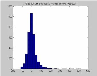
Regardless of the reason, the profits do seem to exist. However, Piotroski (2000) found that most (i.e., 55 to 60%) stocks in value portfolios actually underperformed the market average. This indicates that simple valuation multiples are a crude measure of ‘value’ by themselves; they are poor predictors of high, or other, stock returns. In Figure 1, we present a histogram of the excess one-year returns for all US value stocks over our entire data period (1986 to 2001). This figure shows that the positive return on the value portfolio is driven by a small number of extremely high return stocks, reflected by the strong skew to the right. This paper considers whether it is possible to pre-identify which stocks will reside in either the right and/or left side (relative to 0) of this return distribution, using fundamental company accounting information and a statistical model. Ideally, this would produce an enhanced value portfolio with a higher proportion of stocks that outperform the market, without deleting many (preferably any) of the high return value stocks in the right tail.
Figure 1. Histogram of Excess Returns (% per annum) across All US Value Portfolios, 1986 to 2001 Various papers in the financial literature have attempted to better identify value stocks as truly undervalued using non-statistical models or rules-of-thumb. Asness (1997) showed that momentum provides a good basis for separating out true and false ‘growth’ stocks but that it is much less successful at predicting true and false value stocks. Piotroski (2000) demonstrated that a check-list of 9 accounting variables could be used to rank value stocks successfully. However, this work was
not tested in a true forecast setting; the 9 variables were chosen using the same data that the model was tested upon, partially explaining the highly profitable returns reported. We note that our proposed strategy is a true forecasting strategy and is implementable in a real world investment environment. Beneish et al. (2000) also found that fundamental variables can be useful for identifying stocks whose returns falls in the extreme tails of the return distribution. The approach in this paper is to develop a statistical model for value stocks in the spirit of Ou and Penman (1989), who used 68 accounting variables to build a logistic regression model based on the previous 5 years of earnings performance so as to forecast whether a firms earnings would increase or decrease in subsequent years. The contribution of this paper is thus to examine the extent to which a statistical model and statistical forecasting methods, as opposed to rules-of-thumb, can be used to separate value stocks into those that will rise in price and those that will fall using information in fundamental accounting variables.
Many forecasting studies seek to combine forecasts across models and illustrate clear improvements in forecast accuracy over single model approaches; see for instance Zou and Yang (2004), Min and Zellner (1993), Garratt et al. (2000) and Gneiting and Raftery (2005). The Bayesian approach is via model averaging; see Kass and Raftery (1995), Lewis and Raftery (1997) and Raftery et al. (1997). Applications of these approaches often involve small numbers of competing models; see for example Fernandez et al. (2001). When there are many variables to choose from, it can be intractable to combine every possible model. Model space reduction is necessary in this case. Kass and Raftery (1995) employed Occam’s razor while Stock and Watson (2002) used principal components to reduce the dimensionality. Markov chain Monte Carlo (MCMC) approaches have been suggested to perform model averaging simultaneously with reducing the model space (e.g., see George and McCulloch, 1993, and Smith and Kohn, 1996, for linear regression; Wood and Kohn, 1998, and Gerlach et al. (2002) for binary regression; and Green, 1995, for general discussion). The idea is to design an MCMC sampling scheme that can sample from the posterior density of all possible models. A goal of this paper is to employ a Bayesian model averaging approach, via an MCMC sample, to combine forecasts from competing logistic regression models in order to design an implementable enhancement of a simple value investment strategy.
In this paper we use a large set of lagged accounting variables in a logistic regression, estimated by MCMC methods, and a Bayesian model averaging technique to forecast the probability that value stocks will outperform the market in the next year. We use the previous 5 years of accounting and return data as the data sample. A number of investment strategies using these probability forecasts are then developed, examined and illustrated to add profit to value investment returns. Our findings support the hypothesis that accounting variables can be used as the basis for more successfully identifying undervalued stocks within a value portfolio. These findings provide insights into the usefulness of accounting information, suggest a market inefficiency in that public information can be used to enhance an investment strategy and suggest how managers can supplement their own investment strategies.
In Section 2, we describe our data and methods for ranking value stocks, including model averaging techniques. The investment strategies employed and their performances are reported and discussed in Section 3. Section 4 concludes.
2. Data and Methods
In this section, we describe the data and the methods used to provide forecasts aimed at separating value stocks into those that are likely to outperform the market and those that are likely to underperform. We define value stocks using the book-to-market ratio, as in Piotrovski (2000). We examine three markets: the US, the UK and Australia. A combination of differing market sample sizes and requiring a sufficient sample for estimation means we use a slightly different definition for ‘value’ in each market: the top 25% of stocks, ranked by book-to-market ratio, in the US and the UK and the top 33% in Australia, a much smaller market.
2.1 Fundamental Variables
We did not begin with as large a number of fundamental variables as Ou and Penman (1989) but rather were more selective in the potential variables considered. These are chosen were follows:
1. Variables identified by other work as useful for value stocks (e.g., Beneish et al., 2000; Piotroski, 2000).
2. Variables identified by Bird et al. (2002) as useful for stock performance prediction.
The 23 variables listed in Table 1 were included in the US models; data restrictions meant only including the first 18 for the UK and Australian markets. These variables are publicly available in accounting statements for firms in major markets. Most of this data, including returns, were obtained from the COMPUSTAT databases, with some supplementation from GMO’s proprietary databases. The sample of firms included in each year were composed of all firms in the relevant database, with the exception of financial stocks and those stocks for which we had an incomplete set of fundamental or return data which were deleted.
We use these variables, and an overlapping set of 5-year windows of stock returns, to forecast the direction of stock returns in the value portfolio for each year from 1986 to 2001 (US) and from 1990 to 2001 (UK and Australia). Note that in the US this involves 16 separate statistical analyses, each using only the previous 5 years of sample data, to form the forecasts in the subsequent year, similar to the method of Ou and Penman (1989). We chose this strategy to allow the forecast model to potentially change for each forecast year, with differing effects from each accounting variable allowed in different forecast years, as opposed to the constant rule applied in Piotrovski (2000).
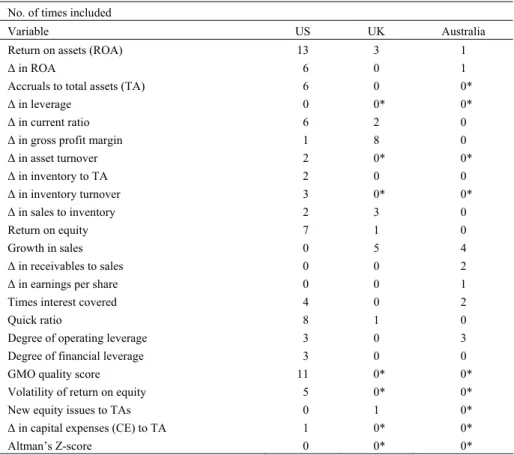
Table 1. Each Variable’s Inclusion in the Most Likely Model. No. of times included
Variable US UK Australia
Return on assets (ROA) 13 3 1
Δ in ROA 6 0 1
Accruals to total assets (TA) 6 0 0*
Δ in leverage 0 0* 0*
Δ in current ratio 6 2 0
Δ in gross profit margin 1 8 0
Δ in asset turnover 2 0* 0* Δ in inventory to TA 2 0 0 Δ in inventory turnover 3 0* 0* Δ in sales to inventory 2 3 0 Return on equity 7 1 0 Growth in sales 0 5 4 Δ in receivables to sales 0 0 2
Δ in earnings per share 0 0 1
Times interest covered 4 0 2
Quick ratio 8 1 0
Degree of operating leverage 3 0 3
Degree of financial leverage 3 0 0
GMO quality score 11 0* 0*
Volatility of return on equity 5 0* 0*
New equity issues to TAs 0 1 0*
Δ in capital expenses (CE) to TA 1 0* 0*
Altman’s Z-score 0 0* 0*
Notes: Δ indicates annual change. * indicates that this data was not available for every year.
The first step is to rank all of the stocks on the basis of their book-to-market value at the start of each financial year in the sample (e.g., April for years 1983 to 2001 in the US) then form the value portfolios, defined above, in each year. In line with the typical financial year, and allowing for a lag in the availability of fundamental data, we build the forecast models as at the beginning of April for both the US and the UK and at the beginning of October for the Australian market. We use a 5-year sample window of data to build forecast models; the exceptions to this are the first 2 forecast years in each market that used only the previous 3 and 4 years of data, respectively. More details of the availability of data for the three markets are provided in Tables 2 and 3.
2.2 Method of Model Development
The returns in the value portfolio are transformed to a binary series, y that record whether stock i has an annual return that is higher than the market return in
year t (yit =1) or a lower return (yit =0). The probability of outperforming the
Pr(yit = =1) πit, i= K1, ,mt, (1)
where mt is the number of stocks in the value portfolio in year t. This probability
is what we will attempt to forecast in our analysis. As in Gerlach et al. (2002), we use the standard logistic link function with random effect:
(
)
(
)
, 1log πit 1−πit =zit =Xi t−β+eit, i=1, ,K mt, (2)
where the errors are independently distributed as ~ (0, 2)
it
e N σ . The row vector
, 1
i t−
X contains the values of the 23 accounting variables for observation (stock) i in year t−1. For example, for the US market in the year 1997 (i.e., April 1996 to March 1997), the accounting variables used in the vectors Xi t, 1− are those available
as at the end of March 1996. This allows us to have the required accounting information available at the time when we make the one-year-ahead forecasts and hence avoids any look-ahead bias in forecasting.
Note that the same subscript i will in general not refer to the same firm in different years, as firms come into and out of the value portfolio from year to year. The model implicitly assumes that return direction depends only on fundamental information and thus any correlation over time for particular stocks is ignored and assumed negligible.
We group the observations and lagged variables y and X into overlapping 5-year windows and perform separate analyses on each sample window to form forecasts of π for each value stock in each year from 1986 to 2001 in the US. it
This allows us to simulate an ongoing investment strategy with annual re-balancing based on the previous 5-years of data. As an example, to forecast y1990 (i.e., the US
value portfolio in 1990), the forecasting model(s) are developed using returns over the 5-year sample period from April 1985 to March 1989 grouped together (y y= 1985, ,K y1989) linked to fundamental variables available in March in the years
1984 to 1988 (X X= 1984, ,K X1988). Investment portfolios are formed annually using
these forecasted probabilities as described in Section 3.
Rather than put all variables directly into the model, we wish to do variable selection and then model average forecasts across the possible models. We favor an MCMC approach to reduce the model space, extending the original stochastic search algorithm of George and McCulloch (1993). This allows efficient traversal of the posterior model space via a posterior sample of possible models. Gerlach et al. (2002) introduced an MCMC technique for a logistic regression model. We can estimate the relative posterior probability for each model using the proportion of times each model is selected in the MCMC sample. This allows us to forecast the probability of outperforming the market using the model averaging approach. The MCMC sampling scheme, model selection and model averaging techniques are outlined below.
2.3 MCMC Variable Selection and Sampling Scheme
auxiliary variables are introduced to indicate which accounting variables are to be included in the model at each iteration, denoted J, where Ji = indicates that the 1
i th variable is to be included and Ji =0 the opposite. The goal is to sample from
the joint posterior density p J y( ). An estimate of p J y( ) is then obtained as the
proportion of times each model was selected in the sample, as in George and McCulloch (1993).
To obtain an MCMC sample from p J y( ), we simulate iteratively from the
conditional densities: (i) p J( i y z J, , ≠i), i= K1, , 23; (ii) p(z y J β, , ,σ2); (iii)
J z, y,
β )
(
p ; (iv) p(σ2 y z J β, , , ). Methods to do this are detailed in Gerlach et al.
(2002). Initial values are randomly chosen for the unknown model parameters and latent variables from their prior distributions. MCMC iterates are then successively generated in turn from each of the posterior distributions (i) to (iv). Typically we run the sampling scheme for 5000 iterations as a warm-up period and then collect samples for the next 20000 iterations.
2.4 Prior Information
Where prior information is available, it can be incorporated into the estimation procedure in the usual way. Successive 5-year windows of data have 4 years overlap and hence are not independent. If, for example, the variable return on assets has a strong effect (i.e., large Pr(Ji = y1 )) over a particular 5-year period, we can incorporate this information into inference for the next 5-year window, commencing with a stronger prior for inclusion of this variable. We use this option when setting the priors (p Ji J≠i) as follows. The rules were based on the posterior probabilities obtained for each accounting variable in the previous 5-year period only. Let y *
refer to the previous 5-year sample, with a 4-year overlap with the current sample window y. The rules are as follows:
1. Set the prior probability Pr(Ji =1J≠i) 0.65= if
* Pr(Ji =1y ) 0.65≥ ; 2. Set Pr( 1 ) Pr( 1 *) i i i J = J≠ = J = y if 0.35 Pr(≤ Ji =1y*) 0.65≤ ; 3. Set Pr(Ji =1J≠i) 0.35= if * Pr(Ji =1y ) 0.35≤ . We could simply have used Pr( 1 *)
i
J = y for each variable from the previous
5-year window as the prior for the next 5-year sample window. However, we felt this was not optimal as variables with very high posterior probabilities (say > 0.95) in the previous period would rarely be dropped from the newly selected model, even if they had negligible effect in the one additional sample year; whereas variables with low posterior probabilities would rarely be selected in the updated model. We consider the method above to be a compromise that will allow changes in the market to be captured relatively quickly while still weighting our results in favor of previously successful or important variables, i.e., prior information.
2.5 Model Averaging
This section shows how to model average the probability forecasts. For each forecast year t , we have an MCMC sample of models J[ ]1, ,J[ ]D
estimates θ[ ]1, ,θ[ ]D
K , where θ=( , ,β zσ ′2) , based on the observed 5-years of
sample data * 5, 1
t− t− =
y y and some explanatory variables * 5, 1
t− t− =
X X . We also have the set of presently available updated explanatory variables Xt−1 that we use
to forecast future observations ( , ,1 )
t
t = yt ym t
y K , where m is the number of t
value stocks in year t . The Bayesian model averaging approach is:
(
* *)
(
*) (
* *)
1 Pr it 1 , T Pr it 1 , j Pr j , j y y M M = = y X =∑
= X y X , (3)where M represents each possible model and T is the total number of possible j
models. We can estimate Pr( *, *)
j
M y X as being proportional to its respective
number of times included in the MCMC sample of models. Thus the model averaged forecasted probability of outperforming is:
(
)
(
(
(
, 1 [ ][ ])
)
)
5, 1 6, 1 1 , 1 exp 1 Pr 1 , 1 exp j D i t it t t t t j j i t y D − − − − − = − = ≈ +∑
X β y X X β . (4)To summarise, the forecasts of the probability that each value stock in the subsequent year t will outperform the market average are obtained as below. For
each MCMC iteration:
1. A particular model (Mj) is sampled.
2. Regression coefficients are sampled conditional upon the model chosen in (1) and the 5-year sample data.
3. The chosen model and parameter values in (1) and (2) are then used to generate probability forecasts for each value stock using (4).
This process of choosing a model, estimating coefficients and generating probability forecasts is repeated for 25,000 MCMC iterations. At the end of the sampling run, we use the last 20,000 forecasted probabilities for each value stock to obtain a model-averaged forecast as in (4). This analysis is repeated for each year in the US from 1986 to 2001.
3. Results
3.1 Effects of Variables
The model averaging procedure results in every accounting variable having some impact, however small, in forecasting the probabilities for each value stock. To investigate the important variables, Table 1 contains the number of years each variable is included in the most likely model. For the US models, 17 of the 23 variables are included at least once (out of 16 forecast years), with each year’s model including 5 to 6 variables on average. The number of variables included varies between 2 and 7 each
year, while 7 variables were in at least 6 out of the 16 models. The most common were return on assets (ROA, 13 years), GMO quality score (11 years), quick ratio (QR, 8 years), return on equity (ROE, 7 years), change in ROA (Δ in ROA, 6 years), change in current ratio (Δ in CR, 6 years) and accruals (6 years). These variables represent a mixture of indicators of the earnings power of the company (ROA, ROE and Δ in ROA) and of short and long-term financial strength (QR, Δ in CR, accruals and GMO quality score).
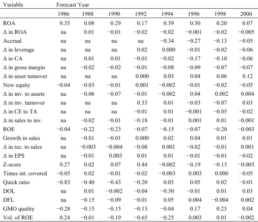
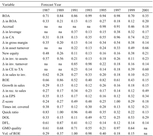
Table 2 shows the model averaged regression coefficient estimates for each variable (standardised) in each even forecast year, while Table 3 shows the posterior probability for model inclusion in odd forecast years. Note the time patterns here: variables can have different effects in different time periods, but there is a clear pattern in their size and direction, as expected. We investigated applying the same model each year, composed of the overall best six variables in our study as listed above, but its ability to generate positive returns was inferior to the approach used in this paper.
Table 2. Coefficients for Each Accounting Variable in Each Even Forecast Year for the US.
Variable Forecast Year
1986 1988 1990 1992 1994 1996 1998 2000 ROA 0.35 0.08 0.29 0.17 0.39 0.30 0.20 0.07 Δ in ROA na 0.01 −0.01 −0.02 −0.02 −0.001 −0.02 −0.005 Accrual na na na na −0.34 −0.27 −0.13 −0.05 Δ in leverage na na na 0.02 0.000 −0.01 −0.02 −0.06 Δ in CA na 0.01 0.01 −0.01 −0.02 −0.17 −0.10 −0.06 Δ in gross margin na −0.02 −0.02 −0.01 −0.08 −0.09 −0.07 −0.07 Δ in asset turnover na na na 0.000 0.03 0.04 0.06 0.12 New equity −0.04 −0.03 −0.01 0.001 −0.002 −0.01 −0.02 −0.05 Δ in inv. to assets na −0.06 −0.07 −0.01 −0.002 0.04 0.002 0.004 Δ in inv. turnover na na na 0.33 0.01 −0.03 −0.07 0.03 Δ in CE to TA na na na −0.01 0.01 −0.001 −0.05 −0.02 Δ in sales to inv. na −0.02 −0.01 −0.18 −0.01 0.001 0.01 −0.001 ROE −0.04 −0.22 −0.23 −0.07 −0.15 −0.07 −0.20 −0.003 Growth in sales na −0.01 −0.01 0.000 0.02 0.04 0.01 0.01 Δ in rec. to sales na −0.003 −0.004 −0.08 0.001 −0.02 −0.01 0.001 Δ in EPS na −0.01 0.003 0.01 0.01 −0.01 −0.01 −0.02 Z-score 0.27 0.02 0.07 0.44 −0.002 −0.19 −0.13 −0.003
Times int. covered −0.05 0.02 −0.01 −0.02 −0.003 0.003 0.000 −0.05
Quick ratio −0.83 −0.40 −0.43 −0.20 0.03 0.05 0.02 −0.01
DOL na 0.01 −0.002 −0.04 −0.30 −0.01 0.01 0.03
DFL na −0.15 −0.09 −0.01 0.05 0.004 −0.004 0.002
GMO quality −0.28 −0.15 −0.15 −0.13 −0.04 0.17 0.23 0.04
Vol. of ROE 0.24 −0.01 −0.19 −0.65 −0.25 0.003 0.01 −0.002
Table 3. Posterior Probability of Inclusion for Each Accounting Variable in Each Odd Forecast Year for the US.
Variable Forecast Year
1987 1989 1991 1993 1995 1997 1999 2001 ROA 0.71 0.84 0.86 0.99 0.94 0.98 0.70 0.35 Δ in ROA 0.33 0.21 0.13 0.15 0.27 0.18 0.12 0.20 Accrual na na na na 0.98 0.91 0.46 0.18 Δ in leverage na na 0.37 0.13 0.15 0.38 0.32 0.17 Δ in CA 0.31 0.18 0.13 0.35 0.55 0.96 0.74 0.22 Δ in gross margin 0.35 0.20 0.13 0.14 0.34 0.54 0.38 0.14 Δ in asset turnover na na 0.22 0.13 0.24 0.33 0.49 0.66 New equity 0.48 0.26 0.11 0.13 0.16 0.16 0.38 0.21 Δ in inv. to assets 0.57 0.56 0.21 0.13 0.18 0.26 0.11 0.23 Δ in inv. turnover na na 0.85 0.98 0.22 0.18 0.16 0.14 Δ in CE to TA na na 0.23 0.14 0.14 0.18 0.39 0.60 Δ in sales to inv. 0.62 0.28 0.27 0.33 0.20 0.18 0.10 0.23 ROE 0.66 0.86 0.52 0.40 0.82 0.61 0.43 0.15 Growth in sales 0.29 0.15 0.12 0.12 0.26 0.16 0.18 0.15 Δ in rec. to sales 0.27 0.17 0.34 0.23 0.17 0.14 0.12 0.49 Δ in EPS 0.35 0.15 0.17 0.12 0.16 0.12 0.32 0.34 Z-score 0.24 0.27 0.49 0.48 0.25 1.00 0.29 0.18
Times int. covered 0.38 0.17 0.12 0.30 0.28 0.13 0.32 0.21
Quick ratio 0.83 1.00 0.96 0.48 0.35 0.32 0.22 0.13
DOL 0.33 0.15 0.11 0.49 0.72 0.25 0.53 0.29
DFL. 0.61 0.87 0.41 0.12 0.14 0.12 0.14 0.14
GMO quality 0.61 0.68 0.71 0.55 0.21 0.97 0.64 na
Vol. of ROE 0.29 0.37 1.00 0.98 0.40 0.18 0.15 na
Only 8 variables prove to be important in one or more UK model years; on average there are only 3 important variables in any year. Only two variables are included in more than 50% of the UK models (change in gross profit margin is in all 8 models; growth in sales is in 5). In the case of Australia, 7 variables appeared at least once out of 7 years, with on average only 2 variables included each year. Growth in sales (4 models) and degree of operating leverage (3 models) are the most popular, with only the former a consistently important variable in the UK models. There is really no evidence of any consistency across markets in the variables having a strong influence on value stocks. While these variables do continue the theme of profitability and financial strength being important for the subsequent performance of value stocks, the lack of consistency across different markets remains an issue for further study.
3.2 Investment Strategies: The US Models and Returns
Using the P-values (the forecasted probabilities of outperforming), the two investment strategies we consider are:
1. Rank stocks in terms of their P-value, then invest in the top quartile (top25%) or bottom quartile (bot25%).
2. Invest in those value stocks which have a P-value greater than 0.6 (P>0.6)
and those value stocks with a P-value less than 0.4 (P<0.4), as in Ou and
Penman (1988).
We note that the first strategy generally allows investment in more stocks than the second strategy, as in some years only a few stocks have a forecasted P>0.6.
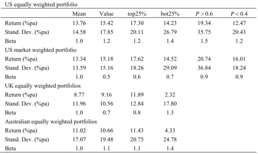
The performance of these strategies for both equally weighted and market weighted portfolios are summarised in Table 4. This contains annualised returns (i.e., a geometric mean) over the 16 year forecasting period, based on each strategy above, the value portfolio and the whole market. Both our proposed strategies provide a reasonable separation of the good value stocks (either top25% or P>0.6) and the
poor value stocks (bot25% or P<0.4), for both equally weighted and market
weighted portfolios. The top25% strategy approximately doubles the added value of the standard value strategy and outperforms the bot25% portfolio by approximately 3% per annum (PA) in a long versus short strategy. The P>0.6 strategy triples the
added value of the value strategy and achieves an even greater separation from the
4 . 0 <
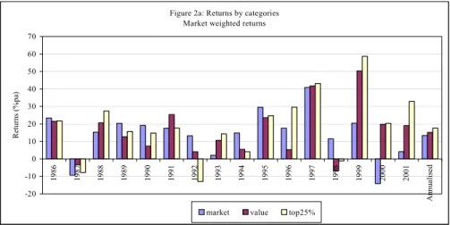
P strategy. Figure 2 (2a) compares the annual equally (market) weighted
returns on the market, the value portfolio and the top25% strategy. Both figures illustrate the comparative higher return of the top25% strategy in most years.
Table 4. Return and Risk Associated with Alternative US Investment Strategies. US equally weighted portfolio
Mean Value top25% bot25% P>0.6 P<0.4
Return (%pa) 13.76 15.42 17.30 14.23 19.34 12.47
Stand. Dev. (%pa) 14.58 17.85 20.11 26.79 35.75 20.43
Beta 1.0 1.2 1.2 1.4 1.5 1.2
US market weighted portfolio
Return (%pa) 13.34 15.18 17.62 14.52 20.74 16.01
Stand. Dev. (%pa) 13.59 15.16 18.26 29.09 36.84 18.24
Beta 1.0 0.5 0.6 0.7 0.9 0.9
UK equally weighted portfolios
Return (%pa) 8.77 9.16 11.89 2.32
Stand. Dev. (%pa) 11.96 10.56 12.84 17.80
Beta 1.0 0.7 0.8 1.3
Australian equally weighted portfolios
Return (%pa) 11.02 10.66 11.43 4.33
Stand. Dev. (%pa) 17.07 19.48 20.75 24.78
Beta 1.0 1.1 1.1 1.4
Figure 2 : Returns by categories Equally weighted returns
-30 -20 -10 0 10 20 30 40 50 60 70 1986 1987 1988 1989 1990 1991 1992 1993 1994 1995 1996 1997 1998 1999 2000 2001 A nnua lis ed R et urn s (% pa )
market value top25%
Figure 2. Comparison of Annual Returns: Equally Weighted.
Figure 3. Comparison of Annual Returns: Market Weighted. 3.3 Risk
The superior performance of the P>0.6 strategy as compared to the top25%
strategy comes at the cost of more highly concentrated and riskier portfolios, as can be seen in Table 4 using the standard risk measures: return standard deviation and market Beta. This suggests that differential risk across the various portfolios may at least partially explain some of the variation in performance, particularly of the equally weighted portfolios. However, the added value of our strategies is unlikely
Figure 2a: Returns by categories Market weighted returns
-20 -10 0 10 20 30 40 50 60 70 19 86 19 87 19 88 19 89 19 90 19 91 19 92 19 93 19 94 19 95 19 96 19 97 19 98 19 99 20 00 20 01 A nnu al is ed Ret ur ns (%p a)
to be fully explained by this risk.
In the remainder of the discussion of the performance of the US models, we concentrate on the top25% strategy. Figure 2 shows that the top25% strategy outperforms the value portfolio in 12 of the 16 years, with most of the poor performance coming in the early 1990s. Tables 2 and 3 show that a major change occurred in 1994: a number of variables with strong effects up to that date (e.g., the quick ratio and the change in inventory turnover) diminish in importance, being replaced by strong effects from other variables (e.g., accruals and change in liquidity). The worst performance seemingly came at the end of one model ‘regime’ and then improved markedly with the new models. This suggests that the model averaging procedure may react slowly to changes in the markets over time. In response, we applied both a 2-year and a 3-year window to generate forecasts in all years. However, this resulted in lower returns over the period. Another option is increasing the frequency of re-balancing the portfolio from annual to quarterly. Although this may be possible within the US market, it is not in other markets, where information on the explanatory variables only becomes available once a year. 3.4 Less Concentrated Strategies
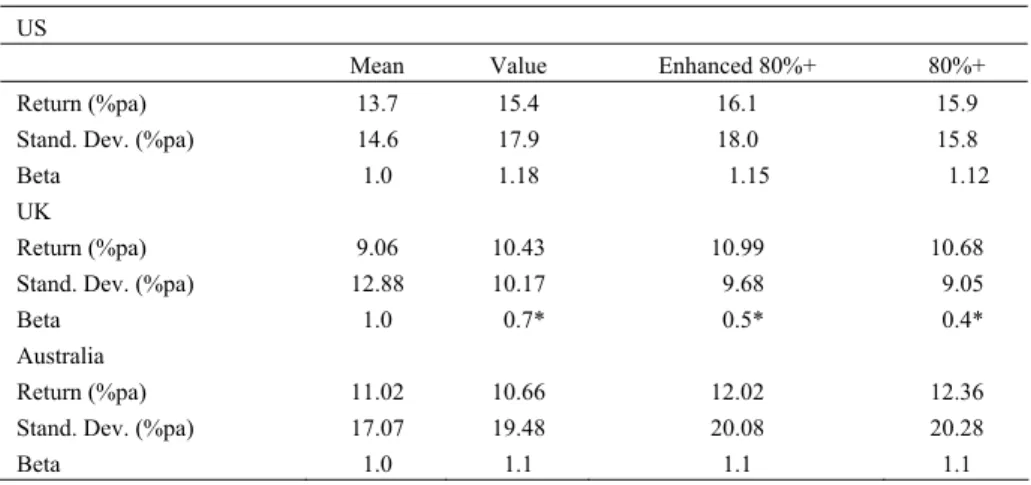
The strategies considered to date involved concentrated portfolios (e.g., average holding of less than 60 stocks in the US, 25 in the UK and 13 in Australia). We further investigated two alternative, more diverse portfolios:
1. 80%+, where the bottom quintile of stocks is dropped from the value portfolio.
2. Enhanced 80%+, where the bottom quintile of value stocks is dropped from the portfolio and the top quintile is given a double weighting in the investment portfolio.
The performance for US stocks is reported in Table 5. The enhancements to the value returns from these strategies are 0.5 to 0.7%pa for the 16-year period. Although this is small in absolute terms, it represents about a 50% addition to the added value achieved by the value portfolio over the market and comes at an apparently reduced level of risk. The source of the additional added value is fairly equally split between over-weighting the value stocks with P-values in the top quintile and avoiding investing in those value stocks with P-values in the bottom quintile. We also investigated substituting 90% for 80%; the results were positive in return but not as consistent nor as strong as those reported for the 80% strategies. 3.5 Sources of Improved Performance
The original problem with value strategies is that the majority of value stocks underperform the market. One objective was to increase the proportion of stocks that outperform the market: results are shown in Table 7. The success rate of the top25% portfolios is 4% above that of the value portfolio, while that of the bot25% portfolio is 3% below the value strategy. These proportions are not independent, as one is a
subset of the other. Using a bootstrap re-sampling method on the value stocks, these observed differences were found to be significant at the 5% level. Further, the bot25% strategy is correct 59% of the time, significantly greater than 50% at the 1% level, in picking stocks that will underperform the average market return.
Table 5. Performance of Less Concentrated Value Strategies. US
Mean Value Enhanced 80%+ 80%+
Return (%pa) 13.7 15.4 16.1 15.9
Stand. Dev. (%pa) 14.6 17.9 18.0 15.8
Beta 1.0 1.18 1.15 1.12
UK
Return (%pa) 9.06 10.43 10.99 10.68
Stand. Dev. (%pa) 12.88 10.17 9.68 9.05
Beta 1.0 0.7* 0.5* 0.4*
Australia
Return (%pa) 11.02 10.66 12.02 12.36
Stand. Dev. (%pa) 17.07 19.48 20.08 20.28
Beta 1.0 1.1 1.1 1.1
Notes: * indicates significantly different from 1.
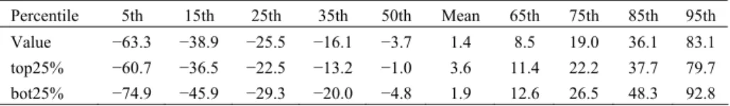
The percentiles of the distribution of excess returns for the whole 16-year value portfolio (see Figure 1), the top25% and bot25% portfolios are presented in Table 6. This clearly shows that the value distribution has been pushed to the right (except in the extreme right tail) by the top25% selection strategy. Similarly, the bot25% portfolio pushes the value portfolio distribution generally to the left (negative). The value portfolio typically sits right in the middle of the percentiles for the top25% and bot25% strategies. Surprisingly, the bot25% portfolio does best in the extreme right tail, perhaps reflecting the increased risk of this portfolio. The top25% strategy thus avoids investing in a number of subsequently poor performing value stocks, without sacrificing many (although unfortunately not all) of the very good value stocks. 3.6 The UK and Australian Models
Both the UK models and the Australian models produce enhanced value portfolios which perform at least as well as if not better than the US portfolios, as illustrated in Table 4. In the case of the UK, the top25% portfolio adds in excess of 2.5%pa to the performance of the value portfolio while a long/short portfolio based on the top25% and the bot25% earns almost 10%pa. Further, this added value is achieved without any significant increase in total risk and at a level of market risk less than 1. The improved performance in Australia is slightly less than for the UK, with the top25% strategy enhancing the return on value by about 0.75%pa and the long/short strategy based on the top25% and the bot25% returning 7%pa. Again, this improved performance comes without any significant increase in risk.
Table 6. Percentiles of Excess Return Distribution in the US.
Percentile 5th 15th 25th 35th 50th Mean 65th 75th 85th 95th
Value −63.3 −38.9 −25.5 −16.1 −3.7 1.4 8.5 19.0 36.1 83.1
top25% −60.7 −36.5 −22.5 −13.2 −1.0 3.6 11.4 22.2 37.7 79.7
bot25% −74.9 −45.9 −29.3 −20.0 −4.8 1.9 12.6 26.5 48.3 92.8
Table 7. Proportion of Stocks Outperforming the Market.
US UK Australia
Value 0.44 0.45 0.40
top25% 0.48* 0.47 0.44
bot25% 0.41* 0.39 0.35
Notes: * indicates significantly difference with the corresponding value portfolio proportion. For the US, improved performance seemed largely due to improving identification of those value stocks that would outperform the market over the next 12 months. Similar evidence for the UK and Australian strategies are also reported in Table 7. The evidence supports the proposition that much of the improved performance of the proposed value strategies has been due to being able to differentiate between the good and bad value stocks. Finally, we applied the same less concentrated strategies to the UK and Australian markets as to US stocks, with results shown in Table 5. For the UK, the improvements in performance are small but are achieved with an overall reduction in risk. For Australia, the improvement in performance over the value portfolio are a significant 1.5%pa, which comes entirely from the deletion of the bottom quintile of value stocks based on our probability estimates and involve only a very small increase in portfolio risk.
4. Conclusion
In this paper we use a logistic regression setting with model averaging across a large number of potential models to enhance a forecast value investment strategy applied to stock markets in the US, the UK and Australia. The hypothesis in this paper was that the stocks in the value portfolio that are most likely to show positive market-corrected returns can be predicted more successfully through the use of fundamental company accounting information. From the results, it appears this is indeed the case but that the sources of accounting data that most influence stock performance seem to vary both across time and across markets.
References
Asness, C., (1997), “The Interaction of Value and Momentum Strategies,” Financial
Analysts Journal, 53, 29-37.
Basu, S., (1977), “Investment Performance of Common Stocks in Relation to Their Price-Earnings Ratio,” Journal of Finance, 32, 663-682.
Beneish, M., C. Lee and R. Tarpley, (2001), “Contextual Fundamental Analysis through the Prediction of Extreme Returns,” Review of Accounting Studies, 6, 165-189.
Bernard, V., J. Thomas and J. Wahlen, (1997), “Accounting-Based Stock Price Anomalies: Separating Market Inefficiencies from Risk,” Contemporary
Accounting Research, 14, 89-136.
Chan, K., Y. Hamao and J. Lokonishok, (1991), “Fundamentals and Stock Returns in Japan,” Journal of Finance, 46, 1739-1764.
Dreman, D. and M. Berry, (1995), “Analysts Forecasting Errors and Their Implications for Security Analysis,” Financial Analysts Journal, 51, 30-41. Fama, E. and K. French, (1992), “The Cross-Section of Expected Stock Returns,”
Journal of Finance, 47, 427-465.
Fernandez, C., E. Ley and M. Steel, (2001), “Model Uncertainty in Cross-Country Growth Regressions,” Econometrics, No. 0110002, Economics Working Paper Archive at WUSTL.
Garratt, A., K. C. Lee, M. H. Pesaran and Y. Shin, (2000), “Forecast Uncertainties In Macroeconometric Modelling: An Application to the UK Economy,” CESifo
Working Paper, No. 345.
George, E. and R. McCulloch, (1993), “Variable Selection via Gibbs Sampling,”
Journal of the American Statistical Association, 88, 881-889.
Gerlach, R., R. Bird and A. Hall, (2002), “Bayesian Variable Selection in Logistic Regression: Predicting Company Earnings Direction,” Australian and New
Zealand Journal of Statistics, 44(2), 155-168.
Gneiting, T. and A. E. Raftery, (2005), “Weather Forecasting with Ensemble Methods,” Science, 310, 248-249.
Graham, B., D. Dodd and S. Cottle, (1962), Securities Analysis: Principles and
Techniques, 4th ed., McGraw-Hill.
Kass, R. and A. Raftery, (1995), “Bayes Factors,” Journal of the American
Statistical Association, 90, 773-795.
Lakonishok, J., A. Shleifer and R. Vishny, (1994), “Contrarian Investment, Extrapolation, and Risk,” The Journal of Finance, 49, 1541-1578.
Lewis, S. and A. Raftery, (1997) “Estimating Bayes Factors via Posterior Simulation with the Laplace-Metropolis Estimator,” Journal of the American Statistical
Association, 92, 648-655.
Min, C. K. and A. Zellner, (1992), “Bayesian and Non-Bayesian Methods for Combining Models and Forecasts with Applications to Forecasting International Growth Rates,” California Irvine—School of Social Sciences
Working Papers, No. 90-92-23.
Mira, A. and L. Tierney, (2002), “Efficiency and Convergence Properties of Slice Samplers,” Scandinavian Journal of Statistics, 29, 1-12.
Ou, J. and S. Penman, (1989), “Financial Statement Analysis and the Prediction of Stock Returns,” Journal of Accounting and Economics, 11, 295-329.
Piotroski, J., (2000), “Value Investing: The Use of Historical Financial Statement Information to Separate Winners from Losers,” Journal of Accounting
Research, 38, 1-41.
Raftery, A., (1996) “Approximate Bayes Factors and Accounting for Model Uncertainty in Generalised Linear Models,” Biometrika, 83, 251-266.
Raftery, A., D. Madigan and J. A. Hoeting, (1997), “Bayesian Model Averaging for Linear Regression Models,” Journal of the American Statistical Association, 92, 179-191.
Rosenberg, B., K. Reid and R. Lanstein, (1985), “Persuasive Evidence of Market Inefficiency,” Journal of Portfolio Management, 11, 9-17.
Rouwenhorst, G., (1999), “Local Return Factors and Turnover in Emerging Markets,” The Journal of Finance, 54, 1439-1464.
Stock, J. and M. Watson, (2002), “Forecasting Using Principal Components from a Large Number of Predictors,” Journal of the American Statistical Association, 97, 1167-1179.
Smith, M. and R. Kohn, (1996), “Nonparametric Regression Using Bayesian Variable Selection,” Journal of Econometrics, 75(2), 317-343.
Zou, H. and Y. Yang, (2004), “Combining Time Series Models for Forecasting,”