應用最佳節能位置上傳機制之研究於行動計算環境

國 立 交 通 大 學

電信工程研究所

碩 士 論 文

Optimal Energy-Efficient Location Update

for Mobile Computing

應用最佳節能位置上傳機制之研究

於行動計算環境

研究生：張凱評

指導教授：王蒞君 教授

應用最佳節能位置上傳機制之研究於行動計算環境

Optimal Energy-Efficient Location Update for

Mobile Computing

研 究 生：張凱評 Student：Kai-Ping Chang

指導教授：王蒞君 Advisor：Li-Chun Wang

國 立 交 通 大 學

電信工程研究所

碩 士 論 文

Submitted to Institute of Communications Engineering College of Electrical and Computer Engineering

National Chiao Tung University in partial Fulfillment of the Requirements

for the Degree of Master of Science

In

Communications Engineering August 2011

Hsinchu, Taiwan, Republic of China

應用最佳節能位置上傳機制之研究於行動計算環境

學生：張凱評

指導教授：王蒞君

國立交通大學

電機學院電信工程研究所

摘要

提供適地性服務 (Location-Based Services, LBSs) 的最關鍵議題之一，是

行動終端裝置因位置的頻繁更新需求所造成的耗電 (Power Consumption) 問

題。在本篇論文中，我們提出一個電源感知的位置上傳機制 (Power-Aware

Location Update Scheme) ， 另 稱 作 基 於 能 量 考 量 的 位 置 回 傳 方 法

(Energy-Based Location Reporting) 。 本 論 文 應 用 動 態 規 劃 (Dynamic

Programming, DP) 於 傳 統 的 距 離 考 量 位 置 回 傳 方 法 (Distance-Based

Location Reporting) ， 決 定 最 佳 節 能 位 置 上 傳 (Optimal Energy-Efficient

Location Update) 機制，使得在行動計算 (Mobile Computing) 環境中，達成

降低耗電的目標。提出基於動態規劃下 (DP-Based) 的位置上傳機制，容許

位置回傳錯誤 (Location Reporting Errors) 在令人滿意的範圍內。我們也在不

同的能量比率 (Energy Ratio) 與不同的終端移動速度 (Terminal Moving

Speed) 下，驗證提出的最佳節能位置上傳機制。

Optimal Energy-Efficient Location Update

for Mobile Computing

A THESIS Presented to

The Academic Faculty By

Kai-Ping Chang

In Partial Fulfillment

of the Requirements for the Degree of Master in Communications Engineering

Institute of Communications Engineering College of Electrical and Computer Engineering

National Chiao Tung University

2011

Abstract

One of the most critical issues in providing location-based service is the power consumption in mobile terminals due to frequent location queries. In this thesis, we present a power-aware location update scheme, called energy-based location reporting. We apply dynamic programming (DP) to the traditional distance-based location reporting method to determine the optimal location update scheme with an objective of minimizing power consumption in mobile computing. The proposed DP-based energy-efficient location update scheme can also tolerate the location reporting errors within a satisfied level. We also verify the optimal location update scheme by simulations for different energy ratios and different terminal moving speeds.

Acknowledgements

I would like to thank my parents and my older brother. They always give me endless supports. I especially thank Professor Li-Chun Wang who gave me many valuable suggestions in my research during these two years. I would not finish this work without his guidance and comments.

In addition, I am deeply grateful to my laboratory mates, Chu-Jung, Ang-Hsun, I-Cheng, Wei-Ping, Chien-Cheng, Yu-Jung, Tsung-Ting, and junior laboratory mates at Mobile Communications and Cloud Computing Labra-tory at the Graduate Institute of Communications Engineering in National Chiao-Tung University. They provide me with a lot of assistance and share happiness with me.

Contents

Abstract i

Acknowledgements ii

Contents iii

List of Tables vi

List of Figures vii

1 Introduction 1

1.1 Problem and Solution . . . 4

1.1.1 Optimal Energy-Efficient Location Update . . . 5

1.2 Thesis Outline . . . 5

2 Background 6 2.1 Literature Survey . . . 6

2.1.1 Time-Based Location Reporting Scheme . . . 7

2.1.2 Distance-Based Location Reporting Scheme . . . 8

2.2 Dynamic Programming . . . 9

3 System Models 20

3.1 System Architecture . . . 20

3.2 Hovering Around Border Effects . . . 23

3.3 Performance Metrics . . . 24

3.3.1 Average Power Consumption P = Pc+ Pr . . . 24

3.3.2 Average Location Error Le . . . 25

3.3.3 Maximum Location Error Le max . . . 25

4 Proposed Energy-Efficient Location Update Mechanism 27 4.1 Assumptions . . . 27 4.2 Definitions . . . 28 4.2.1 System States . . . 28 4.2.2 Action Representations . . . 33 4.2.3 Transition Probabilities . . . 33 4.2.4 Cost Functions . . . 35

4.3 Optimal Energy-Efficient Location Update Algorithm . . . 37

4.3.1 Principle of Optimality . . . 37

4.3.2 Procedures of Power Consumption Minimization . . . . 38

5 Numerical Results 41 5.1 Simulation Setup . . . 41

5.2 Effects of Energy Ratio on Power Consumption for Various Lo-cation Update Schemes with Different Terminal Moving Speeds 42 5.3 Effects of Terminal Moving Speeds on Location Errors for Var-ious Location Update Schemes with Different Energy Ratios . 48 6 Conclusions 58 6.1 Energy-Efficient Location Update Mechanism . . . 58

Bibliography 61

List of Tables

2.1 Comparison of Various Schemes for Location Updates. . . 7

4.1 The System Parameters for Illustration. . . 30

4.2 All States. . . 33

List of Figures

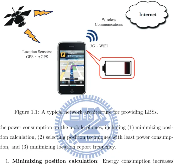
1.1 A typical network architecture for providing LBSs. . . 2

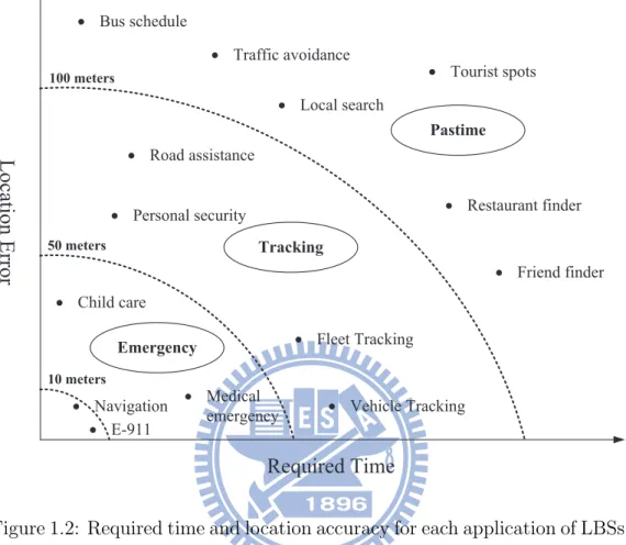
1.2 Required time and location accuracy for each application of LBSs. . . 4

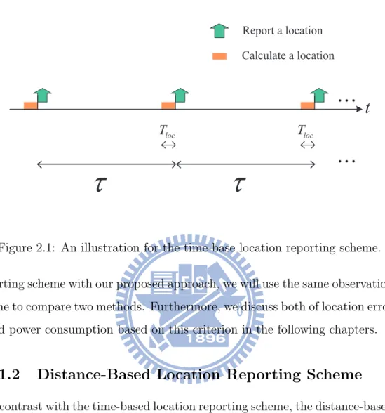
2.1 An illustration for the time-base location reporting scheme. . . 8

2.2 An illustration for the distance-base location reporting scheme. 10 2.3 A topology for the shortest-path problem. . . 11

2.4 Backward recursion for solving the shortest-path problem. . . 14

2.5 Forward recursion for solving the shortest-path problem. . . . 14

2.6 The sequential decision making model. . . 16

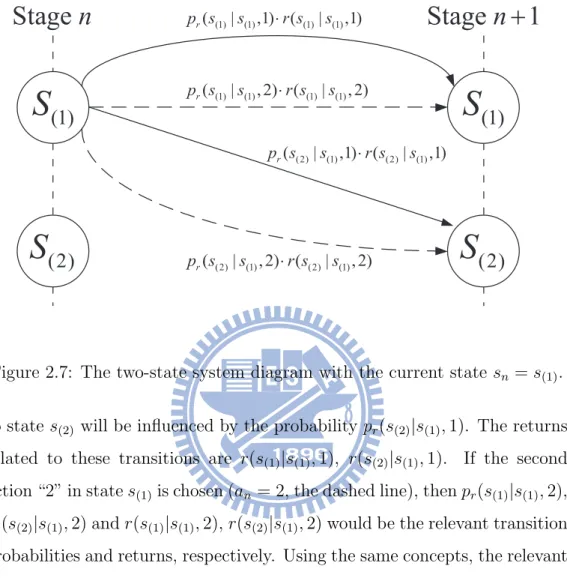
2.7 The two-state system diagram with the current state sn = s(1). 17 2.8 The two-state system diagram with the current state sn = s(2). 18 3.1 The system architecture. . . 21

4.1 An illustrative example of stochastic system. . . 29

4.2 The state illustration based on system parameters. . . 31

4.3 The state transition diagrams. . . 32

4.4 An illustrative example of calculating the transition probability. 36 4.5 The flow chart of optimal energy-efficient location update al-gorithm. . . 40

5.1 Effects of the energy ratio on the overall system power con-sumption for various location update schemes with different terminal moving speeds. . . 47 5.2 Effects of the terminal moving speed on average location errors

for various location update schemes with different energy ratios. 52 5.3 Effects of the terminal moving speed on maximum location

er-rors for various location update schemes with different energy ratios. . . 56

Chapter 1

Introduction

Location-based services (LBSs) provide real-time services with user’s lotions [1–3]. Because current mobile devices have location calculation ca-pability, the LBSs have gained a lot attention over the past years. Some examples of LBSs include providing local information, such as traffic notifi-cation, stores, and spots. Another key feature of in recent is related to social networks [4]. A user can obtain the local information based on his current location, and share his local information (e.g. restaurants, shops and tourist spots) with community members.

Even though mobile devices provide the convenience of ubiquitous com-putations, the use of mobile devices is severely constrained by the limited battery capacity. Thus, it is important to minimize the power consump-tion of these energy-constrained mobile devices. Figure 1.1 shows a typi-cal network architecture for providing LBSs, consisting of location update mechanisms and wireless communications. Consequently, LBSs consume the energy Ec required for calculating a location, and the energy Er of reporting a location [5]. According to [6], Ec is usually higher than Er.

Wireless Communications

3G_ˣWiFi Location Sensors:

GPS_ˣAGPS

Figure 1.1: A typical network architecture for providing LBSs.

the power consumption on the mobile phones, including (1) minimizing posi-tion calculaposi-tion, (2) selecting posiposi-tion techniques with least power consump-tion, and (3) minimizing location report frequency.

1. Minimizing position calculation: Energy consumption increases with the frequency of location calculation. Thus, reducing redundant location calculation can save power. However, location errors become large when the frequency of location report is reduced. In [8], the cache-based approach was proposed to estimate when the application server needs to obtain a new location from a mobile device. As long as location errors are lower than tolerant value, the latest cached location can be used for LBSs.

2. Selecting position techniques with least power consumption: Different location sensors (e.g. GPS, WiFi, and 3G cellular) yields

different power consumption, and have different tolerant location errors in providing LBSs. In [9], it is suggested that the system can choose the appropriate location sensor to save power. For example, if a mobile device stays within the GSM cell, GPS can be switched off.

3. Minimizing location report frequency: Reducing the report of location frequency can also save power in mobile devices. Basically, there are two kinds of location reporting mechanisms: (1) the

time-based location reporting (TBLR) scheme [10–12], and (2) the distance-based location reporting (DBLR) scheme [5]. For the TBLR scheme, a

moving user sends location information to the server at a fixed time interval. For the DBLR scheme, the moving user sends location in-formation to the server whenever it moves a certain distance. Various location update schemes are suitable for different scenarios. The power consumption of the TBLR and DBLR schemes are affected by differ-ent factors. For the TBLR scheme, the energy ratio Er/Ec affects the power consumption of mobile devices because this scheme requires calculating and reporting locations every fixed period. However, the location calculation periods of mobile locations affect the overall power consumption of the DBLR scheme.

In this thesis, we propose to consider both the factors of location calcu-lation and reporting in the location update mechanism design to minimize the power consumption of mobile devices in LBSs.

On the other hand, location accuracy is also an important factor for LBSs. Figure 1.2 shows that different applications of LBSs require different location accuracy [13]. For example, it usually requires about 80 meters (a minimum city block distance [14]) location accuracy for location-based social networks. Hence, we must consider the location accuracy in our design mechanism. In

Tracking Emergency Pastime · Friend finder · Restaurant finder · Local search · Traffic avoidance · Bus schedule · Tourist spots · Vehicle Tracking · Fleet Tracking · Personal security · Road assistance 50 meters 100 meters 10 meters · Medical emergency · Child care · Navigation · E-911

Lo

cati

o

n

Er

ro

r

Required Time

Figure 1.2: Required time and location accuracy for each application of LBSs. this thesis, we will focus on the LBSs such as location-based social networks to design an energy-efficient location update mechanism.

1.1

Problem and Solution

The objective of this thesis is to develop an energy-efficient location up-date mechanism for mobile devices to support LBSs. An introduced before, TBLR and DBLR schemes focus on reducing the frequency of reporting mo-bile location. To further save energy of momo-bile devices in LBSs, we suggest an energy-efficient location update mechanism needs not only change the frequency of location calculation, but the frequency of location report.

1.1.1

Optimal Energy-Efficient Location Update

In order to minimize the power consumption in mobile terminal for provid-ing LBSs, we investigate how to energy-efficiently change the frequency of location calculation and location report. We present a power-aware location update scheme, called energy-based location reporting method. The pro-posed energy-based location reporting method applies dynamic programming in traditional distance-based location reporting method to determine the op-timal energy-efficient location update. Based on dynamic programming, our proposed location update scheme can not only decide the optimal frequency of location calculation, but the optimal frequency of location report. Because the frequency of location calculation and report are energy-efficiently opti-mized, the power consumption in mobile devices can be minimized. On the other hand, the dynamic-programming based energy-efficient location update scheme can also tolerate the location reporting errors within a satisfied level.

1.2

Thesis Outline

The rest of this thesis is organized as follows. Chapter 2 introduces the background of our proposed approach. Then, we discuss system models and performance metrics in Chapter 3. Subsequently, we present the pro-posed dynamic-programming-based energy-efficient location update scheme in Chapter 4. Numerical results are shown in Chapter 5. Finally, we conclude this thesis in Chapter 6.

Chapter 2

Background

In this chapter, we firstly survey related works to location update schemes in mobile computing. Then, the core concept, “dynamic programming,” for solving the optimization problem applied in our proposed approach is introduced in depth.

2.1

Literature Survey

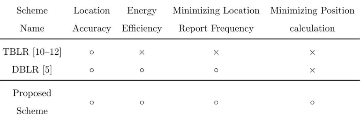
Nowadays, tracking schemes for mobile devices in mobile computing are stud-ied. In this part, we introduce two traditional location reporting schemes, including (1) the time-based location reporting (TBLR) scheme and (2) the distance-based location reporting (DBLR) scheme. However, these location update schemes have not simultaneously considered all of the four design fea-tures. Table 2.1 classifies the existing location reporting techniques, where the signs “◦ ” and “ × ” indicate that the proposed scheme “does” and “does not” consider the corresponding feature, respectively. Furthermore, we il-lustrate the concepts of both schemes briefly and highlight what literature exploits the above schemes.

Table 2.1: Comparison of Various Schemes for Location Updates.

Scheme Location Energy Minimizing Location Minimizing Position

Name Accuracy Efficiency Report Frequency calculation

TBLR [10–12] ◦ × × ×

DBLR [5] ◦ ◦ ◦ ×

Proposed

◦ ◦ ◦ ◦

Scheme

2.1.1

Time-Based Location Reporting Scheme

Essentially, the time-based location reporting scheme [10–12] is ubiquitously used for mobile devices in mobile computing, because it is the simplest scheme to implement. In this scheme, each mobile device periodically sends the cur-rent location to the application server every τ unit of time. Nevertheless, in one of the discussed problems, the parameter τ dominates system per-formances, including the location error and the overall power consumption. For example, if a mobile device rapidly moves but with the long period τ , it causes the location error to increase. Consequently, the application server will track the mobile device inaccurately. On the other hand, we are also concerned about the overall power consumption problem for the time-based location reporting scheme. We consider the energy Erfor reporting a location message and the energy Ec for requiring a geographical location from GPS receiver. For the time-based location reporting scheme, each mobile device consumes both Er and Ecperiodically every τ unit of time. The correspond-ing illustration is shown in Fig. 2.1. Hence, the parameter τ also effects the performance on power consumption.

re-t

T

t

t

T

Figure 2.1: An illustration for the time-base location reporting scheme. porting scheme with our proposed approach, we will use the same observation time to compare two methods. Furthermore, we discuss both of location error and power consumption based on this criterion in the following chapters.

2.1.2

Distance-Based Location Reporting Scheme

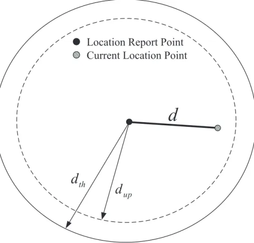
In contrast with the time-based location reporting scheme, the distance-based location reporting scheme [5] is definitely different approach. In this scheme, each mobile device tracks the distance d which it moved since last reporting a location message, and it sends a location message again whenever the dis-tance d exceeds a certain parameter dupcalled distance-based location report condition. However, because of the required location error tolerance from each location-based application server, we must also guarantee that each lo-cation calculation is within this tolerance value. The selected lolo-cation error tolerance determines the report threshold dth, which must not be exceeded by the difference of the two location reports. Figure 2.2 shows how the

distance-based location reporting scheme reports the current location. According to the observations, the distance-based location report condition dup dominates system performances, including the location error and the overall power con-sumption. For example, if a mobile device is with the smaller dup, it causes the overall power consumption to increase but decreases location errors be-cause of frequent location reports. Consequently, the application server will track the mobile device accurately, but the mobile device will drain the bat-tery capacity rapidly. In an existing discussion [5], there are some methods for optimizing value dup.

2.2

Dynamic Programming

In this section, we introduce a mathematical optimization method called “dy-namic programming” which will be used in our proposed approach for op-timal energy-efficient location update. For optimization problems, dynamic programming is a general mathematical optimization approach for efficiently solving multi-stage optimization problems, or optimal planning problems. It refers to simplifying a complicated problem by breaking it down into sim-pler subproblems in a recursive manner. In addition, dynamic programming is suitable when subproblems are not independent, which called overlapping subproblems. That is, when subproblems share subsubproblems. This means that dynamic programming can solve each subsubproblem just once and then save its answer in a table, thereby avoiding the work of recomputing the an-swer every time. This is a benefit of reducing the number of computations.

For developing procedures of dynamic programming, there are three steps, including (1) characterize the overall structure of an optimization problem, (2) define and compute the value of cost function (or reward function)

re-th

d

up

d

Location Report Point

Current Location Point

d

Source node Node 1 Node 2 Node 3 Node 4 Node 5 Node 6 Destination node 5 4 8 2 3 5 5 6 4 5 7 5 6

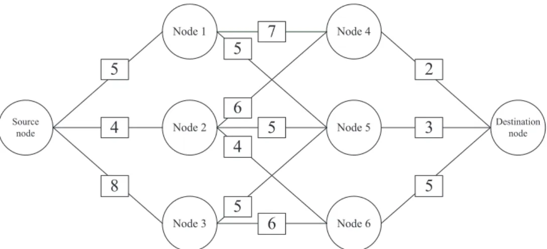
Figure 2.3: A topology for the shortest-path problem.

cursively at each stage, and (3) define and make an optimal solution from all computed information. The general example of a optimization problem with dynamic programming in the deterministic system is the shortest-path problem. Figure 2.3 illustrates a shortest-path topology for the minimum-distance problem.

In general, dynamic programming can solve the multi-stage optimization problem by using two recursive manners. They are shown as follows.

1. Forward Recursion: If the recursions proceed from the first stage to-ward the last stage, the recursive manner is called forto-ward recursion. The forward recursive relationship of the optimal-value function is shown as follows:

un+1(sn+1) = max

sn∈S{un(sn) + fn(sn, sn+1)} . (2.1) In (2.1), n represents the current stage and its range is from 0 to N (the number of stages). un(sn) is the optimal value of all prior decisions.

Note that we are in state snand the computations are usually initialized by setting u0(s0) = 0. fn(sn, sn+1) is the reward for a particular stage

n with the current state sn and the next state sn+1.

2. Backward Recursion: By symmetry, if the recursions proceed from the last stage toward the first stage, the approach is called backward recur-sion. The backward recursive relationship of the optimal-value function is shown as follows:

un(sn) = max

dn∈Dn{fn(dn, sn) + un+1(tn(dn, sn))} . (2.2) By contrast, in (2.2) un(sn) is the optimal value of all the subsequent decisions. Note that we are in state sn and the computations are usu-ally initialized by setting uN(sN) = 0. Furthermore, fn(dn, sn) is the reward for a particular stage n with decision dn and state sn. dn is a permissible decision that may be chosen from the set Dn, and tn(dn, sn) is a transition function which determines the new state at the next stage (i.e. sn+1= tn(dn, sn)).

In general, we can adopt one of these two approaches to solve problems. However, there is a primary difference in the ”by-products” resulted from these two approaches. In solving a problem by backward recursion, we will obtain by-products which are the optimal values from every state in every stage to the end. Whereas in solving a problem by forward recursion, the corresponding by-products would be the optimal values from the initial state in the first stage to every state in the remaining stages.

For example, in Fig. 2.3, we wish to find the shortest path from the source node to the destination node. The number next to the arcs are distances (or

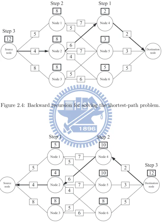
called costs). All corresponding costs are known in advance. A source node has also been added to illustrate that the dynamic-programming solution by using backward recursion finds the shortest path from the destination node to the source node. Essentially, it finds the shortest path from the destina-tion node to all nodes in the topology, thereby solving the minimum-distance problem for any source node. The calculation steps and results with back-ward recursion are shown in Fig. 2.4. The dynamic-programming solution by using forward recursion finds the shortest path from the source node to the destination node. The calculation steps and results with forward recursion are shown in Fig. 2.5. Although the shortest path will be the same for both methods, forward recursion will not solve the minimum-distance problem for any source node, since all source nodes are not the same. On the other hand, for the problems with uncertain planning horizons, forward recursion has an advantage over backward recursion. Therefore, when using dynamic pro-gramming, it is necessary to consider whether forward or backward recursion is the best suitable to the problem you want to solve.

Subsequently, in the real environment, dynamic programming can be used in the deterministic system or the stochastic system. However, in stochastic system the backward recursion is required because of the probabilistic nature of the markov decision process (MDP) [15, 16]. In contrast, if the system were deterministic, policies could be evaluated by either forward or backward recursion because expectations need not to be computed.

For our problem, we hope to solve the overall power consumption for lo-cation report in any system. We find the a proper optimization approach which is called dynamic programming that can satisfy the above require-ment. If we only know the transition probabilities, we have a stochastic dy-namic programming problem. Especially, the optimization problem with the

Source node Node 1 Node 2 Node 3 Node 4 Node 5 Node 6 Destination node 5 4 8 2 3 5 5 6 4 5 7 7 6 2 3 5 8 8 8 12 Step 1 Step 2 Step 3

Figure 2.4: Backward recursion for solving the shortest-path problem.

Source node Node 1 Node 2 Node 3 Node 4 Node 5 Node 6 Destination node 5 4 8 2 3 5 5 6 4 5 7 7 6 10 10 8 5 4 8 12 Step 1 Step 3 Step 2

stochastic dynamic programming can be called “markov decision processes (MDPs)” [15, 16]. The optimization problem with the deterministic dynamic programming was introduced in the previous section (e.g. the shortest-path problem). Here we are going to especially introduce the fundamental concept of markov decision processes and explain the details for finding the optimal solution.

2.2.1

Markov Decision Processes

The concept in markov decision processes is substantially applied in the op-timization problem with the stochastic dynamic programming. In fact, a markov decision process is also a discrete time stochastic process. A markov decision process model consists of five primary elements, including (1) stages

n, (2) states s, (3) actions a, (4) transition probabilities pr, and (5) returns

r (rewards or costs).

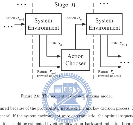
A markov decision process model is the sequential decision making model shown in Fig. 2.6. At each stage n, the action chooser observes the system state sn and selects an action an based on this system state. The system environment responds at the next stage by randomly changing to a new state sn+1, and giving the action chooser a corresponding return rn. The corresponding return rn is based on states sn, sn+1 and action an. Hence,

rn can be represented by rn(sn+1|sn, an). The transition probability that the system state changes to sn+1 as a new state is influenced by the chosen action

an. In particular, it is given by the state transition probability function

pr(sn+1|sn, an). Consequently, the next state sn+1 depends on the current state sn and the chosen action an.

For solving the optimization problem with stochastic dynamic program-ming (or called markov decision processes), the backward recursion is

re-1 n

r

r

Action

Chooser

System

Environment

System

Environment

s

a

a

s

Stage

n

Figure 2.6: The sequential decision making model.

quired because of the probabilistic nature of the markov decision process. In general, if the system environment were deterministic, the optimal sequence actions could be estimated by either forward or backward induction because expectations need not to be computed. However, all actions depend on fu-ture behavior, and only the history is known for forward recursion. Therefore, when using dynamic programming, it is necessary to consider if forward or backward recursion is suited to the optimization problem.

In order to illustrate how markov decision process model is applied in the stochastic dynamic programming, Fig. 2.7 shows the two-state system diagram with the current state sn = s(1). In this diagram, two actions have

been allowed in the first state s(1). If the action chooser selects action “1”

(an = 1, the solid line), then the transition from state s(1) to state s(1) will

Stage n

Stage

_{n +}

1

(1)

S

(2)

S

(1)

S

(2)

S

Figure 2.7: The two-state system diagram with the current state sn= s(1).

to state s(2) will be influenced by the probability pr(s(2)|s(1), 1). The returns

related to these transitions are r(s(1)|s(1), 1), r(s(2)|s(1), 1). If the second action “2” in state s(1)is chosen (an= 2, the dashed line), then pr(s(1)|s(1), 2), pr(s(2)|s(1), 2) and r(s(1)|s(1), 2), r(s(2)|s(1), 2) would be the relevant transition probabilities and returns, respectively. Using the same concepts, the relevant transition probabilities and returns in the second state s(2) can be defined.

The corresponding system diagram with the current state sn= s(2) is shown

in Fig. 2.8.

In order to find the optimal sequence actions, we define un(sn) as the total expected returns at n stage starting from state sn if an optimal policy is followed. If the returns are rewards, the definition of the total expected return through backward recursion is shown as follows.

Stage n

Stage

_{n +}

1

(1)

S

(2)

S

(1)

S

(2)

S

un(sn) = max an∈A{

∑ sn+1∈S

pr(sn+1|sn, an)· [r(sn+1|sn, an) + un+1(sn+1)]} , (2.3)

where n is from 0 to N (the number of stages) and

r(sn, an) = ∑ sn+1∈S

pr(sn+1|sn, an)· r(sn+1|sn, an) . (2.4)

We can use (2.4) to simplify (2.3), then get

un(sn) = max

an∈A{r(sn, an) + ∑ sn+1∈S

pr(sn+1|sn, an)· un+1(sn+1)} . (2.5)

The optimal control policy will be

a∗_n(sn)∈ arg max

an∈A {r(sn, an) + ∑ sn+1∈S

pr(sn+1|sn, an)· un+1(sn+1)} , (2.6)

where these policies can be represented by vector a∗ = (a∗₀, a∗₁, . . . , a∗_N−1). The utilization of the recursive equation (2.6) will inform the action chooser which action to use in each state sn at each stage n, and make overall system with the maximum expected future rewards at each stage of the process by using policy vector a∗. In Chapter 4, we will define all the elements for our problem based on the definitions of markov decision processes, and investigate how to optimally find the sequence actions with an objective of minimizing the power consumption for location updates by using stochastic dynamic programming (or called markov decision process) and backward recursion.

Chapter 3

System Models

3.1

System Architecture

We consider a system architecture which is based on the distance-based loca-tion reporting scheme. Each mobile device moves with the specific movement (e.g. fixed speed or random behavior). As it was mentioned in Chapter 2, the fundamental concept based on the distance-based location reporting scheme is that each mobile device essentially reports locations with a certain dis-tance. The system architecture consists of the following elements.

Location Error Tolerance dth

In general, each location-based application server must have the the required location error tolerance. The selected location error tolerance determines the location report threshold dth, which must not be exceeded by the difference of the two location reports. As a designer of location update scheme, we must also guarantee that each location calculation is within this tolerance value.

th

d

t

t

t

( )

d t

( )

d t

( )

d

_-

d t

( )

d

_-

d t

Location Report Point

Location Calculation Point

0

( )

th

d

_-

d t

Figure 3.1: The system architecture. Next Location Calculation Period

As it was mentioned in the introduction for location error tolerance, we must also guarantee that each location calculation is within the required location error tolerance dth from each location-based application server. We refer to the DBLR scheme [5] to decide the next location calculation period based on the current location in order to satisfy the above requirement.

decides the next location calculation period based on the current location. At every time point tj (the time point of the j-th location calculating a location since last reporting a location) for calculating a location, we can get the current location loc(tj) and calculate the distance d(tj) from the last reporting a location (i.e. d(tj) = |loc(tj)− loc(t0)|). Hence, we can know how far it is from the current location to the location report threshold (i.e.

dth- d(tj)). Subsequently, if we get the above parameters and the maximum moving speed vmaxof each device, we can decide the next location calculation period to guarantee that each location calculation is within the location error tolerance. Referring to [5], the formula of the next location calculation period

T(j) (the j-th location calculation period after last reporting a location) is shown as follows:

T(j)= dth− d(tj−1)

vmax

. (3.1)

Location Report Condition dup

At each mobile device, calculating a new location from the location sensor always requires an amount of time Tloc before the location is obtained. Due to the requirement for guaranteeing location error tolerance dth, the DBLR scheme [5] report condition must be at least

T(j)< Tloc . (3.2)

However, by using equation (3.1), the equation (3.2) can be simplified to

dth− d(tj−1)

vmax

< Tloc ,

Consequently, the location report condition dup for the distance-based loca-tion reporting scheme is

d(tj−1) > dup , where

dup= dth− vmax· Tloc . (3.4)

3.2

Hovering Around Border Effects

In the previous section, we guaranteed location error tolerance dth by us-ing equation (3.4). Its fundamental concept is that usus-ing the next proper location calculation period which is defined in (3.1) to guarantee that the corresponding distance d(tj) for each calculating location tj is within loca-tion error tolerance dth. However, the main drawback of (3.1) is that when the mobile device comes to the location report condition dup, the frequency of location calculation increases because the next location calculation pe-riod becomes shorter. Consequently, when the mobile device approaches to the location report condition, the power consumption may increase rapidly. We call this phenomenon the power consumption problem of hovering around

border. The phenomenon is also mentioned in [5]. This effect causes the

mobile device to drain the battery rapidly. In [5], a proposed method, called “early distance-based reporting” scheme, solves this problem by using some optimization solutions. Nevertheless, this approach can not accurately solve the problem in the stochastic system (or called prediction-based system). In the following chapters, we will introduce how our proposed approach solves the power consumption problem of hovering around border in both the de-terministic system and the stochastic system.

3.3

Performance Metrics

In this part, we define three primary performance metrics for three different location update schemes (TBLR, DBLR and EBLR). In our problem, we are concerned about the overall power consumption and location errors for location update schemes. Their definitions are shown as follows.

3.3.1

Average Power Consumption P = P

+ P

We are concerned to calculate the average power consumption as the over-all power consumption for different location update schemes. We use the average power consumption (3.5) rather than the definition in [5] because the observation concept in our proposed approach is the “stages” instead of the “time”. Therefore, the average power consumption in our definition is the average value of each immediate power consumption at each stage. The corresponding definition is shown as follows.

P , T he sum of power consumption

T he number of stages = N ∑ n=1 c(n) N , (3.5)

where Pc is the average power consumption of location calculation, and Pr is the average power consumption of location report. Furthermore, N is the number of stages, and c(n) is the cost function at n-th state transition. In other words, the average power consumption is the average value of each immediate cost function.

On the other hand, the computation power is the other design issue for mobile devices. However, in this thesis we do not consider the computation power of our algorithm. We assume that required energy for energy complex-ity [17] [18] of markov decision process in one-time execution is much smaller

than location updates.

3.3.2

Average Location Error L

Besides the power consumption, we consider the magnitude of location errors. The first consideration is the magnitude of the average location error. This performance metric represents the perspective of average value on location errors for different location update schemes. We observe all location errors within the specified observation stage N . Hence, the average location error can be calculated from all location errors. The corresponding definition is shown as follows.

Le,

T he sum of location errors T he number of location errors =

M ∑ i=1 Le(i) M , (3.6) where

Le(i) =|locat server(i)− locreal(i)| , (3.7) note that locat server(i) is the location at application server and locreal(i) is the real location of the mobile device. M is the number of location errors. Each location error is obtained by sampling both locat server(i) and locreal(i) every specific time (we use 0.1 seconds).

3.3.3

Maximum Location Error L

The other consideration is the magnitude of the maximum location error. This performance metric represents the perspective of maximum value on location errors for different location update schemes. It is also an index on location errors for the worst value. Based on these samples of location error,

we can obtain the magnitude of the maximum location error for each trial. The corresponding definition is shown as follows.

Le max= max

i=1,2,...,M{Le(i)} . (3.8)

Based on the above definitions for performance metrics, we will apply them in the following chapters and investigate the corresponding results by using simulations.

Chapter 4

Proposed Energy-Efficient

Location Update Mechanism

In this chapter, we introduce a power-aware location update scheme, called energy-based location reporting (EBLR), which applies dynamic program-ming to the traditional distance-based location reporting technique to deter-mine the optimal location update scheme with an objective of minimizing power consumption in mobile computing. Through dynamic programming, the EBLR can energy-efficiently change the frequency of location calcula-tion and locacalcula-tion report at every decision time point (stage) in any system. The corresponding contents of our proposed approach are presented in the following sections.

4.1

Assumptions

For stochastic dynamic programming, the deterministic dynamic program-ming can be said by the specific case of markov decision processes. Con-sequently, in this thesis, we only introduce general case (i.e. the stochastic

case) for our proposed approach. In the stochastic environment, location-based applications only know the statistics of the system. The statistics of the system may be the probability distributions of the terminal moving directions or moving speeds. By using the probability distributions of statis-tics, the corresponding state transition probabilities may be obtained. Our stochastic system is based on the above conditions. We assume that the location-based application can obtain the probability distributions of statis-tics. Furthermore, we also assume that the cost function and the transition probability are stationary (In a word, their value or distribution are time-invariant). A simple stochastic system is described in Fig. 4.1. The terminal device moves with the fixed speed v but with random forward angle θ.

In the next section, we will use a simple example to illustrate the following definitions for optimal energy-efficient location update scheme.

4.2

Definitions

We define the state presentations, actions, transition probabilities, cost func-tions, and the principle of optimality for our problem.

4.2.1

System States

In the DBLR scheme, we know that the next location calculation period is related to the distance d(tj) (d(tj) = |loc(tj)− loc(t0)|). Hence, we use the distance d(tj) to represent each system state in the EBLR scheme because our proposed approach, the EBLR scheme, refers to the next location cal-culation period in the DBLR scheme. However, it is difficult to definitely separate discrete states because of the continuity of distance. Therefore, we use the multiples of the shortest location calculation period Tloc(or called the

next

v T

×

q

p

-2

p

0

d

Last Location Report Point Current Location Calculation Point Next Location Calculation Point 1 2 _{2 2}

[(

cos )

(

sin ) ]

d

¢ =

d

+

v T

×

×

q

+

v T

×

×

q

d ¢

Table 4.1: The System Parameters for Illustration.

Parameter Value

Required Time for

Calculating a Location, Tloc 0.5 seconds

Maximum Speed, vmax 10 m/s

Report Threshold, dth 100 meters

required time of calculating a location) as the discrete states. It is beneficial that the continuous distance can be definitely separated into discrete states. Our approach is to use this concept to represent each state.

We use a simple example to illustrate how we define our system states. The system parameters are shown in Table 4.1 for illustration. For example, in Fig. 4.2, the range of distance is divided up into twenty states (s(1), s(2),. . ., s(19) and s(20)) based on the system parameters in Table 4.1. In addition,

each state has an individual range of distance. For any distance in the same state, all the next location calculation periods will be the same by using the minimum location calculation period (e.g. the minimum location calculation period is 19·Tlocin the state s(2), then Tnext = 19·Tlocfor any distance in the state s(2)). The corresponding next location calculation period Tnext which can be obtained by using equation (3.1). They are shown in Table 4.2.

From the above calculations, we can also define the state transitions in this stochastic system example. The state transition diagrams are shown in Fig. 4.3.

In Fig. 4.3, when the decision maker chooses action a at the current stage n, the corresponding immediate cost function (4.8) is c(sn, a) and the corresponding state transition probability is psnsn+1(a). In the following sec-tion, we will define the corresponding state transition probability for optimal

(2) s (20) s (19) s Last Updating Location 0 d = d =5 d =90 d =95 (1) s

2

×

T

įįį

(2)

s

s

1

a =

0

a =

( ,

1)

c s

a =

( ,

0)

c s

_{a =}

1

p

₌

p

Stage n

Stage

_{n +}

1

s

p

s

p

p

n

S

Table 4.2: All States.

The Range of Next Location State Distance (m) Calculation Period

s d Tnext(s) s(1) d = 0 20· Tloc= 10 s s(2) d∈ (0, 5] 19· Tloc= 9.5 s .. . ... ... s(19) d∈ (80, 85] 2· Tloc= 1 s s₍₂₀₎ d∈ (90, 95] Tloc= 0.5 s

energy-efficient location update.

4.2.2

Action Representations

In our scenario, we only have two actions to choose at each decision time point (stage). One is the action which represents that the mobile device will only calculate the current location at the next location calculation time point (stage), denoted by symbol “0”. The other is the action which represents that the mobile device will both calculate and report the current location at the next location calculation time point (stage), denoted by symbol “1”.

4.2.3

Transition Probabilities

For the stochastic system, p(j|i, a) denotes the probability that the system is in state j at the next stage when the decision maker chooses action a in state i at the current stage. Here, we define the corresponding transition probabilities p(j|i, a) for the stochastic system shown in Fig. 4.1. They are shown as follows:

location) p(j|i, a = 1) =    1 , j = s(1) and i∈ S 0 , otherwise . (4.1)

2. When the chosen action a = 0 (only calculating the current location)

p(j|i, a = 0) = p(Blower(j) < d ′

≤ Bupper(j)) , (4.2)

where

d′ =√[d + v· Tnext(i)· Cosθ]2+ [v· Tnext(i)· Sinθ]2 , (4.3) and

d∼ U(Blower(i), Bupper(i)) , θ ∼ U(−π/2, π/2) . (4.4)

Tnext(s) is the next location calculation period when the state is s. Blower(s) is the lower boundary of distance range when the state is s. By contrast,

Bupper(s) is the upper boundary of distance range when the state is s. For example, in Table 4.2, Tnext(s(20)) is 0.5 (s), Blower(s(20)) is 90 (m), and Bupper(s(20)) is 95 (m).

In equation (4.1), we define the transition probabilities for action a = 1. Note that as long as the chosen action a is “1” for any state snat the current stage n, the state sn+1 at the next stage n + 1 will always be the first state

s(1) which represents the point of reporting the current location (i.e. d = 0).

Otherwise, other transition probabilities are zero.

On the other hand, in equation (4.2), we define the transition probabilities for action a = 0. All transition probabilities can be obtained by using (4.2) (4.3) (4.4) and integral operations. Figure 4.4 illustrates how the transition probability can be obtained. For example, if we are going to obtain the

transition probability p(j = s(4)|i = s(2), a = 0) based on all state definitions

in Table 4.2, then the transition probability can be simplified to

p(j = s(4)|i = s(2), a = 0) = p(Blower(s(4)) < d ′ ≤ Bupper(s(4))) = p(10 < d′ ≤ 15) , (4.5) where d′ = √

[d + v· Tnext(s(2))· Cosθ]2+ [v· Tnext(s(2))· Sinθ]2 , (4.6)

and

d∼ U(Blower(s(2)), Bupper(s(2))) , θ ∼ U(−π/2, π/2) . (4.7)

By using (4.5) (4.6) (4.7) and integral operations, we can obtain the corresponding transition probability.

4.2.4

Cost Functions

Because the main objective is to minimize the power consumption of calcu-lating and reporting locations at the mobile device, we define that the cost function is the power consumption between each decision time point (stage). As we know that the power consumption between each decision time point (stage) is related to each location calculation period and action. The formula is shown as follows:

c(i, a), Immediate energy consumption

N ext location calculation period = ϵ(a)

τ (i) . (4.8)

c(i, a) is the immediate cost function when the decision maker chooses

action a in state i at the current stage. Furthermore, ϵ(a) is the energy function of action a and the next location calculation period τ (i) is the

next v T× q 2 p -2 p 0

d

Last Reporting Location Point Current Location Calculation Point Next Location Calculation Point

d ¢

s

[( next cos ) ( next sin ) ]

d¢ = d+v T× × q + v T× × q ~ [ _lower( ), _{n upper}( )]_n d U B s B s ~ [ , ] 2 2 U p p q

-Figure 4.4: An illustrative example of calculating the transition probability. function of state i. Based on the definition for the action, ϵ(a) is defined as follows. ϵ(a) =    Ec , a = 0 Ec+ Er , a = 1 . (4.9)

Subsequently, τ (i) is defined as follows.

τ (i) = Tnext(i), i∈ S , (4.10)

where S is a set for system states. For example, if system states are based on Table 4.2, the corresponding τ (i) is defined as

τ (i) = Tnext(i), i∈ s(1), s(2), . . . , s(19), s(20) . (4.11)

each stage as the immediate cost function. That is why we call our approach the energy-based location reporting scheme.

4.3

Optimal Energy-Efficient Location Update

Algorithm

In this section, we are going to introduce an optimal energy-efficient location update algorithm. The principle of optimality with DP and the procedure of power consumption minimization are shown as follows.

4.3.1

Principle of Optimality

Recall that we consider all system elements (states, actions, transition prob-abilities and cost functions), the principle of optimality for the stochastic location update in our proposed approach, the energy-based location report-ing scheme, can be identified by usreport-ing the above system elements.

1. Recursion Manner (Bellman’s Equation): Because of the stochas-tic system, here we can use the backward recursion manner to find the optimal value function un(sn), and the computations are initialized by setting uN(sN) = 0. Furthermore, anis a permissible decision that may be chosen from the set A=0,1, and n = 0, . . . , N − 1.

un(sn) = min an∈A{c(sn, an) + ∑ sn+1∈S pr(sn+1|sn, an)· un+1(sn+1)} . (4.12) 2. Optimal Policy: Any element of Markov policy vector a∗ satisfies the

a∗_n(sn)∈ arg min an∈A {c(s n, an) + ∑ sn+1∈S pr(sn+1|sn, an)· un+1(sn+1)} . (4.13)

This optimal control policy is called the stochastic Markov policy. Through backward recursion, we can find the optimal solution for scheduling the sequence actions (i.e. vector a∗) of each mobile device in the stochastic system.

4.3.2

Procedures of Power Consumption Minimization

In this section, we present the procedure of power consumption minimization by using the optimal energy-efficient location update algorithm with three steps. The algorithm solves optimality equation (4.12) subject to boundary condition uN(sN) = c(sN). The steps for the optimal energy-efficient location update algorithm are shown as follows.

• Step 1 : Set n = N and

uN(sN) = c(sN), for each sN ∈ S , where c(sN) is usually set to zero.

• Step 2 : Substitute n − 1 for n and then compute un(sn) for each

sn ∈ S by un(sn) = min an∈A{c(sn, an) + ∑ sn+1∈S pr(sn+1|sn, an)· un+1(sn+1)} .

Set a∗_n(sn)∈ arg min an∈A {c(s n, an) + ∑ sn+1∈S pr(sn+1|sn, an)· un+1(sn+1)} .

• Step 3 : If n = 0, stop. Otherwise return to step 2.

Figure 4.5 shows the flow chart of optimal energy-efficient location up-date algorithm. The minimum power consumption can be achieve in this algorithm.

In the following chapter, we will use this algorithm and compare our pro-posed energy-based location reporting method with other approaches (DBLR and TBLR) in depth by using simulations.

Initial condition

Set n=N and boundary condition:

Substitute

n

-

1 to

n

å

å

Find the optimal solution

if

n <

1

Start

End

No

Yes

Figure 4.5: The flow chart of optimal energy-efficient location update algo-rithm.

Chapter 5

Numerical Results

In this chapter, we show numerical results to reveal the importance of the two key impact factors on performance metrics for different location update schemes in the stochastic system. The impact factors consist of (1) the energy ratio Er/Ec, and (2) the terminal moving speed v. Furthermore, we verify that with our proposed approach the effects of the above factors on the overall system power consumption can be decreased by implementing optimal energy-efficient location update algorithm.

5.1

Simulation Setup

For the stochastic system, we simulate the terminal moving environment with the given speed v and the random forward angle θ. The random forward an-gle θ is a random variable with the uniform distribution from −pi/2 to pi/2. Moreover, the terminal moves with the fixed moving speed but goes for-wards with the random angle. The terminal moving environment is shown in Fig. 4.1. We consider three location update schemes, including (1) the time-based location reporting scheme (TBLR), (2) the distance-time-based location

Table 5.1: The System Parameters.

Parameter Value

Required Time for

Calculating a Location, Tloc 0.5 seconds

Maximum Speed, vmax 10 m/s

Speed, v Fixed (1 m/s to 10 m/s) Moving Direction Random angle θ ∼ U(−π/2, π/2) Report Threshold, dth 100 meters

Report Condition, dup 95 meters

Energy for

Calculating a Location, Ec 75 mJoules

reporting scheme (DBLR), and our proposed approach (3) the energy-based location reporting scheme (EBLR). Furthermore, we use the system param-eters in Table 5.1 except that the energy Er of reporting locations and the terminal moving speed v are set in different values for different conditions. The trial times for simulation are set to be bigger than 100 times. On the other hand, the number of stages N is set to be bigger than 100.

5.2

Effects of Energy Ratio on Power

Con-sumption for Various Location Update Schemes

with Different Terminal Moving Speeds

Firstly, in the stochastic system we investigate the effects of the energy ra-tio Er/Ec on power consumption for various location update schemes with different terminal moving speeds v. In general, different energy ratios satisfy different amounts of reporting information. For example, if the mobile device

sends the location data which is like the format [+24.789462,+121.000113], it needs to at least consume about 15 mJoules energy for transmitting 182 bits location data [19]. Hence, different energy ratios represent that they are applied in different location-based applications. In order to evaluate the performance on power consumption for various energy ratios and different terminal moving speeds, we consider that the value range of the energy ratio is 2−10 to 210 and the value range of the terminal moving speed is 1 (m/s) to 10 (m/s).

Figure 5.1 shows how the terminal moving speed and the energy ratio affect the overall system power consumption in the stochastic system. We use the general energy ratio value (i.e. The line for Er = 15 mJoules) to ob-serve the effect on each curve. We obob-serve that in each subfigure the overall system power consumption increases with the energy ratio Er/Ecfor location updates when the energy ratio is bigger than the general energy ratio value. Moreover, each subfigure represents the effect of the energy ratio on power consumption for various location update schemes with a certain terminal moving speed. Figure 5.1 also shows that the energy Er of reporting loca-tion significantly affects the power consumploca-tion for various localoca-tion update schemes. As the energy ratio increases, the power consumption increases due to the increasing energy of location report.

Nevertheless, the energy ratio Er/Ec effects location update schemes dif-ferently on power consumption with various terminal moving speeds. In Fig. 5.1(a), the DBLR scheme consumes less power than the TBLR scheme does when the energy of location report increases. It is because that the frequency of location report with the DBLR scheme decreases when the ter-minal moving speed decreases. As the terter-minal moving speed increases, in Figs. 5.1(b) and 5.1(c), the DBLR scheme consumes more power than other

−105 −5 0 5 10 10 15 20 25 30 35 40 45 50 log 2 Er/Ec Power (dBm) TBLR DBLR EBLR Er=15 mJoules

Decrease Max 30% Power

(a) The terminal moving speed v = 1.

schemes because the frequency of both reporting and calculating location increases. However, as the terminal moving speed achieves maximum speed

vmax, in Fig. 5.1(d), all location update schemes use the same period of re-porting and calculating location.

Due to the use of stochastic dynamic programming (4.12) (4.13), in the case of any terminal moving speeds the EBLR scheme can dynamically and optimally select actions which consume less power by using the statistics of system (i.e. state transition probabilities). That is the reason why the EBLR scheme which uses the stochastic dynamic programming is always the best solution when the energy ratio varies for location updates. Moreover, in this simulation we prove that in EBLR the maximum saving power can

−105 −5 0 5 10 10 15 20 25 30 35 40 45 50 log 2 Er/Ec Power (dBm) TBLR DBLR EBLR E r=15 mJoules

Decrease Max 14% Power

−105 −5 0 5 10 10 15 20 25 30 35 40 45 50 log 2 Er/Ec Power (dBm) TBLR DBLR EBLR E r=15 mJoules Decrease Max 0.6% Power

−105 −5 0 5 10 10 15 20 25 30 35 40 45 50 log 2 Er/Ec Power (dBm) TBLR DBLR EBLR Er=15 mJoules Decrease Max 0% Power

(d) The terminal moving speed v = 10.

Figure 5.1: Effects of the energy ratio on the overall system power con-sumption for various location update schemes with different terminal moving speeds.

be about 30 percent which is compared to the other better scheme. We also observe that the EBLR is suitable for solving the power consumption problem of hovering around border (i.e. the terminal moving speed is lower). In other words, the EBLR does not have obvious advantages when the terminal moving speed is higher (the maximum saving power is close to 0 percent).

5.3

Effects of Terminal Moving Speeds on

Lo-cation Errors for Various LoLo-cation

Up-date Schemes with Different Energy

Ra-tios

In this part, we are going to evaluate other performance metrics, location errors, including (1) average location errors and (2) maximum location er-rors for location updates. Likewise, we also consider three different location update schemes, including TBLR, DBLR, and EBLR, then investigate the effects of the terminal moving speeds v on power consumption for various location update schemes with different energy ratio Er/Ec. Moreover, as it was mentioned in Chapter 1, we use the minimum city block distance (i.e. it is 80 meters) as the maximum tolerable location error for our application, location-based social network. On the other hand, we straightforwardly use a half of the minimum city block distance (i.e. it is 40 meters) as the average tolerable location error.

Average Location Errors

Figure 5.2 illustrates the average location errors related to terminal moving speeds with different energy ratios for location updates. The figure shows

some phenomena for various location update schemes. For the DBLR scheme, the average location errors have less variation because the location report condition is based on terminal moving distance d. Even though the terminal moving speed increases, it still do not report a location when the terminal moving distance d does not exceed the location report condition dup. Conse-quently, the average location errors with the DBLR scheme are always larger than other schemes. We observe that in the DBLR the average location er-rors are larger than the average tolerable location error (40 meters) for any case. In contrast, the TBLR scheme always reports locations with a fixed period. This effect leads to a result that the average location errors increase when the terminal moving speed increases.

Nevertheless, the EBLR scheme reports locations by using power-aware decision (4.12) (4.13) based on the stochastic dynamic programming. The power-aware approach leads to a result that the optimal decision must se-lect the result of potentially making the longer period for calculating and reporting locations when the terminal moving speed increases. This trends to choose the action “1” which represents that the mobile device will both calculate and report the current location. It implied that the location report condition with the EBLR scheme is similar to the TBLR scheme whenever the terminal moving speed increases. That is the reason why the average location errors with the EBLR scheme are always better than the DBLR scheme but usually worse than the TBLR scheme does in trial samples.

On the other hand, in Figs. 5.2(b) and 5.2(c), for location updates we also observe that with the lower terminal moving speeds, the EBLR scheme has larger average location errors when the energy ratio increases. The reason is that the EBLR scheme trend to optimally choose the sequence actions in order to minimize the expectation of overall system power consumption, but

1 2 3 4 5 6 7 8 9 0 5 10 15 20 25 30 35 40 45 50 Speed (m/s)

Average Location Error (m)

TBLR DBLR EBLR

tolerable average location error

0 meter

1 2 3 4 5 6 7 8 9 0 5 10 15 20 25 30 35 40 45 50 Speed (m/s)

Average Location Error (m)

TBLR DBLR EBLR tolerable average location error

12 meters

1 2 3 4 5 6 7 8 9 0 5 10 15 20 25 30 35 40 45 50 Speed (m/s)

Average Location Error (m)

TBLR DBLR EBLR tolerable average location error

31 meters

(c) log2Er/Ec= 5.

Figure 5.2: Effects of the terminal moving speed on average location errors for various location update schemes with different energy ratios.

sacrifices the better performance on the average location errors. However, in the EBLR we also observe that even through the average location errors will increase when the terminal moving speed is lower, they are still in satisfied level (i.e. they are all smaller than the average tolerable location error, 40 meters) for providing our location-based services. This proves that EBLR can provide a better balance between power consumption and location error than other schemes.

Maximum Location Errors

Figure 5.3 illustrates the maximum location errors related to terminal moving speeds with different energy ratios. For the effects of the terminal moving speed, the simulation results in each location update scheme on the maximum location errors are similar to the average location errors. Likewise, for the DBLR scheme, the maximum location errors have less variation because the location report condition is based on terminal moving distance d. Even though the terminal moving speed increases, it still do not report a location when the terminal moving distance d does not exceed the location report condition dup. Consequently, the maximum location errors with the DBLR scheme are always larger than other schemes. We observe that in the DBLR the maximum location errors are larger than the maximum tolerable location error (80 meters) for any case. In contrast, the TBLR scheme always reports locations with a fixed period. This effect leads to a result that the maximum location errors increase when the terminal moving speed increases.

Nevertheless, for the same reason, the EBLR scheme reports locations by using power-aware decision and distance-based location reporting scheme. The power-aware approach leads to a result that the optimal decision must select the longer period for calculating and reporting locations when the