行政院國家科學委員會專題研究計畫 成果報告
描點相關時多階製程管制方法之研究(2/2)
計畫類別: 個別型計畫 計畫編號: NSC91-2118-M-004-008- 執行期間: 91 年 08 月 01 日至 92 年 07 月 31 日 執行單位: 國立政治大學統計學系 計畫主持人: 楊素芬 計畫參與人員: 何漢葳蘇惠君何志傑劉家銘蔡淑芳 報告類型: 完整報告 處理方式: 本計畫涉及專利或其他智慧財產權,2 年後可公開查詢中 華 民 國 92 年 10 月 27 日
行政院國家科學委員會補助專題研究計畫
□ * 成 果 報 告
□期中進度報告
描點相關時多階製程管制之研究
計畫類別:□* 個別型計畫 □ 整合型計畫
計畫編號:NSC 91-2118-M -004-008-
執行期間: 90 年 8 月 1 日至 92 年 7 月 31 日
計畫主持人:楊素芬教授
共同主持人:
計畫參與人員: 何漢葳、蘇惠君、何志傑、劉家銘、蔡淑芳
成果報告類型(依經費核定清單規定繳交):□精簡報告 *□完整報告
本成果報告包括以下應繳交之附件:
□赴國外出差或研習心得報告一份
□赴大陸地區出差或研習心得報告一份
□出席國際學術會議心得報告及發表之論文各一份
□國際合作研究計畫國外研究報告書一份
處理方式:除產學合作研究計畫、提升產業技術及人才培育研究計畫、列
管計畫及下列情形者外,得立即公開查詢
□涉及專利或其他智慧財產權,□一年□*二年後可公開查詢
執行單位:國立政治大學統計系
中 華 民 國 92 年 10 月 25 日
STATISTICAL PROCESS CONTROL FOR THE AUTOCORRELATED OBSERVATIONS UNDER TWO SUB-PROCESSES
Su-Fen Yang Department of Statistics
National Chengchi University Taipei, 116, Taiwan
ABSTRACT
The observations from the process output are always assumed independent when using a control chart to monitor a process. However, for many processes the process observations are autocorrelated. This autocorrelation can have a significant effect on the performance of the control chart. This paper considers the problem of monitoring the mean of a quality characteristic X on the first sub-process and the mean of a quality characteristic Y on the second sub-process, in which the observations X can be modeled as an AR(1) model and observations Y can be modeled as an transfer function of X since the state of the second sub-process is dependent on the state of the first sub-process. To effectively distinguish and maintain the state of the two dependent sub-processes, the Shewhart control chart of residual and the cause-selecting control chart are proposed. The proposed control charts’ performance is measured by the rate of true alarm or false alarm. From numerical analysis, it shows that the performance of the proposed control charts is much better than the Hotelling T control chart and the individual X and Y charts. 2
Key Words: Autocorrelated observations,control charts, process variation, residuals.
1. INTRODUCTION
Control charts are first proposed by Shewhart (1931), and become effective tools for improving the process quality and productivity.
different times are independent random variables. However, the independence assumption is often violated for processes in chemical and pharmaceutical industries. Observations from these processes are always autocorrelated. When the control charts developed under the independence assumption, the autocorrelated process results in decreasing the in-control average run length (ARL). For effective monitoring the autocorrelated processes, one popular developed approach is to constructing control charts using the residuals from the time series model to the process data (see Abraham and Kartha (1979), Alwan (1991), Alwan and Roberts(1988), Berthouex, Dooley, Kapoor, Dessouky and Delves (1986), Ermer (1980), Harris and Ross (1991), Montgomery (1996), Montgomery and Mastrangelo (1991), and Wardell, Moskowitz, and Plante (1992, 1994)). The properties of the proposed residual charts and their performance are investigated by Harris and Ross (1991), Longnecker and Ryan (1992),Yashchin (1993),Kramer and Schmid (1997), Schmid (1995),Lin and Adams (1996), Schmid (1997a), Padgett, Thombs and Padgett (1992), Runger, Willemain and Prabhu (1995), Vander Weil (1996), Timmer, Pignatiello and Longnecker (1998), Schmid (1997b) ,Zhang (1998), Schmid and Schone (1997), Alwan and Roberts (1988) and Lu and Reynolds (1999).
Much of the paper on the performance of control charts based on residuals has focused on the Shewhart control chart of residuals.
Today, many industrial products are produced by several dependent processes not just one process. Consequently, it is not appropriate to monitor these processes with a control chart for each individual process; what is needed is an appropriate method for controlling the processes.
Zhang(1984) proposes the simple cause-selecting chart to monitor the second process of the two dependent processes. Wade and Woodall (1993) review the basic principles of the cause-selecting chart for two dependent processes and suggest a modification to the use of simple cause-selecting chart. They also examine the relationship between the simple cause-selecting chart and the multivariate T2 control chart. In their opinion, the simple cause-selecting control chart has some advantages over the T2 control chart. However, the statistical process control approach to effectively distinguish and monitor the dependent sub-processes states for autocorrelated observations has not been addressed. In this paper, Shewhart chart of residuals and cause-selecting control chart are developed to monitor the large mean shift of the first process and the large mean shift of the second process, respectively. The performance of the proposed control charts for monitoring the two sub-processes is measured by the probability of alarms. Finally, a numerical example illustrates the application of the proposed control charts and its performance.
2. AUTOCORRELATED OBSERVATIONS FOR TWO SUB-PROCESSES
In this paper, we consider two dependent sub-processes, which may have two types of failure mechanisms. One type of the failure mechanisms occurs only in the first process and causes the mean shift of the quality variable (X), while the other type occurs only in the last process and causes the mean shift of the quality variable (Y). Two types statistical control charts will be derived to effectively distinguish and monitor the dependent sub-processes states for autocorrelated observations. Before describing how to derive the statistical control charts, the assumptions of the production processes behavior are given as follows.
2.1 Assumptions and Notation
Assumptions
(1) The production has two dependent processes. The first process is called the sub-process 1 and the second process is called the sub-process 2. The sub-process 1 and the sub-process 2 are dependent. So the quality variable X produced by the sub-process 1 will affect the quality variable Y produced by the sub-process 2. A pair of observations (xt,yt) are sampled from the end of the sub-process 2 every h time unit of sampling interval,t =1,2,3,...
(2) For autocorrelated observationsxtat sub-process 1, it is assumed that quality variable Xtcan be
written as an AR(1) model at time t with process meanξX, that is Xt =(1−φ)ξX +φXt−1+at ,t=1,2,...., (1)
where φ is the AR parameter satisfying |φ|<1. The at’s are assumed to be independent normal random variables with mean 0 and variance 2
a
σ .
Since X affects Y , the model relating the two variables can be written as a transfer function,
that is ,.... 2 , 1 , 1 1 0 + + = + =C V X V X − N t Yt Y t t t , (2)
whereCY is a constant and where Nt’s are assumed to be independent normal random variables
with mean 0 and variance 2
N
σ .
(3) When one failure mechanism occurs only in the sub-process 1, it will shift the mean of X.
This will also cause the mean of Y shifts. When the other failure mechanism occurs only in
(4) The time to sampling and charting one item is very small and negligible.
3. THE TIME SERIES MODEL FOR AUTOCORRELATED PROCESS
Time series model, especially AR(1) model, has been widely used to model many types of processes.
When the sub-process 1 is in control the minimum mean square error forecast (Box, Jenkins, and
Reinsel (1994)) made at time t−1 for time t is
1 ^ 0 ^ ^ ) 1 ( − + − = X t t X X φ ξ φ (3) The residual at time t is
^
t t Xt X X
e = − (4)
Suppose that a failure mechanism would cause a step change from ξX0to ξX1in the process mean
between time t=τ −1and τ . The expectations of the residual for various times are
,.... 2 , 1 , ) ( , , 2 1 0 ) ( 0 X1 1 0 X1 = + = − = − − − = = l l t t ,... , τ τ t e E X l X Xt τ ξ ξ φ τ ξ ξ (5)
The residuals are uncorrelated and normally distributed with variance 2
a
σ . We may find that the expectation of a residual after the shift occurs is a decreasing function of the time after the shift.
Hence, the probability of an alarm by a control chart of residuals in the sub-process 1 is the highest
for the sample immediately after the shift, and this probability continually decreases over time as
the forecast adapts to the shift.
In sub-process 2, a transfer function is used to express the relationship between quality variables Y
and X. The estimate for equation (2) is
The residual at time t is ^ t t Yt Y Y e = − (7)
Suppose that another failure mechanism would cause a step change from ξY0to ξY1in the process
mean between time t=τ'−1and τ'. The expectations of the residual for various times are
,.... 2 , 1 , 0 , , 2 1 0 ) ( ' ' 0 Y1 ' ' = + = = − − − = = l l t t ,... , t e E Y Yt τ τ ξ ξ τ τ (8)
The residuals are uncorrelated and normally distributed with variance 2
N
σ . Note that the shift of process mean only appears at time τ'after the failure mechanism occurs between time τ' −1and
'
τ .
4. CONTROL CHARTS CONSTRUCTION
A general form of control charts is represented as follows.
µ ±W kσW, (9)
where µW and σW are the mean and standard deviation of a control statistic, say Wt, when the
process is in control. The constant,k, is chosen to give a specified in control false alarm
probability. The k is frequently taken to be 3 to give an false alarm probability 0.0027 for a
Shewhart type control chart.
To monitor the sub-process 1, the Shewhart control chart of residuals plots the control statistic eXt,
,.... 2 , 1
=
t . For this control statistic, the control limits in equation (9) are
±3σa (10)
of quality variable Y, since quality variable Y is affected by quality variable X. The proposed
approach is to monitor the specific quality in the sub-process 2 by adjusting the effect of Y from X;
that is the specific quality is presented by the cause-selecting values (eYt =Yt −Y^t). When the
specific quality is in control, the cause-selecting control chart is constructed by the in-control
distribution of cause-selecting values.
For sub-process 2, the cause-selecting control chart plots the control statistic eYt, t=1,2,.... For this
control statistic, the control limits in equation (9) are
±3σN (11)
Consequently, the Shewhart control chart and cause-selecting control chart are derived to effectively
distinguish and monitor the process states of sub-process 1 and sub-process 2.
The variance of the control statistic eXtis usually unknown. The average moving range divided by
coefficient d2 is always taken as its estimate, that is
2 ^ d MRX a = σ , where 1 1 1 ) 1 ( − =
∑
− = − n MR MR n t t X X , andwhere MRX(t−1)=|eXt−eX(t−1)|,t=2,3,...n. Similar to the variance of the control statisticeYt, the estimate
of σN is 2 ^ d MRY N = σ , where 1 1 1 ) 1 ( − =
∑
− = − n MR MR n t t YY , and where MRY(t−1)=|eYt−eY(t−1)|,t=2,3,...n.. Thus the
control limits of Shewart control chart and cause-selecting control chart in equations (10) and (11)
can be expressed as 2 3 d MRX ± , (12) and 2 3 d MRY ± , (13)
respectively. Note that the value of d2is dependent on the sample size n(=2).
5. MEASUREMENT OF THE PERFORMANCE OF CONTROL CHARTS
The performance of a control chart can be measured by the probability of alarm. The probability of
false alarm is the rate of false alarm occurred on the control chart before a failure mechanism occurs
in the process, and the probability of true alarm is the rate of true alarm occurred on the control
chart after the failure mechanism occurs in the process and before it is removed. When the process
is out of control it is desirable to have a high rate of true alarm so that the change of process mean
will be detected quickly, and when the process is in control it is desirable to have a low rate of false
alarm. The probability of alarm for the developed two control charts will be calculated when both
the sub-processes are in control and when either one of or both the sub-processes means shift.
5.1 Calculating the Probability of Alarm for the Two Proposed Control Charts
The probability of false alarm for the Shewhart chart of residuals is 370.4, and same to the
cause-selecting chart. To monitor the two dependent sub-processes, two developed charts are used
simultaneously. Hence the probability of at least one false alarm for the two charts is 0.0054, that
is 1-0.9973x0.9973. To calculate the probability of true alarm for the two charts, we have to
compute the power of the Shewhart chart of residuals and cause-selecting chart, respectively. Let
the power of the Shewhart chart at time t isPs , and the power of the cause-selecting chart at time t t
(14) ,.... 2 , 1 , 0 , ), ) ( 3 ( 2 )) ( | 3 3 Pr( 2 1 1 0 0 1 1 2 2 = + = − − − Φ = − − < > = l l t MR d d MR e or d MR e Ps X X X l S X X l X Xt X Xt t τ ξ ξ φ ξ ξ φ , ' 0 1 2 0 1 2 2 ), ) ( 3 ( 2 )) ( | 3 3 Pr( > <− ξ −ξ = Φ − − ξ −ξ =τ = t MR d d MR e or d MR e Pc Y Y Y C Y Y Y Yt Y Yt t . (15)
where ΦSand ΦC are the cumulative standard normal probabilities, respectively.
Note that the power of the Shewhart chart of residuals decreasing over time, but not for the
cause-selecting chart. Hence the power for the two charts will be decreasing over time, once the
sub-process 1 is out of control.
There are four situations for the out-of-control process. The four situations and power of the two
charts are described as follows.
(1) The sub-process 1 is out of control but the sub-process 2 is in control. The power (Psc ) of the t
two charts is
Psct =1−(1−Pst)•(0.9973), t =
τ
+l, l=1,2,3,....(2) The sub-process 1 is in control but the sub-process 2 is out of control. The power (Psc ) of the t
two charts is
Psc =1−(0.9973)•(1−Pc ), t=τ'.
t t
(3) The sub-process 1 is out of control after timeτ −1, and the sub-process 2 is out of control after timeτ' −1, where τ <τ'. The power (
t
Psc ) of the two charts is
.... 3 , 2 , 1 , ), 9973 . 0 ( ) 1 ( 1 , ), 1 ( ) 1 ( 1 ), 9973 0 ( ) 1 ( 1 ' ' ' = < + • − − = − • − − < ≤ • − − = l t l Ps t Pc Ps t . Ps Psc t t t t t
τ
τ
τ
τ
time
τ
' −1, whereτ
" >τ
'. The power (t
Psc ) of the two charts is
. ) 9973 . 0 ( ) 1 ( 1 , ) 1 ( 9973 . 0 1 " '
τ
τ
≥ • − − = − • − = t Ps t Pc Psc t t t6. A Numerical Example and Some Comparison Results
A quality engineer found that there is a large variability for the thickness of the thin golden
films. From the quality data analysis, he found that the thickness of the thin golden films (Y) in the
second sub-process was primarily affected by gold concentration (X) in the first sub-process. Two
independent machines, say machine 1 and machine 2, may failure and influence the mean of the
gold concentration and thickness respectively. Since the unacceptable mean of the thickness may be
influenced by machine 1 or gold concentration. To effectively maintain the variability of the gold
concentration and thickness and distinguish which sub-process is out of control, two control charts
should be constructed as described before.
To construct the proposed control charts, 100 paired observations (X , ) are sampled from the t Yt
end of the second sub-processes (Table 1). The 100 observations for X , t=1,2,…,100, is found t
autocorrelated and a time series model AR(1) is fitted. The fitted model is
1 ^ 6102 . 0 0562 . 4 + − = t t X X . (16)
The residual (e ) is calculated byXt Xt −X^t , and the Shewhart chart of the residuals is constructed (Figure 1). All plotted points (e , t=1, 2,…,100) are within the control limits of the chart. Hence, Xt
the Shewhart chart of the in-control residuals, with upper control limit=5.39576, lower control
concentration in the first sub-process. Then, the relationship between (X , ) is investigated t Yt
(Figure 2). It shows that they are related on time or sampling number. Hence a time series model,
transfer function, is fitted. The fitted transfer function is
1 ^ 0967 . 0 0023 . 1 16 . 3 + + − = t t t X X Y . (17)
The cause-selecting value (e ) is calculated byYt Yt −Y^t , and the cause-selecting control chart is constructed (Figure 3). All plotted points (e , t=1, 2,…,100) are within the control limits of the Yt
cause-selecting control chart. Hence, the cause-selecting chart of the in-control cause-selecting
value, with upper control limit=2.9432, lower control limit=-2.9432 and center line=0, can be used
to monitor the future variability of the thickness in the second sub-process (Figure 4).
To measure the performance or detecting ability of the two proposed control charts, 51
additional paired samples (X , ), t=1, 2, …, 51, are taken from the end of the second sub-process t Yt
(Table 2). The 51 paired values (e =Xt Xt −X^t , e =Yt Yt −Y^t), are calculated using equations (16) and (17), and then plot on the constructed Shewhart chart of the residuals and cause-selecting
control chart respectively (Figure 5 and 6). It is found that points 21 and 22 fall outside of the
control limits of the Shewhart chart of the residuals and point 19 falls outside of the control limits
of the cause-selecting control chart. It indicates that the first sub-process is out of control on point
21 and 22 and the machine 1 has to be adjusted, and the second sub-process is out of control on
point 19 and the machine 2 has to be adjusted.
The performance of the two proposed control charts can be evaluated by comparing with
Hotelling T chart for the 100 paired observations (2
t
t Y
X , ) (eg, see Montgomery 2001). The upper control limit of the T chart is 11.829 with false alarm probability 0.0027. The 100 values of 2
2
T statistic are calculated and plotted on the T chart (Table 1 and Figure 7). All points are within 2 the control limits, so the T chart with upper control limit=11.829, can be used to control the 2
future state of the second sub-process with bivariate quality characteristics. The additional 51 values
of T statistic are calculated and plotted on the constructed 2 T chart (Figure 8). We found that 2
only point 19 is out of control. Secondly, we construct Shewhart individual X chart for the first
100 observations (Xt ) and Shewhart individual Y chart for the first 100 observations (Y ) (Figure t
9 and 10). Since some points fall outside of the control limits of the Shewhart individual X and
Shewhart individual Y chart respectively, hence the outliers are removed and the control limits of
the individual X and individual Y chart are re-calculated until all points fall within the control limits.
Consequently, the control limits of the individual X and individual Y chart are (UCL=14.44,
CL=10.45, LCL=6.47) and (UCL=19.37, CL=14.71, LCL=10.05), respectively (Figure 11, and 12).
The additional 51 values of Xt and Y are thus plotted on the constructed individual X and t
individual Y chart (Figure 13 and 14). We found that many points are out of control on the two
individual charts.
It is obvious that the performance of the proposed control charts is better than the other two type
control charts. Our proposed control charts effectively distinguish the out-of-control points on the
first sub-process and the second sub-process. The T chart can only detect out one out-of-control 2
observations on the two dependent sub-processes. The individual X chart and individual Y chart
show up many false alarms, respectively. Hence, they cannot effectively detect the autocorrelated
observations on the two dependent sub-processes.
7. SUMMARY
In the paper, the statistical process control approach to effectively distinguish and monitor the two
dependent sub-processes states for autocorrelated observations is proposed. Shewhart chart of
residuals is used to monitor the shift of the process mean in the first sub-process and the
cause-selecting control chart are developed to monitor the mean shift of the second sub-process.
The performance of the proposed control charts for monitoring the two sub-processes is measured
by the probability of alarms. Finally, a numerical example illustrates the application of the
proposed control charts, and their performance is demonstrated better than the Hotelling T 2
control chart and two individual X and Y control chart when the observations on the two dependent
sub-processes are autocorrelated. Several important extensions of the developed approach can be
developed. It is straightforward to extend the proposed approach to study other control charts for
small shift of process means on the dependent sub-processes, like EWMA or charts for attributes.
The differences between the approaches lie in the derivation of the probabilities of Type I and Type
II errors. One particularly interesting research area for future research involves the dependent
100 90 80 70 60 50 40 30 20 10 0 5 0 -5 CL=0 UCL=5.39576 LCL=-5.39576 0 10 20 30 40 1 100
Time(t) (or no. of sample)
(Xt
,Yt
)
yt xt
Figure 1: Shewhart chart of residual Figure 2: The relationship between Xt and Yt on time
100 90 80 70 60 50 40 30 20 10 0 3 2 1 0 -1 -2 -3 CL=0 UCL=2.9432 LCL=-2.9432 50 40 30 20 10 0 10 5 0 -5 CL=0 UCL=5.39576 LCL=-5.39576
Figure 3: Cause-selecting Chart Figure 4: monitoring result of Shewhart chart of residual
50 40 30 20 10 0 8 4 0 CL=0 UCL=2.9432 LCL=-2.9432 100 50 0 10 5 0 Hotelling T^2 Chart UCL=11.829
Figure 5: monitoring result of Cause-selecting Chart Figure 6: Hotelling T2 chart
50 40 30 20 10 0 30 20 10 0 Hotelling T^2 Chart UCL=11.829 100 50 0 17 12 7 2 Observation Number In d iv id u a l V a lu e I Chart for X CL=10.43 UCL=14.65 LCL=6.207
Figure 7: Monitoring Result of Hotelling T2 chart Figure 8: Individual X control chart
No.19
No.21
No.22
100 50 0 20 15 10 5 Observation Number In di v idual V a lu e I Chart for Y CL=14.63 UCL=19.70 LCL=9.553 100 90 80 70 60 50 40 30 20 10 0 20 15 10 Observation Number Indi v idua l Va lu e I Chart for Y CL=14.71 UCL=19.37 LCL=10.05
Figure 9: Individual Y control chart Figure 11: In-control Individual Y control chart
Figure 10: In-control Individual X control chart Figure 12: monitoring result of Individual X control chart
50 40 30 20 10 0 30 20 10 Observation Number In d ivid u a l V a lu e I Chart for Y CL=14.71 UCL=19.37 LCL=10.05
Figure 13: monitoring result of Individual Y control chart
100 90 80 70 60 50 40 30 20 10 0 15 14 13 12 11 10 9 8 7 6 Observation Number In d ivi d u a l V a lu e I Chart for X CL=10.45 UCL=14.44 LCL=6.470 0 10 20 30 40 50 5 15 25 Observation Number Indi v idua l V a lu e I Chart for X CL=10.45 UCL=14.44 LCL=6.47
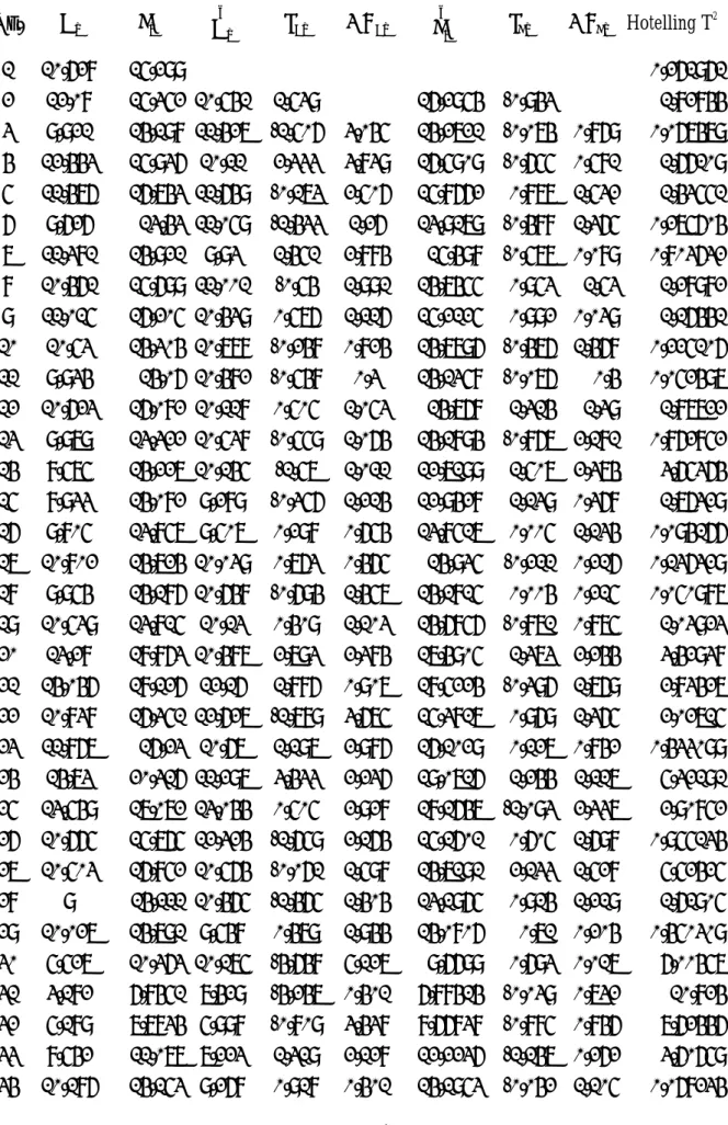
Table 1: The 100 observations for (Xt,Yt) No. Xt Yt ^ t X eXt MRXt ^ t Y eYt MRYt Hotelling T 2 1 10.628 15.299 0.261961 2 12.08 15.352 10.541 1.539 16.2954 -0.943 1.82844 3 9.921 14.198 11.427 -1.506 3.045 14.2721 -0.074 0.869 0.067479 4 12.443 15.936 10.11 2.333 3.839 16.5909 -0.655 0.581 1.66109 5 11.476 16.743 11.649 -0.173 2.506 15.8662 0.877 1.532 1.43551 6 9.626 13.43 11.059 -1.433 1.26 13.9179 -0.488 1.365 0.275604 7 11.381 14.921 9.93 1.451 2.884 15.498 -0.577 0.089 0.803632 8 10.461 15.699 11.001 -0.54 1.991 14.7455 0.953 1.53 1.28982 9 11.015 16.205 10.439 0.576 1.116 15.2125 0.992 0.039 1.16441 10 10.53 14.304 10.778 -0.248 0.824 14.7796 -0.476 1.468 0.225106 11 9.934 14.06 10.482 -0.548 0.3 14.1358 -0.076 0.4 0.052497 12 10.623 16.082 10.118 0.505 1.053 14.768 1.314 1.39 1.87722 13 9.979 13.322 10.538 -0.559 1.064 14.1894 -0.867 2.181 0.862852 14 8.575 14.227 10.145 -1.57 1.011 12.7199 1.507 2.374 3.65364 15 8.933 14.082 9.289 -0.356 1.214 12.9428 1.139 0.368 1.76329 16 9.805 13.857 9.507 0.298 0.654 13.8517 0.005 1.134 0.094166 17 10.802 14.724 10.039 0.763 0.465 14.935 -0.211 0.216 0.136329 18 9.954 14.186 10.648 -0.694 1.457 14.1815 0.004 0.215 0.050987 19 10.539 13.815 10.13 0.409 1.103 14.6856 -0.871 0.875 1.03923 20 13.28 18.863 10.487 2.793 2.384 17.4905 1.373 2.244 3.42938 21 14.046 18.126 12.16 1.886 0.907 18.5224 -0.396 1.769 2.83427 22 10.838 16.351 12.627 -1.789 3.675 15.3817 0.969 1.365 2.02715 23 11.867 16.23 10.67 1.197 2.986 16.1029 0.127 0.842 0.433099 24 14.73 20.316 11.297 3.433 2.236 19.0716 1.244 1.117 5.32191 25 13.549 17.072 13.044 0.505 2.928 18.1647 -1.093 2.337 2.90852 26 10.665 15.765 12.324 -1.659 2.164 15.1601 0.605 1.698 0.955134 27 10.503 16.852 10.564 -0.061 1.598 14.7191 2.133 1.528 5.52425 28 9 14.111 10.465 -1.465 1.404 13.1965 0.914 1.219 1.61905 29 10.027 14.791 9.548 0.479 1.944 14.0806 0.71 0.204 0.450309 30 5.527 10.363 10.175 -4.648 5.127 9.6699 0.693 0.017 6.00457 31 3.182 6.8451 7.429 -4.247 0.401 6.88414 -0.039 0.732 10.824 32 5.189 7.7834 5.998 -0.809 3.438 8.66838 -0.885 0.846 7.62446 33 8.542 11.077 7.223 1.319 2.128 12.2236 -1.147 0.262 3.60659 34 10.186 14.153 9.268 0.918 0.401 14.1953 -0.042 1.105 0.068234
35 11.759 16.465 10.272 1.487 0.569 15.9315 0.533 0.575 0.581365 36 12.995 17.886 11.232 1.763 0.276 17.3224 0.564 0.031 1.69991 37 9.992 14.632 11.986 -1.994 3.757 14.4319 0.2 0.364 0.302128 38 10.77 13.878 10.153 0.617 2.611 14.9208 -1.043 1.243 1.50637 39 14.828 18.779 10.628 4.2 3.583 19.0643 -0.285 0.758 4.30783 40 14.394 17.287 13.104 1.29 2.91 19.0218 -1.735 1.45 6.1185 41 14.791 20.068 12.839 1.952 0.662 19.3772 0.691 2.426 4.70693 42 16.439 20.57 13.082 3.357 1.405 21.0674 -0.497 1.188 7.66888 43 13.185 18.394 14.087 -0.902 4.259 17.9651 0.429 0.926 2.41323 44 13.339 17.293 12.102 1.237 2.139 17.8049 -0.512 0.941 1.95985 45 9.187 13.627 12.196 -3.009 4.246 13.6578 -0.031 0.481 0.43837 46 7.964 12.536 9.662 -1.698 1.311 12.0312 0.505 0.536 1.58162 47 9.408 14.211 8.916 0.492 2.19 13.3595 0.851 0.346 0.747548 48 12.457 16.071 9.797 2.66 2.168 16.5556 -0.485 1.336 1.45152 49 12.397 16.183 11.657 0.74 1.92 16.7907 -0.608 0.123 1.13994 50 12.294 17.234 11.621 0.673 0.067 16.6818 0.552 1.16 1.18754 51 13.809 18.75 11.558 2.251 1.578 18.1899 0.56 0.008 2.69616 52 9.138 12.392 12.482 -3.344 5.595 13.6548 -1.263 1.823 1.24111 53 11.672 16.144 9.632 2.04 5.384 15.7428 0.401 1.664 0.364923 54 9.558 12.92 11.178 -1.62 3.66 13.869 -0.949 1.35 0.891356 55 9.297 13.047 9.888 -0.591 1.029 13.4024 -0.355 0.594 0.435517 56 11.311 15.71 9.729 1.582 2.173 15.3965 0.314 0.669 0.186217 57 12.117 16.292 10.958 1.159 0.423 16.3985 -0.106 0.42 0.606532 58 8.349 11.451 11.45 -3.101 4.26 12.6997 -1.249 1.143 2.01656 59 8.611 11.309 9.151 -0.54 2.561 12.5985 -1.289 0.04 2.99173 60 6.333 9.2373 9.311 -2.978 2.438 10.3403 -1.103 0.186 4.75739 61 7.71 12.683 7.921 -0.211 2.767 11.4999 1.183 2.286 2.58507 62 9.881 13.232 8.761 1.12 1.331 13.8099 -0.578 1.761 0.856342 63 8.554 14.261 10.086 -1.532 2.652 12.6892 1.572 2.15 3.88636 64 7.856 13.941 9.276 -1.42 0.112 11.8615 2.079 0.507 6.37424 65 7.393 11.388 8.85 -1.457 0.037 11.3303 0.058 2.021 1.89787 66 9.952 13.376 8.567 1.385 2.842 13.8502 -0.474 0.532 0.712481 67 11.785 16.721 10.129 1.656 0.271 15.9344 0.787 1.261 0.892642 68 7.955 12.87 11.247 -3.292 4.948 12.2735 0.597 0.19 2.16575 69 10.105 13.716 8.91 1.195 4.487 14.0577 -0.342 0.939 0.40841 70 12.249 16.361 10.222 2.027 0.832 16.4146 -0.054 0.288 0.730034 71 11.606 14.716 11.53 0.076 1.951 15.9773 -1.261 1.207 1.90121 72 13.263 17.526 11.138 2.125 2.049 17.5757 -0.05 1.211 1.66926
73 10.734 13.361 12.149 -1.415 3.54 15.2011 -1.84 1.79 3.05212 74 8.514 12.519 10.606 -2.092 0.677 12.7323 -0.213 1.627 0.76164 75 7.407 10.708 9.251 -1.844 0.248 11.4076 -0.7 0.487 2.48831 76 8.834 13.891 8.576 0.258 2.102 12.7313 1.16 1.86 1.62151 77 10.729 12.996 9.447 1.282 1.024 14.7686 -1.773 2.933 4.58101 78 10.645 16.161 10.603 0.042 1.24 14.8675 1.294 3.067 2.051 79 12.395 16.656 10.552 1.843 1.801 16.6135 0.043 1.251 0.80049 80 13.064 16.264 11.62 1.444 0.399 17.4533 -1.189 1.232 3.04521 81 12.313 18.307 12.028 0.285 1.159 16.7649 1.542 2.731 4.11424 82 10.933 14.818 11.57 -0.637 0.922 15.3094 -0.491 2.033 0.194493 83 10.984 15.465 10.727 0.257 0.894 15.2269 0.238 0.729 0.137442 84 11.954 16.993 10.759 1.195 0.938 16.204 0.789 0.551 1.14789 85 7.733 12.331 11.35 -3.617 4.812 12.0667 0.264 0.525 1.879 86 8.273 10.935 8.775 -0.502 3.115 12.1996 -1.265 1.529 3.32225 87 8.611 13.124 9.104 -0.493 0.009 12.5909 0.533 1.798 0.898021 88 6.975 9.2197 9.311 -2.336 1.843 10.9837 -1.764 2.297 6.09336 89 9.978 12.828 8.312 1.666 4.002 13.8353 -1.007 0.757 2.1332 90 9.311 13.957 10.145 -0.834 2.5 13.4579 0.499 1.506 0.576574 91 10.411 15.282 9.738 0.673 1.507 14.4952 0.787 0.288 0.544448 92 8.701 13.029 10.409 -1.708 2.381 12.8881 0.141 0.646 0.681223 93 9.532 12.844 9.366 0.166 1.874 13.5557 -0.712 0.853 0.995131 94 8.606 12.964 9.873 -1.267 1.433 12.7081 0.256 0.968 0.772487 95 11.91 16.068 9.308 2.602 3.869 15.93 0.138 0.118 0.472838 96 9.451 13.283 11.324 -1.873 4.475 13.7845 -0.501 0.639 0.309009 97 9.43 14.392 9.823 -0.393 1.48 13.5253 0.867 1.368 1.0219 98 10.717 14.733 9.81 0.907 1.3 14.8136 -0.081 0.948 0.065452 99 10.878 13.413 10.596 0.282 0.625 15.0999 -1.687 1.606 3.47223 100 9.282 13.861 10.694 -1.412 1.694 13.5151 0.346 2.033 0.514682
Table2: Monitoring data for 51 observations (Xt,Yt) No. Xt Yt eXt eYt Hotelling T
2
2 11.0785 17.242 -2.03904 1.54197 1.85225 3 8.1424 11.869-2.67391-0.52364 0.77915 4 7.03365 11.6-1.99104 0.60294 1.14299 5 8.67484 11.702 0.32671-0.83271 1.27424 6 11.4983 15.081 2.1487-0.44229 0.280616 7 10.0398 14.494 -1.03264 0.15952 0.133074 8 6.79646 11.333-3.38604 0.39033 1.25318 9 6.94004 11.603-1.26336 0.82952 1.22572 10 9.6339 12.773 1.34289-0.71428 0.898015 11 13.6541 18.495 3.71926 0.71815 0.385109 12 17.4463 22.534 5.0584 0.56693 2.17794 13 14.6894 17.292 -0.01255-2.27823 2.15758 14 11.6981 17.334 -1.32156 1.02873 0.937439 15 16.0649 20.263 4.87048-0.13013 1.13374 16 10.826 14.579 -3.033-0.98555 0.186723 17 9.32026 12.745 -1.34195-0.80381 0.658145 18 10.4651 15.511 0.72163 0.96057 0.358845 19 5.41638 17.061 -5.0256 7.46 31.2008 20 12.2433 15.921 4.88207-0.03475 0.246105 21 22.0627 27.179 10.5356 0.72133 6.28831 22 23.9243 29.128 6.40544-0.14516 8.65909 23 21.0305 26.304 2.37572-0.24834 5.30496 24 12.5512 17.328 -4.33782-0.44572 0.168742 25 7.09018 10.02 -4.62477-1.45987 2.01101 26 5.32633 7.6617 -3.0563-1.52251 4.02275 27 8.62114 12.277 1.31482-0.03859 0.662756 28 5.98238 11.199-3.33444 1.20951 2.16352 29 4.52262 8.5559 -3.18403 0.28443 2.68066 30 9.69682 12.971 2.88092-0.34538 0.73004 31 15.0966 18.451 5.12338 -0.7777 1.2181 32 18.2478 23.131 4.97965 0.22152 2.59025 33 15.9519 20.10.760898-0.81316 1.08825 34 13.5524 17.185 -0.2376-1.10083 0.483099 35 12.8579 17.305 0.53198-0.05297 0.105075 36 15.8267 20.742 3.92465 0.47576 1.17349 37 11.222 14.831 -2.49172-1.10705 0.263398 38 10.7933 13.2 -0.11051 -1.8632 1.94094 39 9.77218 14.538 -0.8701 0.53974 0.286646
40 13.3735 19.007 3.35434 1.49785 1.09341 41 10.2868 15.206 -1.92995 0.44244 0.289896 42 7.68878 12.602 -2.64441 0.74115 1.01933 43 10.8339 14.315 2.08599-0.44718 0.384301 44 9.35976 13.115-1.30728-0.47404 0.403899 45 8.48772 11.907 -1.2798 -0.665 0.89113 46 12.514 16.082 3.27862-0.44192 0.354617 47 16.6993 19.763 5.007-1.34428 2.35491 48 12.1259 16.016 -2.12015-0.91217 0.115966 49 10.1841 14.25 -1.27134-0.28985 0.12498 50 6.72467 11.253-3.54587 0.36829 1.28809 51 8.69571 12.3510.536117-0.17507 0.640824 ACKNOWLEDGMENTS
Support for this research was provided in part by the National Science Council of the Republic of China, grant No. NSC-91-2118-M-004-008.
REFERENCE
1. Abraham, B. and Kartha, C.P.(1979). "Forecast stability and control charts”. ASQC Technical Conference Transactions. American Society for Quality Control, Milwaukee, WI. Pp. 675-685.
2. Alwan, L.C. (1991),”Autocorrelations: Fixed and Versus Variable Control Limits”. Quality Engineering 4, pp.167-188.
3. Alwan, L.C. and Radson, D. (1992). “ Time-Series investigation of subsample mean chart”. IIE Transactions 24, pp.66-80.
4. Alwan, L.C. and Roberts, H. V. (1988). " Time-Series modeling for statistical process control”. Journal of Business and Economic Statistics 6, pp.87-95.
5. Berthouex, P. M., Hunter, W. G. and Pallesen, L. (1978). “ Monitoring sewage treatment plants: Some quality control aspects”. Journal of Quality Technology 10. pp.139-149.
6. Delves, L. M. and Mohamed, J.L. (1985). Computational Methods for Integral Equations. Cambridge University Press, New York, NY.
7. Dooley, K.J. Kapoor, S. G., Dessouky, M. I., and Devor, R. E. (1986). “ An integrated quality systems approach to quality and productivity improvement in continuous manufacturing processes”. Transactions of the ASME Journal of Engineering for Industry 108. pp. 322-327.
8. Ermer, D.S. (1980). "A control chart for dependent data". ASQC Technical Conference Transactions. American Society for Quality Control, Milwaukee, WI. pp.121-128.
observations”. The Canadian Journal of Chemical Engineering 69, pp. 48-57.
10. Kramer, H. and Schmid, W. (1997). “ Control charts for time series”. Nonlinear Analysis 30, pp. 4007-4016.
11. Lin, W.S. and Adams, B. M. (1996). “ Combined control charts for forcast-based monitoring schemes”. Journal of Quality Technology 28, pp. 289-301.
12. LONGNECKER, M. T. and RYAN, T. P. (1992). “Charting Correlated Process Data”. Technical Report No.166. Department of Statistics. Texas A & M University. Collage Station, TX.
13. Lu, C. and Reynolds, M. (1999). “EWMA control charts for monitoring the mean of autocorrelated processes.”, Journal of Quality Technology, Vol.31, pp.166-188.
14. Montgomery, D. C. (1996). Introduction to Statistical Quality Control, 3rd ed. John Wiley & Sons, New York, NY.
15. Montgomery,, D. C. and Mastrangelo, C. M. (1991). “Some Statistical Process Control Methods for Autocorrelated data”. Journal of Quality Technology 23, pp. 179-193.
16. Padgett, C. S.; Thombs, L. A.; and Padgett, W.J. (1992). “On the
α
-risks for Shewhart Control Charts”. Communications in Statistics-Simulation and Computation 21, pp. 1125-1147.17. Runger, G. C.; Willemain, T.R.; and Prabhu, S. (1995). “Average Run Lengths for CUSUM Control Charts Applied to Residuals”. Communications in Statistics-Theory and Methods 24, pp. 273-282.
18. Schmid, W. (1995). “On the Run Length of a Shewhart Chart for Correlated Data”. Statistical Papers 36, pp. 111-130.
19. Schmid, W. (1997a). “CUSUM Control Schemes for Gaussian Processes”. Statistical Papers 38, pp. 191-217.
20. Schmid, W. (1997b). “On EWMA Charts for Time Series” in Frontiers of Statistical Quality Control edited by H. J. Lenz and P.-Th. Wilrich. Physica-Verlag, Heidelburg.
21. Sshmid, W. and Schone, A. (1997). “Some Properties of the EWMA Control Chart in the Presence of Autocorrelation”. Annals of Statistics 25, pp. 1277-1283.
22. Timmer, D. H.; Pigantkiello. J. JR.; and Longnecker, M. (1998). “The Development and Evaluation of CUSUM-Based Control Charts for an AR(1) Process”. IIE Transactions 30, pp. 525-534.
23. Vander Well, S. A. (1996). “Modeling Processes That Wander Using Moving Average Models”. Technometrics 38, pp. 139-151.
24. Wade, R. and Woodall, W., “A Review and Analysis of Cause-Selecting Control Charts,” Journal of Quality Technology, 25,.161-169 (1993).
25. Wardell, D. G.; Moskowitz, H.; and Plante, R. D. (1992). “Control Charts in the Presence of Data Correlation”. Management Science 38, pp. 1084-1105.
26. Wardell, D. G.; Moskowitz, H.; and Plante, R. D. (1994) “Run Length Distributions of Special-Cause Control Charts for Correlated Processes”. Technometrics 36, pp. 3-17.
27. Yashchin, E. (1993). “Performance of CUSUM Control Schemes for Serially Correlated Observations”. Technometrics 35, pp. 37-52.
Data”. Journal of Applied Statistics 24, pp. 363-380.
29. Zhang, G., “A New Type of Control Charts and a Theory of Diagnosis with Control Charts,” World Quality Congress Transactions, American Society for Quality Control, Milwaukee, WI, 75-85 (1984).
CONTROL FOR THE AUTOCORRELATED OBSERVATIONS
Su-Fen Yang Chung-Ming Yang Department of Statistics Department of Insurance National Chengchi University Ling-Tung College
Taipei, 116, Taiwan Taichung, 408,Taiwan E-mail: [email protected]
ABSTRACT
The observations from the process output are always assumed independent when using a control chart to monitor a process. However, for many processes their observations are autocorrelated and including the measurement error due to the measurement instrument. This autocorrelation and measurement error can have a significant effect on the performance of the processes control. This paper considers the problem of monitoring the mean of a quality characteristic X on the first process and the mean of a quality characteristic Y on the second process, in which the observations X can be modeled as an ARMA model and observations Y can be modeled as an transfer function of X since the state of the second process is dependent on the state of the first process. To effectively distinguish and maintain the state of the two dependent processes with measurement errors, the Shewhart control chart of residual and the cause-selecting control chart based on residuals are proposed. The performance of the proposed control charts is evaluated by the rate of true alarm or false alarm. From numerical analysis, it shows that the performance of the proposed control charts is significantly influenced by the variation of measurement errors. Application of the proposed control charts is illustrated through a numerical example.
Key Words: Autocorrelated observations, dependent processes, cause-selecting control chart,
measurement error variation.
1. INTRODUCTION
Control charts are first proposed by Shewhart (1931), and become effective tools for
A basic assumption in applications of control charts is that observations from the process at
different times are independent random variables. However, the independence assumption is often
violated for processes in chemical and pharmaceutical industries. Observations from these processes
are always autocorrelated. When the control charts developed under the independence assumption,
the autocorrelated process results in decreasing the in-control average run length (ARL). For
effective monitoring the autocorrelated processes, one popular developed approach is to
constructing control charts using the residuals from the time series model to the process data (see
Abraham and Kartha (1979), Alwan (1991), Alwan and Roberts(1988), Berthouex, Dooley, Kapoor,
Dessouky and Delves (1986), Ermer (1980), Harris and Ross (1991), Montgomery (1996),
Montgomery and Mastrangelo (1991), and Wardell, Moskowitz, and Plante (1992, 1994)). The
properties of the proposed residual charts and their performance are investigated by Harris and Ross
(1991), Longnecker and Ryan (1992),Yashchin (1993),Kramer and Schmid (1997), Schmid
(1995),Lin and Adams (1996), Schmid (1997a), Padgett, Thombs and Padgett (1992), Runger,
Willemain and Prabhu (1995), Vander Weil (1996), Timmer, Pignatiello and Longnecker (1998),
Schmid (1997b) ,Zhang (1998), Schmid and Schone (1997), Alwan and Roberts (1988) and Lu and
Reynolds (1999).
Much of the paper on the performance of control charts based on residuals has focused on the
Shewhart control chart of residuals.
The above autocorrelated processes articles assume that the imprecise measurement devices on
statistical process control tools could be seriously affected when the process measurement includes
the error due to the measurement instrument. The effect of measurement error on the operating
characteristics of an X chart, in cases where only the process mean shifts, is discussed by Bennett
(1954), Mizuno (1961), Abraham(1977), Mittag (1993) and Mittag and Stemmann (1993).
Kanazuka (1986) and Mittag (1995) investigate the effect of measurement error on the power
characteristics of the X -R control chart where both the process mean and process spread change.
Mittag and Stemann (1998) extend the results of Mittag (1995), referring to the X -S control chart.
Rahim (1985) analysis the effects of imprecise measurement devices on the design parameters of
the economic X control chart. Yang (2002) investigates the effect of measurement error on the
design parameters of the economic asymmetric X and S control charts.
The above control charts articles consider a single process control. Today, many industrial
products are produced in several dependent processes. Consequently, it is not appropriate to monitor
these processes by utilizing a control chart for each individual process. Zhang (1984) proposes the
simple cause-selecting chart to monitor the second process of the two dependent processes. Wade
and Woodall (1993) review the basic principles of the cause-selecting chart for two dependent
processes and modify Zhang’s approach, and give an example to illustrate the use of the individual
X chart and the simple cause-selecting chart. It is shown that their approach is better than that of
Zhang for the dependent processes control. However, the statistical process control approach to
effectively distinguish and monitor the dependent processes for autocorrelated observations
In this paper, process measurements with measurement error used in construction of Shewhart
control chart of residuals and cause-selecting control chart are developed. The proposed control
charts can be effectively used to distinguish which process mean is out of control, and the effect of
imprecise measurement on the performance of the proposed control charts for monitoring the two
dependent processes is also investigated. Finally, application of the proposed control charts is
demonstrated through an example. Numerical examples illustrate the effects of imprecise
measurement on the proposed control charts.
2. PROBLEM STATEMENT
A possible industrial situation is taken to illustrate the effects of imprecise measurement on
the performance of the two proposed control charts, which are respectively used to monitor the
process means for autocorrelated observations on two dependent processes. In a production
system, suppose that there are two dependent processes, which may have two types of failure
mechanisms. One type of the failure mechanism occurs only on the first process and shifts the
mean of the quality variable (X), while the other type occurs only on the second process and shifts
the mean of the quality variable (Y). The quality variable Y is influenced by the quality variable
X since the processes are dependent. The measurement process is considered, and it has a
variance for a measurement device is employed for later measurements. Some quality engineers
would like to develop appropriate control charts to monitor the process means on the two dependent
process control policy under the measurement error? That is, what are the control charts, how the
measurement error affects the performance of the proposed control charts.
The solutions of these problems are as follows.
(1) A measurement device having measurement dispersion is investigated and the model of
measurement error for the first process is determined. An appropriate time series model of the
quality variable X is determined, since its observations are autocorrelated. Based on the
in-control distribution of residuals (X −X^ , the individual residual control chart can be set up to monitor the process mean of the first process.
(2) A measurement device having measurement dispersion is investigated and the model of
measurement error for the second process is determined. An appropriate transfer function for
quality variable Y and quality variable X is determined, since the quality variable Y is
influenced by the quality variable X and correlated on time. Based on the in-control distribution
of residual (Y −Y^ ) of the transfer function, the cause-selecting control chart can be set up to monitor the process mean of the second process.
(3) The two proposed control charts are used to distinguish and detect the shifts of process mean on
the two dependent processes, and the detecting ability of the proposed control charts for
different measurement dispersion is calculated and compared. Based on the analysis results,
appropriate control policy can be proposed by the quality engineers.
3. DESCRIPTION OF PROCESSES
two dependent processes for autocorrelated observations with measurement errors. Before
describing how to derive the two statistical control charts, the assumptions of the two dependent
production processes behavior are given as follows.
3.1Assumptions and Notation
Assumptions
(5) The production has two dependent processes, say the process 1 and the second process is called
the process 2. The process 1 and the process 2 are dependent. So the quality variable XT
produced by the process 1 will affect the quality variable YT produced by the process 2. A pair
of true observations (xTt,yTt) are sampled from the end of the process 2 every h time unit of
sampling interval,t =1,2,3,...
(6) For autocorrelated true observationsxTtat process 1, it is assumed that quality variableXTcan be
written as an AR(1) model at time t with process meanξX, that is XTt =(1−φ1)ξX +φ1XT(t−1)+at ,t=1,2,...., (1)
where φ1 is the AR parameter satisfying |φ1|<1. The at’s are assumed to be independent normal random variables with mean 0 and variance 2
a
σ . The starting value, XT0, is assumed
following a normal distribution with mean εXand variance 2
1 2 2 1 φ σ σ − = a XT .
Since XT affects YT, we assume the model relating the two variables can be written as a
simple transfer function. That is
,.... 2 , 1 , ' ) 1 ( ' 1 ' 0 ' + + + = =C V X V X − N t YTt Y Tt T t t , (2) where ' Y
C is a constant and where '
t
with mean 0 and variance 2
'
N
σ .
(7) When one failure mechanism occurs only in the process 1, it will shift the mean of XT. This
will also cause the mean of YT shifts. When the other failure mechanism occurs only in the
process 2, then it will shift the mean of YT and the mean of XT is unchanged.
(4) It is assumed that the measurement process for XT has a variance, 2
ε
σ
X , for a measurement device is employed for later measurements. That is, the distribution of the measurement error(
ε
X) is illustrated asε
X ~N(0, 2ε
σ
X ). Hence, the distribution of the observed process quality variable ( X ) with measurement error (ε
X) is illustrated as X= XT +ε
X.(5) It is assumed that the measurement process for YT has a variance, 2
ε
σ
Y , for a measurementdevice is employed for later measurements. That is, the distribution of the measurement error
(
ε
Y) is illustrated asε
Y~N(0, 2ε
σ
Y ). Hence, the distribution of the observed process qualityvariable (Y ) with measurement error (
ε
Y) is illustrated as Y=YT +ε
Y .(6) Two control charts are proposed to monitor the two dependent processes effectively.
(7) The time to sampling and charting one item is very small and negligible.
3.2. The Time Series Model For Autocorrelated Processes
Time series model, especially AR(1) model, has been widely used to model many types of
processes. For process 1, the AR(1) process observed with measurement errors is equivalent to an
ARMA(1,1) process (Box, Jenkins, and Reinsel (1994). That is, X = XT +
ε
X , XT is independent of the εX, and X is an ARMA(1,1) model. When the process 1 is in-control, the ARMA(1,1) model at time t is expressed as1 1 1 1 0 1) 1 ( − + − + − − = X t t t t X X φ ξ φ γ θ γ , (3) where ~ (0, 2) r t NID σ
γ , θ1 is MA parameter, and φ1 is AR parameter.
Parameters φ1 ,θ1 and 2
r
σ in the ARMA(1,1) model in terms of the parameters φ1 , 2
a
σ and 2 ε
σX in the AR(1) model plus random error model. If φ1 >0 and
2 ε
σX >0, then the ARMA(1,1) model parameters θ1 and
2
r
σ can be obtained from the AR(1) plus error parameters using
4 ) ) 1 ( ( 2 1 2 ) 1 ( 2 2 1 2 2 1 2 2 1 2 2 1 2 1 − + + − + + = ε ε ε ε σ φ σ φ σ σ φ σ φ σ θ X X a X X a (4) and 1 2 1 2 θ σ φ σ Xε r = (5)
(Reynold, Arnold, and Baik (1996)).
If 2
a
σ , 2 ε
σX and φ1 are known, then θ1 and 2
r
σ are known. When the process 1 is in control the minimum mean square error forecast made at time t-1 for time t is
1 ^ 1 1 1 ^ 0 1 ^ ^ ) 1 ( − + − − − = X t t t X X φ ξ φ θ γ , (6) ^ t t Xt X X e = − (7) Xt
e is the residual at time t, ~ (0 , 2)
r
σ
N
eXt .
Suppose that a failure mechanism would cause a step change from ξX0to ξX1in the process
mean between time t=τ−1and τ . The expectations of the residual for various times are
∞ → + = − = + = − + − − − − = = , ) ( -1 -1 ,.... 2 , 1 , 0 , ) ( -1 1 ) ( , 2 1 0 ) ( 0 X1 1 1 0 X1 1 1 1 1 1 l l t l l t ,... , τ τ t e E X X l Xt τ ξ ξ θ φ τ ξ ξ θ φ θ φ θ (8)
The residuals are uncorrelated and normally distributed with variance 2
a
expectation of a residual after the shift occurs is a decreasing function of the time after the shift.
Hence, the rate of a true alarm from the control chart of residuals on the process 1 is the lowest for
the sample immediately after the shift, and this rate of a true alarm continually increases and
converges to a constant over time as the forecast adapts to the shift.
In process 2, a linear transfer function also presents the relationship between Y and
X since they are dependent over time. The transfer function plus random error (
ε
Y) is expressedas ,.... 2 , 1 , ) 1 ( 1 0 + + + = + =C V X VX − N t Yt Y t t t εYt (9) where ~ (0, 2) N t NID N σ , and ~ (0, 2 ) ε ε σ εY NID Y .
When the process 2 is in control, the estimate for equation (9) is
Y^t =C^y+V^0 Xt +V^1Xt−1, (10)
and the residual at time t is
^ t t Yt Y Y e = − , (11) where ~ (0 , 2 ) Y 2 N σ ε σ + N eYt .
Suppose that another failure mechanism would cause a step change from ξY0to ξY1in the process
mean between time =τ'−1
t and τ'. The expectations of the residual for various times are
,.... 2 , 1 , 0 , , 2 1 0 ) ( ' ' 0 Y1 ' ' = + = = − − − = = l l t t ,... , t e E Y Yt τ τ ξ ξ τ τ (12)
The residuals are uncorrelated and normally distributed with variance 2 2 ε
σ
σN + Y . Note that the shift of process mean only appears at time τ' after the shift.
4. CONSTRUCTING CONTROL CHARTS
To effectively distinguish and monitor the two dependent processes, two Shewhart control
charts based on residuals, eXand eY, are constructed. The control limits of the Shewhart control
charts are dependent on the in-control distribution of eXand eY, respectively. Since the in-control
distribution of eX is ~ (0 , )
2 r
σ
N
eXt , hence the control limits of the Shewhart control chart based on
X
e , using to monitor the process 1, are as follows.
r eX UCL =3σ 0 = X e CL r eX LCL =−3σ .
From equation (5), we know that
σ
γ is a function of measurement error variation,σ
Xε, for process 1. Hence, the control limits of the Shewhart control chart of eX include the variation ofmeasurement error. It indicates that the performance of the Shewhart chart is influenced by the
variation of measurement error.
If the parameterσris unknown then
2 d MReX is replaced, where 1 2 − =
∑
= m MR MR m t eXt eX , 2 ) 1 ( |, 23 |e e t , ,...,m, dMReXt = Xt − Xt− = is the factor of constructing control charts.
For process 2, the in-control distribution of eY is ~ (0 , )
2 Y 2 N σ ε σ + N
eYt , hence the control
limits of the Shewhart control chart based on eYare as follows.
) ( 3 2 2 ε σ σ Y eY N UCL = +
0 = Y e CL ) ( 3 2 2 ε σ σ Y eY N LCL =− + .
The control limits of the Shewhart control chart of eYinclude the variation of measurement
error,e , for process 2. It indicates that the performance of the Shewhart chart of Yt eY is
influenced by the variation of measurement error.
If the parameter 2 2 ε σ σN + Y is unknown then 2 d MReY is replaced, where 1 2 − =
∑
= m MR MR m t eYt eY , . 3 2 |, |e e ( 1) t , ,...,m MReYt= Yt− Yt− =To monitor the two processes using the proposed control charts, a pair of observations (X ,t Yt)
is sampled at the end of the process 2. The plotted statistics eXand eY are calculated, and plotted
on the proposed control charts, respectively. If no one signal any control charts, it indicates the two
processes are all in control. If only a signal from the Shewhart control chart of eX, it indicates
process 1 is out of control. The quality engineer has to search and remove the occurred special
cause. If only a signal from the Shewhart control chart of eY, it indicates process 2 is out of control.
The quality engineer has to search and remove the occurred special cause. If both signals from the
Shewhart control chart of eX and Shewhart control chart ofeY, it indicates process 1 and process 2
are out of control. The quality engineer has to search and remove the special causes on the
out-of-control processes.
The performance of the proposed control charts is evaluated by the rate of false alarm when the
processes are in control, and the rate of true alarm (or power) when the processes are out of control.
For process 1, the rate of false alarm for the Shewhart chart of eXis 370.4, and the same to the
Shewhart chart of eYat process 2. To monitor the two dependent processes, two developed charts
are used simultaneously. Hence the rate of at least one false alarm for the two charts is 0.0054,
that is 1-0.9973x0.9973. To calculate the rate of true alarm for the two charts, we have to compute
the rates of true alarm from the Shewhart chart of eX and Shewhart chart of eY, respectively. Let
the rate of true alarm from the Shewhart chart of eXat time t isPs , and the rate of true alarm from t
the Shewhart chart of eYat time t isPc , then t
,.... 2 , 1 , 0 , ), ) ( -1 1 ) ( 3 ( ) ) ( -1 1 ) ( 3 ( ) ) ( -1 1 ) ( | 3 3 Pr( 0 X1 1 1 1 1 1 0 X1 1 1 1 1 1 0 X1 1 1 1 1 1 = + = − + − − + − Φ + − + − − − − Φ = − + − − − < > = l l t e or e Ps X l S X l S X l Xt Xt t τ σ ξ ξ θ φ θ φ θ σ ξ ξ θ φ θ φ θ ξ ξ θ φ θ φ θ σ σ γ γ γ γ (13) ' 0 1 0 1 0 1 ), ) ( ) ( 3 ( ) ) ( ) ( 3 ( )) ( | ) ( 3 ) ( 3 Pr( τ σ σ ξ ξ σ σ ξ ξ ξ ξ σ σ σ σ ε ε ε ε = + − + − Φ + + − − − Φ = − + − < + > = t e or e Pc Y N Y Y C Y N Y Y C Y Y Y N Yt Y N Yt t (14) Alternatively, ,.... 2 , 1 , 0 , ), ) ( -1 1 ) ( 3 ( ) ) ( -1 1 ) ( 3 ( ) ) ( -1 1 ) ( | 3 3 Pr( 0 X1 1 1 1 1 1 2 0 X1 1 1 1 1 1 2 0 X1 1 1 1 1 1 2 2 = + = − + − − + − Φ + − + − − − − Φ = − + − − − < > = l l t MR d MR d d MR e or d MR e Ps eX X l S eX X l S X l eX Xt eX Xt t τ ξ ξ θ φ θ φ θ ξ ξ θ φ θ φ θ ξ ξ θ φ θ φ θ (15)
' 0 1 2 0 1 2 0 1 2 2 ), ) ( 3 ( ) ) ( 3 ( )) ( | 3 3 Pr( τ ξ ξ ξ ξ ξ ξ = − + − Φ + − − − Φ = − − < > = t MR d MR d d MR e or d MR e Pc eY Y Y C eY Y Y C Y Y eY Yt eY Yt t (16)
where ΦSand ΦC are the cumulative standard normal probabilities, respectively.
Note that the rate of true alarm from the Shewhart chart of eXincreasing and converges to a
constant over time, but not for the Shewhart chart of eY. Hence the rates of true alarm from the
two charts will be increasing over time, once the process 1 is out of control.
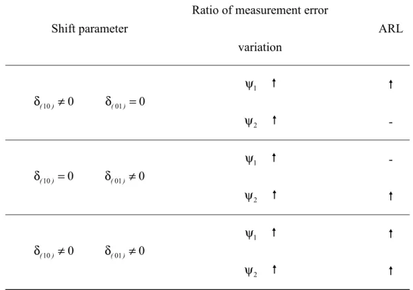
The rate of true alarm from the Shewhart chart of eXor the Shewhart chart of eY is also dependent
on the variation of measurement error. From the equations (13) and (14), we find that the lager the
variation of measurement errors leads to the larger rate of true alarm from the proposed control
chart when any one of the processes is out of control.
There are four situations for the out-of-control process. The four situations and the rate of true
alarm of the two charts are described as follows.
(5) The process 1 is out of control after time τ−1 but the process 2 is in control. The rate of true alarm (Psc ) of the two charts is t
Psct =1−(1−Pst), t =
τ
+l, l =0,1,2,3,....(6) The process 1 is in control but the process 2 is out of control after time
τ
'−1. The rate of true alarm (Psc ) of the two charts is tPsc =1−(0.9973), t =
τ
'.t
(7) The process 1 is out of control after timeτ−1, and the process 2 is out of control after time
τ
' −1, whereτ
<τ
'. The rate of true alarm (t
.... 3 , 2 , 1 , ), 1 ( 1 , ), 1 )( 1 ( 1 ), 1 ( 1 ' ' ' = < + − − = − − − < ≤ − − = l t l Ps t Pc Ps t Ps Psc t t t t t
τ
τ
τ
τ
(8) The process 1 is out of control after timeτ"−1, and the process 2 is out of control after time
τ
' −1, whereτ
" >τ
'. The rate of true alarm (t
Psc ) of the two charts is
. ) 1 ( 1 , ) 1 ( 1 " '
τ
τ
≥ − − = − − = t Ps t Pc Psc t t t 甲、 NUMERICAL EXAMPLES6.1 Performance of the Proposed Control Charts
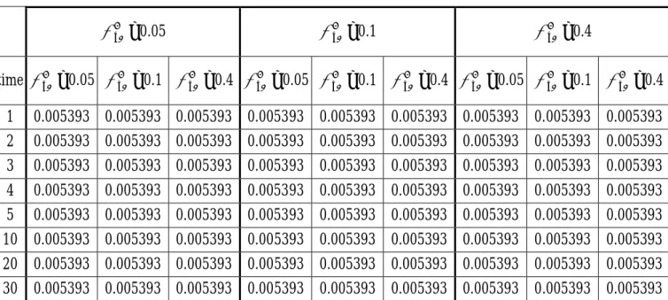
The performance of the proposed control charts under various variations measurement error will be evaluated by the rate of false alarm or the rate of true alarm. The rate of false alarm for in-control processes or the rate of true alarm for out-of-control processes depends on the values of
parameters φ1, 2 a σ , 2 ε σY , 2 ε
σ
X , σN2 ,ξX1−ξX0 and ξY1−ξY0 . We fix φ1=0.6, 2 a σ =0.5, and 2 Nσ =0.5, but let ξX1−ξX0=0, 1, 2, ξX1−ξX0=0, 1, 2, σX2ε=0.05, 0.1, 0.4, and 2
ε
σY =0.05, 0.1, 0.4, respectively. The numerical values of rate of false alarm or rate of true alarm for the proposed charts are illustrated in the Table 1 ((1)~(6)). We find that the rate of false alarm keeps 0.005393 when both the processes are in control no matter what the variation of measurement error. For fixed variation of measurement error in the in-control process 2, the larger variations of measurement errors in the out-of-control process 1 lead to small rates of true alarm. That is, the imprecision measurement may seriously affect the ability of the proposed control charts to detect process disturbances quickly. For fixed variation of measurement error in the process 2 and fixed variation of measurement error in the out-of-control process 1, the rate of true alarm of the proposed charts decreases over time. That is, the detection ability of the proposed charts is largest after a failure mechanism occurs, but decreases and converges to constant over time. For fixed variation of measurement error in the process 1, the larger variations of measurement errors in the out-of-control
process 2 lead to small rates of true alarm of the proposed charts. For fixed variation of measurement error in the process 1 and fixed variation of measurement error in the out-of-control process 2, the rate of true alarm of the proposed charts increases dramatically right the time after the failure mechanism (time 4 in Table 1(3), and time 11 in Table 1(6)) occurs but back to normal from next time (time 5 in Table 1(3), and time 12 in Table 1(6)). All indicates that the imprecision measurement may seriously affect the ability of the proposed control charts to detect process disturbances quickly.
6.2 Application of the Proposed Control Charts
A quality engineer found that there is a large variability for the thickness of the thin golden
films. From the quality data analysis, he found that the thickness of the thin golden films (Y ) in the
process 2 was primarily affected by gold concentration ( X ) in the process 1. Two independent
machines, say machine 1 and machine 2, may failure and influence the mean of the gold
concentration and thickness respectively. However, for measuring X and Y , the process
measurement includes the error due to the measurement instrument. Since the unacceptable mean of
the thickness may be influenced by machine 1 or gold concentration. To effectively maintain the
variability of the gold concentration and thickness and distinguish which process is out of control,
two control charts should be constructed as described before. The performance of the proposed
control charts is influence by the variation of measurement errors, since the variation of
measurement errors is included in the control limits. To investigate the effects of variation of
measurement errors on the performance of the proposed control charts, the detecting ability of the
charts is compared under various variations of measurement errors.