James K. Hammitt
Department of Health Policy and Management and Center for Risk Analysis
Harvard School of Public Health Boston, Massachusetts USA
Jin-Tan Liu
Department of Economics National Taiwan University
Taipei, Taiwan and NBER September 2002
Corresponding author: James K. Hammitt, Harvard School of Public Health, 718 Huntington Ave., Boston, MA 02115-5924. Tel: 617 432 4030, Fax: 617 432 0190, E-mail: [email protected]
Acknowledgment: The survey instrument was developed with support from the US Environmental Protection Agency (CX827776-01-0). Survey administration was funded by the Taiwan National Science Council (NSC90-2415-H-002-030). We thank John Bennett, Maureen Cropper, Chris Leggett, and participants at the 2002 NBER Summer Institute for helpful comments.
We evaluate the effects of disease type and latency on willingness to pay (WTP) to reduce environmental risks of chronic, degenerative disease. Contingent-valuation data were collected from approximately 1,250 respondents in Taiwan. These data suggest the existence of a “cancer premium:” WTP to reduce risk of cancer is estimated to be about 30 percent larger than WTP to reduce risk of a similar chronic degenerative disease. The value of risk reduction also depends on the affected organ, environmental pathway, or payment mechanism: WTP to reduce the risk of lung disease due to industrial air
pollution is estimated to be twice as large as WTP to reduce the risk of liver disease due to contaminated drinking water. Finally, we find that WTP is insensitive to the latency period between exposure to environmental contaminants and manifestation of disease. This insensitivity suggests that respondents anticipate their value per statistical life will grow over time at a rate about equal to their discount rate.
Keywords: health risk, contingent valuation, willingness to pay, value per statistical life, cancer, latency, Taiwan
1. Intr oduction
Many environmental regulations are directed toward reducing risks of cancer and other disease. Yet most of the empirical literature on valuing health risk relies on
estimates of the compensating wage differentials that workers receive for bearing risks of fatal injury in the workplace (Viscusi, 1993). The applicability of these wage-differential estimates to changes in environmental health risks is uncertain. Environmentally-induced cancer and other diseases differ from occupational fatal injuries in several dimensions that may affect preferences. Two that may be of particular importance are (1) the
difference in latency between exposure to the hazardous condition and the manifestation of adverse health effects, and (2) dread or other factors that lead to greater fear of cancer than of other causes of fatality (Revesz, 1999; Sunstein, 1997). In addition, reflecting the great public attention given to cancer, there may be differences in concern about cancer and other degenerative, fatal diseases that can be caused by exposure to environmental contaminants.
We use contingent valuation (CV) to test for effects of disease type and latency on individual willingness to pay (WTP) to reduce risks of developing a fatal cancer or other chronic degenerative disease through exposure to environmental pollution. Because the consequences of developing cancer are more similar to those of other chronic
degenerative disease than they are to acute trauma in a workplace or other accident, our estimates of the effect of disease type on WTP are likely to understate any difference in WTP between cancer and trauma. Data were collected from 1,248 respondents in Taiwan. We find evidence that there is a statistically significant “cancer premium,” that WTP depends on the affected organ or environmental pathway, and that WTP is not significantly related to the latency of the disease.
In the following section, we provide an overview of the economic theory and previous empirical results concerning the effects of disease type and latency on
willingness to pay for reductions in mortality risk. The empirical methods are described in Section 3, results are in Section 4, and Section 5 concludes.
2. Economic Theor y of WTP to Reduce Mor tality Risk
The economic approach to valuing mortality risk was developed by Drèze (1962), Schelling (1968), and Jones-Lee (1974). The individual’s rate of tradeoff between wealth and risk in a specified time period (e.g., the current year) is characterized by his marginal rate of substitution between mortality risk p and wealth or income w. The marginal rate of substitution
dp dw
(holding utility constant) is called the “value per statistical life” (VSL). VSL is not a universal constant but varies by individual and circumstance. The standard economic model of preferences for wealth and mortality risk (Drèze, 1962; Jones-Lee, 1974; Weinstein et al., 1980) assumes that an individual’s welfare can be represented as
EU(p, w) = (1 – p) ua(w) + p ud(w) (1)
where p is the individual’s chance of dying during the current period and ua(w) and ud(w)
represent his utility as a function of wealth conditional on surviving and not surviving the period, respectively. The function ud(•) incorporates the individual’s preferences for
bequests and can incorporate any financial consequences of dying (such as medical bills or life-insurance benefits). In this one-period model, wealth and income are treated as equivalent, but the difference between them can be important in multi-period models.
The individual’s VSL is derived by differentiating equation (1) holding expected utility constant to obtain
( )
( )
(
) ( )
( )
Eu( )
( )
w w u w u p w u p w u w u dp dw VSL d a d a ′ ∆ = ′ + ′ − − = = 1 (2)where prime indicates first derivative. The numerator in equation (2) is the difference in utility between surviving and dying in the current period. The denominator is the
expected marginal utility of wealth, i.e., the utility associated with additional wealth conditional on surviving and dying, weighted by the probabilities of these events. Assuming that life is preferred to death and that greater wealth is preferred to less, both numerator and denominator are positive and so VSL is positive. If the marginal utility of wealth is non-negative, and greater in the event of survival than death (i.e., ua'(w) > ud'(w)
conditional on survival and on death (i.e., ua" ≤ 0, ud" ≤ 0), is a sufficient condition for
VSL to increase with wealth. Accounting for Latency
In equation (2), VSL is defined in terms of wealth and mortality risk in a single period. Many environmental risks are characterized by a latency period between the time an individual is exposed to an agent and the time when he may die from its toxic effect. Since preventive measures must be undertaken before the exposure occurs, there is often a need to determine WTP now to reduce the risk of fatality in a future period.
Standard economic theory suggests that the appropriate procedure to account for latency is to value the risk change using the VSL representing the individual’s value when the risk manifests, and to adjust for the time-value of money and the chance that the individual will die before then (Cropper and Sussman, 1990; Cropper and Portney, 1990). Formally, t t t t t sVSL r r WTP ∆ + = 1 1 , 0 (3)
where WTP0,t is the individual’s willingness to pay at time 0 for an increase of magnitude
∆rt in his survival probability at time t (conditional on surviving to t), r is the individual’s
opportunity cost of funds (the rate of return on investments), st is the probability he
survives from time 0 until time t, and VSLt is his VSL at time t. For example, assume that
pollution-control equipment that could be installed today would reduce an individual’s risk of dying from cancer by 1 chance in 100,000, that the cancer would prove fatal 20 years after exposure, that his VSL in 20 years will be $8 million, and that the individual can earn a 5 percent annual return on investments. In 20 years, he would be willing to pay $80 to reduce a contemporaneous fatality risk of 1 in 100,000. The amount he would be willing to pay now is the present value of $80, about $30 (= $80 x 1.05-20) times the probability of surviving the intervening 20 years, since the cancer-risk reduction is of no benefit in the event that he dies of other causes before the environmental pollutant could have killed him. In many cases, this survival factor is much less important than the discount factor. For the average American, the probability of surviving 20 years is greater
than 0.7 if the individual is younger than 55 (National Center for Health Statistics, 1998).1
The difference between an individual’s current and future VSL depends on two factors: he will be older, and the date will be later. Age affects VSL because the individual’s life expectancy, earnings, opportunities for spending on other goods, and other factors vary with the stage of the life cycle. Time or date affect VSL through secular changes in productivity, the availability of medical and other technologies for investing in longevity, and other factors. A number of theoretical and empirical studies have
examined the effects of age on VSL, but the effect of date has received little attention. Because of secular changes in productivity and other factors, the VSL at age 70 of a current 30 year old is unlikely to be equal to the current VSL of a 70 year old.
The effect of age has been examined in theoretical models and, to a limited extent, by empirical studies. Theoretical models (e.g., Shepard and Zeckhauser, 1984; Rosen, 1988; Ng, 1992) represent the individual’s lifetime utility as the expected present value of his utility in each time period. Utility within a period depends on consumption, which is limited by current income, savings and inheritance, and ability to borrow against future earnings. The individual seeks to maximize lifetime utility by allocating his wealth to consumption, savings, and reductions in current-period mortality risk.
Two factors influence the life-cycle pattern of VSL. First, the number of future life years at risk declines as one ages, so the benefit of surviving the current period (the numerator in equation (2)) declines. Second, the opportunity cost of spending on risk reduction (the denominator in equation (2)) also declines with age as savings accumulate, the investment horizon approaches, and the current risk p increases. The net effect of these changes may cause VSL to fall or rise with age (Ng, 1992; Hammitt, 2000a).
In models that assume an individual can borrow against future earnings, VSL typically declines with age (e.g., Rosen, 1988). For example, Shepard and Zeckhauser (1984) calculate that VSL for a typical American worker falls by a factor of three from age 25 to age 75. If individuals can save but not borrow, VSL rises in early years as the
1
This example considers only the fatality risk. The individual would presumably be willing to pay an additional amount to reduce the risk of cancer-related morbidity.
individual’s savings (and earnings) increase before it ultimately declines. In this case, Shepard and Zeckhauser find that VSL peaks near age 40 and is less than half as large at ages 20 and 65.
Ng (1992) argues that the rate at which individuals discount their future utility is likely to be smaller than the rate of return to financial assets, whereas Shepard and Zeckhauser (1984) assume these rates are the same. If the utility-discount rate is smaller than the rate of return, individuals should save more when they are young and consume more when old. Under these conditions, VSL may not peak until age 60 or so (Ng, 1992). Even if individuals discount future utility at the rate of return, younger people who are prudent2 might be anticipated to save more, and spend less on reducing mortality risk, because of the greater range of future financial contingencies they face.
Although many CV studies include age as one of several covariates in a regression model explaining WTP for risk reduction, these studies have not typically focused on estimating the effect of age on VSL. The results of these studies are somewhat
contradictory, with several finding VSL increases with age (e.g., Gerking et al., 1988; Johannesson et al., 1997; Lee et al., 1997) and others finding VSL decreases with age (e.g., Buzby et al., 1995; Hammitt and Graham, 1999; Corso et al., 2001). Jones-Lee et al. (1985) included both linear and quadratic age terms in their regression models and
concluded that VSL peaks at about the mean age in their general-population sample (which is not reported).
Two recent empirical studies are specifically directed toward estimating the effect of age on VSL. Krupnick et al. (2002) conducted a CV study of WTP for a hypothetical intervention that would reduce the respondent’s risk of dying in the next 10 years by either 1 in 1,000 or 5 in 1,000. The sample was restricted to individuals aged 40 years and above. Krupnick et al. estimate that VSL is roughly constant for ages 40 – 69, and is about 30 percent smaller for individuals aged 70 and above. Smith et al. (2001) estimate compensating-wage differential estimates using data from the Health and Retirement
2
An individual is prudent if financial risk increases his expected marginal utility of income, which requires that the third derivative of his utility function for wealth is positive (Kimball, 1990).
Survey. Their estimates of VSL for individuals aged 51 – 65 are not sensitive to age and are comparable to standard estimates for younger populations.
The effect of calendar time on VSL has received relatively little attention in the literature, except to observe that if income grows over time, VSL would be expected to increase.3 Changes in diet, medical technologies, environmental and other factors that influence the survival curve and the costs of increasing survival probabilities can also affect VSL, as they affect both the utility gain and the expected marginal cost of spending (the numerator and denominator of equation (2)). The effect of earnings growth on VSL can be estimated using estimates of economic growth rates and the income elasticity, but the effects of other factors are more difficult to forecast.
The rate at which VSL increases with income growth (the income elasticity4) is not well estimated. The primary source of VSL estimates—
compensating-wage-differential studies— usually do not provide information about the income elasticity, because the wage rate is the dependent variable and so income cannot be used as an explanatory variable.
The income elasticity can be estimated by meta-analysis of compensating-wage-differential studies where the study populations differ in income, risk, and other factors, but these studies lack power. Liu et al. (1997) estimated the relationship between VSL, income, and workplace-fatality risk for a sample of 17 compensating-wage-differential studies in the US and other industrialized countries. Their point estimate for the income elasticity is 0.54, with a standard error of 0.85. Mrozek and Taylor (2002) expanded on this approach by including multiple VSL estimates from each of 33 wage studies and controlling for the average wage, risk, and other factors. They report four specifications yielding estimated elasticities of VSL with respect to the wage rate between 0.36 and 0.49 with standard errors of 0.20 and above.
3
In evaluating the effects of restrictions on use of CFCs to protect stratospheric ozone, for example, the US Environmental Protection Agency assumed that increases in income would cause VSL to grow at annual rates of 0.85 – 3.4 percent (EPA, 1987).
4
Flores and Carson (1997) note that the income elasticity of demand and income elasticity of WTP are fundamentally different. The former describes how the quantity
CV studies elicit WTP directly and can be used to estimate the income elasticity of VSL. Typical estimates range from 0.2 to 0.5. For example, Jones-Lee et al. (1985) estimated values of 0.25 to 0.44, Mitchell and Carson (1986) estimated 0.35, and Corso et al. (2001) estimated 0.41.
Several studies have attempted to empirically estimate the effects of both calendar time and age on the benefits of public life-saving programs, by asking respondents to choose between hypothetical lifesaving programs that protect people of different ages or at different dates. These results do not necessarily reflect individual WTP to reduce different risks to oneself, since survey respondents are unlikely to compare programs solely in terms of their own private benefits. Horowitz and Carson (1990) estimated that respondents discount for calendar time at rates of 5 – 12 percent for delays of three to five years. Cropper et al. (1994) estimated a somewhat larger rate of 17 percent for five years, falling to 4 – 5 percent for delays of 50 – 100 years. Cropper et al. also asked respondents about programs to save people of different ages. Their results suggest that respondents prefer to protect people in young middle age. Lives of 30 year olds are valued about 11 times more highly than lives of 60 year olds. For comparison, lives of 20 and 40 year olds are valued as equal to about eight and seven 60 year olds, respectively. These results are not sensitive to the age of the respondent.
Subramanian and Cropper (2000) asked respondents to choose between different public programs to reduce health risks, and then asked how much more effective (in terms of lives saved) the less preferred program would need to be to make the respondent indifferent between programs. In each case, the risks presented the same health endpoint but differed in delay until benefits would be achieved, voluntariness, controllability, and other factors. Using a multivariate regression to control for the effects of various factors, Subramanian and Cropper (2000) found that people discounted for delay. They estimated a marginal rate of substitution of –0.15, which implies that a 1.5 percent increase in the number of lives saved would compensate for a 10 percent increase in delay.
demanded increases with income while the latter describes how WTP for a fixed quantity of a good changes as income increases.
Intuitively, one might expect that WTP to reduce a latent risk must be smaller than WTP to reduce a current risk, since reducing current risk stochastically dominates reducing future risk by the same amount. However, as shown by equation (3), if VSL increases by enough to offset the product of the market discount factor (1+r)-t and the survival probability st, then WTP to reduce a latent risk can exceed WTP to reduce a
current risk. As evidence this can occur, note that Shepard and Zeckhauser (1984) find that while the individual’s opportunity cost of investment (interest rate) is 5 percent, VSL grows at an average annual rate of 8 percent between the ages of 20 and 30 (for the case where the individual cannot borrow against future earnings). Secular increases in productivity or changes in other factors could cause an even larger increase in VSL.
In summary, the effects of latency on WTP to reduce own mortality risk are unknown. In theory, latency increases WTP if individual VSL increases fast enough to offset the interest rate and conditional survival probability, and decreases WTP otherwise. Empirical studies have not resolved this ambiguity.
Magnitude of Cancer Premium
The value of preventing a fatal cancer is often considered to be greater than the value of preventing a fatal trauma in a workplace or transportation accident (Revesz, 1999; Sunstein, 1997). Cancer is also frequently viewed as more threatening than other degenerative conditions, such as heart disease.
There are a number of differences between cancer and accidental fatalities that might affect relative WTP to reduce each risk, including the often protracted suffering from cancer before death and the knowledge with cancer that one’s condition will deteriorate and lead to death. It is not obvious that WTP to reduce cancer risk exceeds WTP to reduce accident risk, since dying of cancer and other degenerative diseases offers some benefits relative to dying in a fatal accident, such as the possibility of preparing for death by reconciling with family or putting financial affairs in order. Despite the
plausibility that there may be a “cancer premium,” the empirical literature supporting this supposition is limited. Although we are aware of no studies that compare individual WTP to reduce one’s own risk of cancer and other fatal disease, several studies provide some
information about the relative value of reducing risks of cancer and of acute trauma (e.g., motor vehicle fatality).
Jones-Lee et al. (1985) asked respondents to choose between public programs that would reduce the number of people dying in the next year by 100 from one of three causes (motor-vehicle accidents, heart disease, and cancer), and to indicate how much they would voluntarily contribute to reducing the number of deaths from the cause they selected. A large majority of respondents (76 percent) chose to reduce cancer deaths, and the mean voluntary contribution was larger for cancer than for the other causes. If the mean contributions are interpreted as estimates of WTP to reduce own risk, the implied VSLs are £23 million for cancer, £13 million for heart disease, and £7 million for motor vehicle accidents.
Mendeloff and Kaplan (1989) asked several sets of survey respondents to indicate the appropriate relative levels of public spending per life saved from various causes. Their sample of 38 non-elderly adults valued preventing cancer deaths due to workplace chemical exposures with a 30 year latency period as about twice as important as
preventing accidental deaths due to workplace (construction) falls, and also valued preventing the cancer deaths as more valuable than preventing accidental deaths to younger people that could be prevented by improved road engineering (installation of median barriers and removal of roadside obstacles). Their sample of 190 college
undergraduates reported a similar preference ordering, although the relative values differ less. In contrast, their samples of 18 retirees and of 35 undergraduates ranked the cancer deaths as similar to the construction and road accident deaths.
McDaniels et al. (1992) estimated WTP for programs to reduce a wide range of health risks using a CV study with 55 respondents. The programs were described as public goods that would reduce risks to the relevant populations, not only to the
respondent. The authors also elicited risk-perception variables, such as dread. They found that WTP to reduce risk was positively associated with dread.
Savage (1993) asked survey respondents to allocate a hypothetical $100 contribution to research intended to reduce risks of stomach cancer, household fires, commercial-airplane accidents, and automobile accidents. He found that respondents
would allocate the largest amount to stomach cancer ($47) with much smaller amounts ($15 – $21) to the other risks. Although this study suggests greater WTP to reduce cancer risks, it does not measure individual WTP to reduce own risk. The value of research on methods to reduce risk of cancer (or the other fatality risks) depends on the probability that the research will identify interventions to reduce the risk, the magnitude of the risk reduction produced by the interventions, and the cost of implementing them. None of these parameters were specified, and so one cannot know what assumptions respondents made about them. In addition, the pattern of responses seems inconsistent with a
measurement of WTP. Because the marginal efficacy of research spending is unlikely to decline significantly with a $100 increase, the optimal response is to allocate all $100 to whichever risk the respondent believes offers the greatest benefit.
Magat et al. (1996) used a risk-risk survey to elicit preferences for reductions in the risk of fatal automobile accidents and three chronic diseases: terminal lymph cancer, curable lymph cancer, and non-fatal nerve disease. The latency periods for the diseases were not specified in the survey instrument. The median respondent was indifferent between equal reductions in the probability of terminal lymph cancer and of fatal automobile accident, suggesting that there is no cancer premium or that any cancer premium is offset by an assumed difference in latency. The losses in utility due to curable lymph cancer and non-fatal nerve disease were estimated as 58 percent and 40 percent as great as the loss from a fatal automobile accident, respectively, which suggests that the utility loss from lymph cancer morbidity is 45 percent larger than the loss from nerve disease.
3. Contingent Valuation Sur vey
To estimate the effects of disease type and latency on WTP to reduce mortality risk, we conduct a contingent valuation (CV) survey. This section describes the survey instrument and sampling plan.
Survey Instrument
Respondents were questioned about their WTP to protect everyone in their household from each of four environmental health risks. The valuation questions are provided in the Appendix.
The risks vary among respondents and differ with respect to whether the disease is latent or acute, cancer or non-cancer, and whether it affects the lung or the liver. To enhance credibility of the scenarios, the risks associated with liver disease are described as being produced by a contaminant in the water supply, and the risks associated with lung disease are attributed to industrial air pollution. The payment mechanism differs accordingly. In the liver case, respondents are asked about their willingness to pay higher water bills to cover the cost of additional treatment at the water utility. In the lung case, respondents are asked about their willingness to pay higher prices for manufactured goods. Because the affected organ, environmental pathway, and payment mechanism are
perfectly correlated in our design, we cannot distinguish their effects on WTP. In addition, because the interventions reduce risks to other community members in addition to those in the respondent’s household, estimated WTP may include some component of altruism.
The risk reduction is described as an intervention to reduce current exposure to environmental contaminants. In the case of acute disease, respondents are told that if someone in their household develops the stated disease, symptoms will begin within a few months and they will live only about two to three years longer. In the latent case, they are told the person will not know if he or she was sufficiently exposed to develop the disease until symptoms begin about 20 years in the future. After developing symptoms, the prognosis is identical to the acute case. The symptom description is relatively brief and is identical for all four diseases (cancer/non-cancer, liver/lung).
The magnitude of the risk reduction is also varied (either 2 or 8 per 100,000 per year). Under conventional economic theory, WTP for a small reduction in mortality risk is nearly linear in the magnitude of the risk reduction. The sensitivity of estimated WTP to magnitude of risk reduction can be used as a diagnostic test of the performance of the survey instrument (Hammitt and Graham, 1999; Hammitt, 2000b; Corso et al., 2001).
A split-sample design is employed in which respondents are randomly assigned to one of eight groups. All respondents are presented with four WTP questions, with the specific risk reductions varied among the sub-samples as detailed in Table A-1 (in the Appendix).
WTP is elicited using double-bounded discrete-choice questions. Each respondent is randomly assigned to one of five initial bid values (NT$50, 100, 200, 300, and 500).5 These amounts represent additional monthly expenditures. There is one follow-up question, where the bid is equal to twice the initial bid if the respondent indicates he would be willing to pay the initial amount, and equal to half the initial bid otherwise. Each respondent receives the same initial bid for the first two questions (which pertain to a common organ/environmental pathway) and a different initial bid for the second two questions (which pertain to the other organ/environmental pathway). Hence estimates of the cancer premium and the effect of latency on WTP are not contaminated by any effect of the initial bid. Discrete-choice questions are often preferred to open-ended questions because they appear to be easier for respondents to answer. The referendum format is inventive-compatible and was recommended by the NOAA panel (Arrow et al., 1993). The double-bounded formulation is more efficient than a single-bounded dichotomous-choice formulation (Hanemann et al., 1991).
Survey Sample
The survey was conducted in May 2001 using random-digit-dial
computer-assisted telephone interviewing in Taiwan. The sample was restricted to individuals aged 16 years and older with earned income and residing in Taipei city or county, Taoyuan county, or Kaohsiung city or county. In total, 1,248 interviews were completed. The regions were chosen to include areas with relatively severe (Taoyuan, Kaohsiung) and relatively mild (Taipei) levels of industrial pollution.
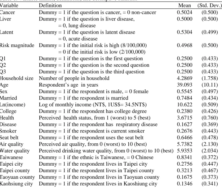
Table 1 reports the definitions of all variables together with the sample means and standard deviations. The sample statistics are consistent with expectations, given the sampling plan. The respondents’ mean age is 39 years, with a range of 16 to 70.
5
quarters of the respondents are married and 55 percent are male. Almost one-quarter have obtained a college degree. The mean income is about US$14,000 per year. Average self-reported health is 3.6 on a five-point scale (where 5 is best). More than one-quarter of the respondents are current smokers, and about one-sixth report they suffer from respiratory illness. About two-thirds routinely use seatbelts when traveling in an automobile.
4. Results
WTP is modeled as a function of health-risk attributes, the respondent’s socio-economic characteristics, and variables characterizing risk attitudes. Regression models are estimated using the maximum-likelihood method under the assumption that WTP is lognormally distributed.6 This section reports estimates of how WTP to reduce health risks depends on the characteristics of those risks as well as on respondents’ personal characteristics.
Effects of Health-Risk Characteristics on WTP
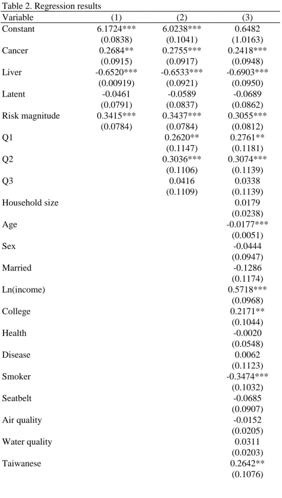
To determine how WTP depends on the characteristics of the health risks, we pool the responses to the four WTP questions and estimate a regression that includes only dummy variables for the various risk characteristics: cancer/non-cancer, latent/acute, liver/lung, and magnitude of risk reduction. The results are shown in column 1 of Table 2.
The estimated coefficients of the cancer and risk-magnitude variables are positive and significant, and that of the liver variable is negative and significant. WTP to reduce the risk of cancer is estimated as 31 percent higher than WTP to reduce the risk of an alternative disease. WTP to reduce the risk of liver disease from water pollution is estimated as 48 percent smaller than WTP to reduce the risk of lung disease from air pollution.
The estimated coefficient of the latent variable is negative, but not significantly different from zero. The point estimate suggests that WTP to reduce current exposure to environmental contaminants that may cause fatal disease is 5 percent smaller if the
6 Using a χ2 test we found that the lognormal model provides a better fit than the Weibull,
exponential, and log-logistic models. The estimated coefficients using alternative distributions have the same signs.
latency period before the disease manifests is 20 years rather than a few months. The insensitivity of WTP to latency suggests that respondents anticipate that their VSL will increase at a rate which nearly offsets their discount rate and conditional survival probability.
The estimated coefficient on risk magnitude allows us to reject the hypothesis that WTP is insensitive to the magnitude of risk reduction, but the magnitude of the
coefficient is much smaller than the value (log(4) ≈1.4) required for estimated WTP to be proportional to magnitude of risk reduction. This result— that WTP is sensitive to risk magnitude, but less than proportionate— is consistent with nearly all previous CV studies of health-risk reduction (Hammitt and Graham, 1999; Krupnick et al., 2002) and may reflect inadequate communication of the quantitative risk reduction to survey respondents (Corso et al., 2001).
To control for question-order effects, we add three question-dummy variables (Q1 – Q3) to the variables describing the risk characteristics. As shown in column 2, estimated WTP is higher in the first and the second valuation questions than in the third and fourth. Payne et al. (2000) also found that question order has a significant effect on CV estimates of WTP. In their study, WTP for the first of five environmental goods was significantly larger than WTP for the remaining goods. Despite the significant effect of question order, controlling for this factor has a negligible effect on the estimated coefficients of the risk characteristics.
In order to identify any differences in the estimated cancer premium or latency effect with disease type or affected organ we added interaction variables to the
specification reported in column 2. Interactions between Cancer and Latent, Cancer and Liver, and Latent and Liver, were entered individually and jointly. None of the
coefficients on these interaction terms were significantly different from zero, and their inclusion had little effect on the magnitude of the other coefficients. (Estimates of these specifications are omitted from the table.)
Effects of Respondent Characteristics on WTP
In column 3 of Table 2, we add respondent characteristics to the risk-characteristic and question-order variables. We omit 96 observations for which personal characteristics
are missing, so the sample size falls from 4,992 (1,248 respondents) to 4,608 (1,152 respondents).
Addition of the respondent characteristics has a minimal effect on the estimated coefficients of the risk-characteristic variables. The cancer premium is estimated as 27 percent and WTP to reduce the risk of liver disease due to water contamination is estimated as 50 percent smaller than WTP to reduce the risk of lung disease due to air pollution. The coefficient on latency remains negative and not significantly different from zero. The implicit discount rate for latency is estimated as 0.3 percent per year, with a 90 percent confidence interval of 1.2 to -0.5 percent per year.7
Socio-economic characteristics of the respondents are significantly associated with estimated WTP. The estimated income elasticity (0.57, standard error = 0.10) is comparable to estimates obtained in other studies of health risk (e.g., Jones-Lee et al., 1985; Mitchell and Carson, 1986; Liu et al., 1997; Corso et al., 2001; Mrozek and Taylor, 2002). Estimated WTP declines with age at a rate of about 1.8 percent per year, and college-educated respondents are estimated to value risk reduction about 24 percent more than respondents with less education. In contrast, WTP is not significantly associated with the number of household members, even though the questions ask about WTP to reduce risk to everyone in the household. In addition, there is no significant association between WTP and either sex or marital status.
Several variables are included as indicators of risk attitudes. Current smokers’ WTP is estimated as 29 percent less than non-smokers’ WTP, consistent with wage-differential studies which also show that smokers value safety less than non-smokers (Hersch and Viscusi, 1990; Hersch and Pickton, 1995; Viscusi and Hersch, 2001). In contrast, use of automobile seatbelts is not significantly related to WTP. Further, WTP is not significantly associated with perceived health status, presence of respiratory disease, or with perceived air and drinking-water quality (after controlling for region).
7
The CV studies reported by Alberini et al. (2002) and Krupnick et al. (2002) included questions about the respondents’ WTP the risk of dying in the next decade and also in the decade following the respondent’s 70th birthday. Comparing these values suggests that respondents discount for latency at annual rates of 4.5 and 8 percent in the US and Canada, respectively (Maureen Cropper, personal communication, July 31, 2002).
WTP is associated with ethnicity and region. Ethnic Taiwanese have a significantly higher WTP than ethnic Chinese, and Taipei city residents have smaller WTP than residents of other areas.
Effect of Latency
Theoretically, the effect of latency on WTP depends on the opportunity cost of funds, the conditional survival probability, and the change in VSL between the current and future times (equation (3)). The change in VSL depends on differences in age, income (related to both life-cycle earnings effects and secular changes in productivity), and other factors. Neglecting these other factors, we can estimate the anticipated change in income that is consistent with the estimated effects of age and latency.
The proportional change in VSL for a latency period of t years can be represented as
(
)
tη t t t t s a g r VSL VSL + + = 1 1 1 0 (4) where VSL0 and VSLt are VSL at the current time and t years in the future, respectively, rand st are the opportunity-cost discount rate and the conditional survival probability (as in
equation (3)), at is a factor describing how VSL depends on age, g is the average annual
income growth rate, and η is the income elasticity.8
From column (3) of Table 3, VSL20/VSL0 is estimated as 0.933, a20 is estimated as e-0.0177 • 20, and η is estimated as
0.572. The conditional survival probability can be estimated from demographic data; we assume a value of 0.9. Substituting these values into equation (4) and rearranging terms yields
(
)
20 20 20 0 20 20 048 . 1 1 1 = = + + η s a VSL VSL r g . (5)Equation (5) implies that the estimated effect of latency is consistent with the estimated age and income effects if respondents’ assume their income will grow at a rate about 5 percent greater than their discount rate over the next 20 years (and the effects of changes
8
in other factors affecting VSL are negligible). Although Taiwan has experienced rapid economic growth in recent years, with real rates of 5 to 6 percent, it seems unlikely that respondents anticipate income growth to average 5 percent greater than interest rates. Hence this result suggests either that respondents anticipate changes in other factors will lead to large increases in VSL, or the responses demonstrate inadequate sensitivity to latency.
Value per Statistical Life
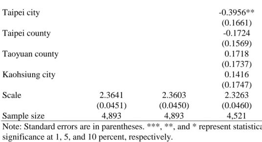
The value per statistical life is calculated by dividing WTP for a reduction in risk by the magnitude of the reduction (equation (2)). Table 3 reports estimates of VSL as a function of disease type, latency, and organ/environmental pathway. These are calculated using the corresponding estimates of WTP from the regression models in Table 2 to predict median WTP at the sample mean of the covariates for each risk reduction, dividing by the risk reduction and average household size (4.3), then averaging over the small and large risk reductions.
Estimated VSL ranges between US$0.5 million and US$1.7 million. These values are substantially smaller than estimates for the US (Viscusi, 1993) and are comparable to previous estimates for Taiwan. Using compensating wage differentials, Liu et al. (1997) estimated a value of approximately US$0.5 million using actuarial risk estimates for 1982–1986, and Liu and Hammitt (1999) estimated VSL in 1995 as US$0.6 million (controlling for injury risk) and US$1.2 million (not controlling for injury risk), using workers’ subjective risk estimates. Using CV, Fu et al. (1999) estimated WTP per statistical case of cancer avoided by reducing pesticide residues on food in Taiwan as US$0.6 – 1.3 million in 1995.
5. Conclusion
Health benefits of environmental regulations are frequently associated with
reduced risks of cancer and of other degenerative and fatal diseases. To date, there is little evidence regarding the extent to which individual WTP to reduce fatal risks differs by characteristics of the risk, including the type of disease or trauma and the latency period between exposure to the hazard and fatal outcome.
In a general-population contingent valuation study in Taiwan, we find that WTP to reduce risks of fatal cancer due to environmental pollution is significantly larger than WTP to reduce risks of an otherwise similar degenerative disease, and that WTP to reduce risks of lung disease due to industrial air pollution is substantially greater than WTP to reduce risks of liver disease due to water pollution. Because these factors are confounded in our study design, we are unable to separately estimate the effects of differences in the affected organ (liver or lung), environmental pathway (drinking and bathing water or air), and payment mechanism (higher water utility bills or higher payments for manufactured goods). Even though we use identical language to describe the symptoms and prognosis of the four diseases, the descriptions are rather brief and respondents may have inferred that cancer is more serious than other disease, or that lung disease is more serious than liver disease.
In contrast, we find that WTP to reduce exposure to environmental pollution is not sensitive to the latency period between exposure and manifestation of disease. The insensitivity of WTP to latency suggests that respondents’ anticipate their VSL will grow over time at a rate about equal to their discount rate. As described in Section 2, the anticipated increase in VSL may reflect changes in age and calendar time. Combining estimates of the effects of age and income growth on VSL (in Section 4) suggests that respondents anticipate a rate of income growth substantially larger than the interest rate, that factors other than income are anticipated to increase VSL, or that responses are inadequately sensitive to the latency period, as they are to the risk increment and to the number of household members.
When evaluating the benefits of environmental regulations, our results suggest that benefits of mortality-risk reduction should not be reduced to account for the latency period between exposure and manifestation of disease. They further suggest the existence of substantial differences in VSL associated with specific diseases. In particular,
reductions in risk of fatal cancer may be more valuable than comparable reductions in other fatal, degenerative disease. Values of risk reduction may also be sensitive to the affected organ and environmental pathway. These results require confirmation and further refinement for use in policy analysis.
Refer ences
Alberini, A., M. Cropper, A. Krupnick, and N.B. Simon, “Does the Value of a Statistical Life Vary with Age and Health Status? Evidence from the United States and Canada,” Discussion Paper 02-19, Resources for the Future, Washington, D.C., 2002.
Arrow, K., R. Solow, P. Portney, E. Leamer, R. Radner, and H. Schuman, “Report of NOAA Panel on Contingent Valuation,” Federal Register 58(10): 4601-4614, 1993.
Buzby, J., R. Ready, and J. Skees, “Contingent Valuation in Food Policy Analysis: A Case Study of a Pesticide-Residue Risk Reduction,” Journal of Agricultural and Applied Economics 27: 613-625, 1995.
Corso, P.S., J.K. Hammitt, and J.D. Graham, “Valuing Mortality-Risk Reduction: Using Visual Aids to Improve the Validity of Contingent Valuation,” Journal of Risk and Uncertainty 23: 165-184, 2001.
Cropper, M.L, and P.R. Portney, “Discounting and the Evaluation of Lifesaving Programs,” Journal of Risk and Uncertainty 3: 369-379, 1990.
Cropper, M.L., and F.G. Sussman, “Valuing Future Risks to Life,” Journal of Environmental Economics and Management 19: 160-174, 1990.
Cropper, M.L., S.K. Ayded, and P.R. Portney, “Preferences for Life Saving Programs: How the Public Discounts Time and Age,” Journal of Risk and Uncertainty 8: 243-265, 1994.
Drèze, J., “L’Utilitè Sociale d’une Vie Humaine,” Revue Française de Recherche Opèrationelle 6: 93-118, 1962.
Environmental Protection Agency, “Protection of Stratospheric Ozone,” Federal Register 52: 47489-47523, December 14, 1987.
Flores, N.E., and R.T. Carson, “The Relationship between the Income Elasticities of Demand and Willingness to Pay,” Journal of Environmental Economics and Management 33: 287-295, 1997.
Fu, T.-T., J.-T. Liu and J.K. Hammitt, “Consumer Willingness to Pay for Low-Pesticide Fresh Produce in Taiwan,” Journal of Agricultural Economics 50: 220-233, 1999. Gerking, S., M. De Haan, and W. Schulze, “The Marginal Value of Job Safety: A
Contingent Valuation Study,” Journal of Risk and Uncertainty 1: 185-199, 1988. Hammitt, J.K.,“Valuing Mortality Risk: Theory and Practice,” Environmental Science
and Technology 34(8): 1396-1400, 2000a.
Hammitt, J.K.,“Evaluating Contingent Valuation of Environmental Health Risks: The Proportionality Test,” Association of Environmental and Resource Economists Newsletter 20(1): 14-19, May 2000. Reprinted in Stated Preference: What Do We
Know? Where Do We Go? (Proceedings). Report number EE-0436, U.S. Environmental Protection Agency, October 2000b.
Hammitt, J.K., and J.D. Graham, “Willingness to Pay for Health Protection: Inadequate Sensitivity to Probability?” Journal of Risk and Uncertainty 18: 33-62, 1999. Hanemann, W.M., J. Loomis, and B. Kanninen, “Statistical Efficiency of
Double-Bounded Dichotomous Choice Contingent Valuation,” American Journal of Agricultural Economics 73: 1255-1261, 1991.
Hersch, J., and T.S. Pickton, “Risk-Taking Activities and Heterogeneity of Job-Risk Tradeoffs,” Journal of Risk and Uncertainty 11: 205-217, 1995.
Hersch, J., and W.K. Viscusi, “Cigarette Smokers, Seatbelt Use, and Differences in Wage-Risk Tradeoffs,” Journal of Human Resources 25: 202-227, 1990. Horowitz, J., and R.T. Carson, “Discounting Statistical Lives,” Journal of Risk and
Uncertainty 3: 403-413, 1990.
Johannesson, M., P-O Johansson, and K-G Lofgren., “On the Value of Changes in Life Expectancy: Blips Versus Parametric Changes,” Journal of Risk and Uncertainty 15: 221-239, 1997.
Jones-Lee, M., “The Value of Changes in the Probability of Death or Injury,” Journal of Political Economy 82: 835-849, 1974.
Jones-Lee, M.W., M. Hammerton, and P.R. Philips, “The Value of Safety: Results of a National Sample Survey,” The Economic Journal 95: 49-72, 1985.
Kimball, M.S., “Precautionary Saving in the Small and in the Large,” Econometrica 58: 53-73, 1990.
Krupnick, A., A. Alberini, M. Cropper, N. Simon, B. O’Brien, R. Goeree, and M. Heintzelman, “Age, Health and the Willingness to Pay for Mortality Risk Reductions: A Contingent Valuation Survey of Ontario Residents,” Journal of Risk and Uncertainty 24: 161-186, 2002.
Lee, S.J., P.J. Neumann, W.H. Churchill, M.E. Cannon, M.C. Weinstein, and M. Johannesson, “Patients’ Willingness to Pay for Autologous Blood Donation,” Health Policy 40: 1-12, 1997.
Liu, J.-T., and J.K. Hammitt, “Perceived Risk and Value of Workplace Safety in a Developing Country,” Journal of Risk Research 2: 263-275, 1999.
Liu, J.-T., J.K. Hammitt, and J.-L. Liu, “Estimated Hedonic Wage Function and Value of Life in a Developing Country,” Economics Letters 57: 353-358, 1997.
Magat, W.A., W.K. Viscusi, and J. Huber, “A Reference Lottery Metric for Valuing Health,” Management Science 42: 1118-1130, 1996.
McDaniels, T.L., M.S. Kamlet, and G.W. Fischer, “Risk Perception and the Value of Safety,” Risk Analysis 12: 495-503, 1992.
Mendeloff, J.M., and R.M. Kaplan, “Are Large Differences in ‘Lifesaving’ Costs Justified? A Psychometric Study of the Relative Value Placed on Preventing Deaths,” Risk Analysis 9: 349-363, 1989.
Mitchell, R.C., and R.T. Carson, “Valuing Drinking Water Risk Reductions Using the Contingent Valuation Method: A Methodological Study of Risks from THM and Giardia,” Resources for the Future, Washington, D.C., 1986.
Moore, M.J., and W.K. Viscusi, “Discounting Environmental Health Risks: New Evidence and Policy Implications,” Journal of Environmental Economics and Management 18: S51-S62, 1990.
Mrozek, J.R., and L.O. Taylor, “What Determines the Value of Life? A Meta Analysis,” Journal of Policy Analysis and Management 21: 253-270, 2002.
National Center for Health Statistics, Health, United States, US Department of Health and Human Services, Hyattsville, Maryland, 1998.
Ng, Y.-K., “The Older the More Valuable: Divergence Between Utility and Dollar Values of Life as One Ages,” Journal of Economics 55: 1-16, 1992.
Payne, J.W., D.A. Schkade, W.H. Desvousges, and C. Aultman, “Valuation of Multiple Environmental Programs,” Journal of Risk and Uncertainty 21: 95-115, 2000. Revesz, R.L., “Environmental Regulation, Cost-Benefit Analysis, and the Discounting of
Human Lives,” Columbia Law Review 99: 941-1017, 1999.
Rosen, S., “The Value of Changes in Life Expectancy,” Journal of Risk and Uncertainty 1: 285-304, 1988.
Savage, I., “An Empirical Investigation into the Effect of Psychological Perceptions on the Willingness-to-Pay to Reduce Risk,” Journal of Risk and Uncertainty 6: 75-90, 1993.
Schelling, T.C., “The Life You Save May Be Your Own,” in S.B. Chase (ed.), Problems in Public Expenditure Analysis, Brookings, Washington, D.C., 1968.
Shepard, D.S., and R.J. Zeckhauser, “Survival versus Consumption,” Management Science 30: 423-439, 1984.
Smith, V.K., H. Kim, and D.H. Taylor, “Do the ‘Near’ Elderly Value Mortality Risks Differently?” presented at the Workshop on Assessing and Managing
Environmental and Public Health Risks, Association of Environmental and Resource Economists, Bar Harbor, Maine, June 2001.
Subramanian, U., and M. Cropper, “Public Choices Between Life Saving Programs: The Tradeoff Between Qualitative Factors and Lives Saved,” Journal of Risk and Uncertainty 21: 117-149, 2000.
Sunstein, C.R., “Bad Deaths,” Journal of Risk and Uncertainty 14: 259-282, 1997. Viscusi, W.K., “The Value of Risks to Life and Health,” Journal of Economic Literature
Viscusi, W.K., and J. Hersch, “Cigarette Smokers as Job Risk Takers,” Review of Economics and Statistics 83: 269-280, 2001.
Weinstein, M.C., D.S. Shepard, and J.S. Pliskin, “The Economic Value of Changing Mortality Probabilities: A Decision-Theoretic Approach,” Quarterly Journal of Economics 94: 373-396, 1980.
Table 1. Variable names, definitions, and descriptive statistics
Variable Definition Mean (Std. Dev.)
Cancer Dummy = 1 if the question is cancer, = 0 non-cancer 0.5024 (0.500) Liver Dummy = 1 if the question is liver disease,
= 0, lung disease
0.5000 (0.500) Latent Dummy = 1 if the question is latent disease
= 0, acute disease
0.5304 (0.499) Risk magnitude Dummy = 1 if the initial risk is high (8/100,000)
= 0 if the initial risk is low (2/100,000)
0.4968 (0.500) Q1 Dummy = 1 if the question is the first question 0.2500 (0.433) Q2 Dummy = 1 if the question is the second question 0.2500 (0.433) Q3 Dummy = 1 if the question is the third question 0.2500 (0.433)
Household size Number of people in household 4.2869 (1.758)
Age Respondent’s age in years 39.093 (10.11)
Sex Dummy = 1 if the respondent is male, = 0 female 0.5545 (0.497) Married Dummy = 1 if the respondent is married 0.7484 (0.434) Ln(income) Log of monthly income (NT$, 1US$= 34.5NT$) 10.622 (0.509) College Dummy = 1 if the respondent has college degree 0.2380 (0.426) Health Perceived health status, from 1 (worst) to 5 (best) 3.6715 (0.760) Disease Dummy = 1 if the respondent has respiratory disease 0.1627 (0.369) Smoker Dummy = 1 if the respondent is current smoker 0.2676 (0.443) Seat belt Dummy = 1 if the respondent uses the seat belt 0.6466 (0.478) Air quality Perceived air quality, from 0 (worst) to 10 (best) 5.7382 (2.130) Water quality Perceived drinking water quality, from 0 (worst) to 10 (best) 5.9353 (2.034) Taiwanese Dummy = 1 if the ethnic is Taiwanese, = 0 Chinese 0.8341 (0.372) Taipei city Dummy = 1 if the respondent lives in Taipei city 0.2756 (0.447) Taipei county Dummy = 1 if the respondent lives in Taipei county 0.3213 (0.467) Taoyuan county Dummy = 1 if the respondent lives in Taoyuan county 0.1675 (0.373) Kaohsiung city Dummy = 1 if the respondent lives in Kaoshiung city 0.1346 (0.341)
Table 2. Regression results Variable (1) (2) (3) Constant 6.1724*** 6.0238*** 0.6482 (0.0838) (0.1041) (1.0163) Cancer 0.2684** 0.2755*** 0.2418*** (0.0915) (0.0917) (0.0948) Liver -0.6520*** -0.6533*** -0.6903*** (0.00919) (0.0921) (0.0950) Latent -0.0461 -0.0589 -0.0689 (0.0791) (0.0837) (0.0862) Risk magnitude 0.3415*** 0.3437*** 0.3055*** (0.0784) (0.0784) (0.0812) Q1 0.2620** 0.2761** (0.1147) (0.1181) Q2 0.3036*** 0.3074*** (0.1106) (0.1139) Q3 0.0416 0.0338 (0.1109) (0.1139) Household size 0.0179 (0.0238) Age -0.0177*** (0.0051) Sex -0.0444 (0.0947) Married -0.1286 (0.1174) Ln(income) 0.5718*** (0.0968) College 0.2171** (0.1044) Health -0.0020 (0.0548) Disease 0.0062 (0.1123) Smoker -0.3474*** (0.1032) Seatbelt -0.0685 (0.0907) Air quality -0.0152 (0.0205) Water quality 0.0311 (0.0203) Taiwanese 0.2642** (0.1076)
Taipei city -0.3956** (0.1661) Taipei county -0.1724 (0.1569) Taoyuan county 0.1718 (0.1737) Kaohsiung city 0.1416 (0.1747) Scale 2.3641 2.3603 2.3263 (0.0451) (0.0450) (0.0460) Sample size 4,893 4,893 4,521
Note: Standard errors are in parentheses. ***, **, and * represent statistical significance at 1, 5, and 10 percent, respectively.
Table 3. Estimated value per statistical life (million US$)
Disease type Latency Organ/pathway (1) (2) (3)
Cancer Latent Lung 1.6 1.6 1.3
Cancer Acute Lung 1.7 1.7 1.4
Non-cancer Latent Lung 1.3 1.2 1.0
Non-cancer Acute Lung 1.3 1.3 1.1
Cancer Latent Liver 0.9 0.9 0.6
Cancer Acute Liver 0.9 0.9 0.7
Non-cancer Latent Liver 0.7 0.6 0.5
Non-cancer Acute Liver 0.7 0.7 0.5
Note: Estimates correspond to models in corresponding column of Table 2.
Appendix: Sur vey Questions 1. Liver disease / water pathway
As you know, the drinking water that is piped to your home is treated to remove microbial and chemical contaminants. However, there is always a risk that some contaminants may be present in the water.
Consider what you would do if you learned that there is a contaminant in the water supplied to your home that may cause [liver cancer / liver failure]. You and other people in your household can be exposed to the contaminant by drinking the water, and also by using it for bathing. The chance that you or someone in your household will be exposed to enough of this contaminant to cause [liver cancer / liver failure] is [2 / 8] chances in 100,000 per year.
Insert [Acute] or [Latent] description:
[Acute] The type of [liver cancer / liver failure] caused by this contaminant is always fatal. If someone in your household is exposed to enough of the contaminant to develop [liver cancer / liver failure], they will develop symptoms within a few months, and will live only about 2 to 3 years longer.
[Latent] The type of [liver cancer / liver failure] caused by this contaminant is always fatal, but it takes a long time to develop. If someone in your household is exposed to enough of the contaminant to develop [liver cancer / liver failure], they will not know it until they begin to experience symptoms about 20 years later. After developing these symptoms, they will live only about 2 to 3 years longer.
If someone in your household develops [liver cancer / liver failure], the symptoms will be mild at first. Eventually, they will become so weak that they will have to stay in bed or a wheel chair most of the time. They will not be able to take care of themselves. Once this occurs, they will die within one to two months.
The water-treatment plant can install additional treatment equipment to reduce the chance that the contaminant will be in your water. The treatment equipment is expensive, and the people who manage the plant are not sure if it is worth the cost. If the treatment
equipment is installed, it will reduce the chance that someone in your household will be exposed to enough of the contaminant to develop [liver cancer / liver failure] from [2 / 8] chances in 100,000 per year to almost zero— to only 1 chance in 10 million per year. If the plant installs the equipment, it will need to recover the cost by increasing the amount that consumers pay for their water. If the additional cost to your household would be NT$ [50, 100, 200, 300, 500] per month, would you want the plant to install the
treatment equipment to reduce the chance that you or someone else in your household would develop [liver cancer / liver failure]?
2. Lung disease / air pathway
Air pollution that is released from factories may cause [lung cancer / bronchitis]. Consider what you would do if you learned that the chance that someone in your
household will be exposed to enough of this pollution to cause [lung cancer / bronchitis] is [2 / 8] chances in 100,000 per year.
Insert [Acute] or [Latent] description:
[Acute] The type of [lung cancer / bronchitis] caused by this pollution is always fatal. If someone in your household is exposed to enough of the pollution to develop [lung cancer / bronchitis], they will develop symptoms within a few months, and will live only about 2 to 3 years longer.
[Latent] The type of [lung cancer / bronchitis] caused by this pollution is always fatal, but it takes a long time to develop. If someone in your household is exposed to enough of the pollution to develop [lung cancer / bronchitis], they will not know it until they begin to experience symptoms about 20 years later. After developing these symptoms, they will live only about 2 to 3 years longer.
If someone in your household develops [lung cancer / bronchitis], the symptoms will be mild at first. Eventually, they will become so weak that they will have to stay in bed or a wheel chair most of the time. They will not be able to take care of themselves. Once this occurs, they will die within one to two months.
The government can require factories to install additional air-pollution-control equipment to reduce the amount pollution coming out of the factory. The equipment will reduce the chance that someone in your household will be exposed to enough of the pollution to develop [lung cancer / bronchitis] from [2 / 8] chances in 100,000 per year to almost zero— to only 1 chance in 10 million per year.
If the government requires the factories to install this pollution-control equipment, it will increase the cost of many of the goods you buy. This would increase your cost of living. If the additional cost to your household would be NT$ [50, 100, 200, 300, 500] per month, would you want the factories to install the pollution-control equipment to reduce the chance that you or someone else in your household would develop [lung cancer / bronchitis]?
Table A-1. Survey design
Sub-sample A1 A2
Question 1 low risk, latent, liver cancer high risk, acute, liver cancer Question 2 low risk, acute, liver cancer high risk, latent, liver cancer Question 3 low risk, latent, bronchitis high risk, latent, bronchitis Question 4 low risk, acute, bronchitis high risk, acute, bronchitis
Sub-sample A3 A4
Question 1 low risk, latent, liver failure high risk, latent, liver failure Question 2 low risk, acute, liver failure high risk, acute, liver failure Question 3 low risk, acute, bronchitis high risk, latent, bronchitis Question 4 low risk, latent, bronchitis high risk, acute, bronchitis
Sub-sample B1 B2
Question 1 low risk, latent, lung cancer high risk, acute, lung cancer Question 2 low risk, acute, lung cancer high risk, latent, lung cancer Question 3 low risk, acute, liver cancer high risk, latent, liver cancer Question 4 low risk, latent, liver cancer high risk, acute, liver cancer
Sub-sample B3 B4
Question 1 low risk, latent, bronchitis high risk, latent, bronchitis Question 2 low risk, acute, bronchitis high risk, acute, bronchitis Question 3 low risk, acute, liver cancer high risk, latent, liver cancer Question 4 low risk, latent, liver cancer high risk, acute, liver cancer Note: Describes the risk characteristics of the four questions asked to each of eight sub-samples of respondents.