高行動性OFDM系統之聯合時域與頻遇通道估計

國 立 交 通 大 學

電信工程學系碩士班

碩士論文

高行動性

OFDM 系統之聯合時域與頻域通道估

計

Joint Time and Frequency Domain Channel Estimation

for High-Mobility OFDM Systems

研 究 生：高祥倫

中華民國九十六年七月

高行動性

OFDM 系統之聯合時域與頻域通道估計

Joint Time and Frequency Domain Channel Estimation for

High-Mobility OFDM Systems

研 究 生：高祥倫 Student：Shiang-Lun Kao

指導教授：吳文榕 博士 Advisor：Dr. Wen-Rong Wu

國 立 交 通 大 學

電信工程學系碩士班

碩 士 論 文

A Thesis

Submitted to Department of Communication Engineering

College of Electrical and Computer Engineering

National Chiao-Tung University

in Partial Fulfillment of the Requirements

for the Degree of

Master of Science

In

Communication Engineering

July 2007

Hsinchu, Taiwan, Republic of China

高行動性

OFDM 系統之聯合時域與頻域

通道估計

研究生：高祥倫 指導教授：吳文榕 教授

國立交通大學電信工程學系碩士班

摘要

在時變的 OFDM 系統下，通道估計通常倚賴著響導訊號。然而，嚮導訊號的 數目是有限的。因此在接收機設計上，通道估計即為一項關鍵性的工作。在本篇 論文中，我們首先針對 IEEE802.16e 系統提出一個二維滑行視窗通道估測器。在 性能上不僅勝過傳統的方法，並且能有低複雜度。為了更近一步的提升系統效 能，我們提出了一個結合了時域與頻域的高效能最小平方估測器。主要的概念是 利用頻域上通道估計的結果，來求得時域上通道響應的位置。接著利用最小平方 演算法來估計這些位置上的通道響應。並且利用遞迴演算法，我們能進一步得到 更精準的通道估計。在運算複雜度上，也比傳統時域上的最小平方估測器來的小。

Joint Time and Frequency Domain Channel Estimation for

High-Mobility OFDM Systems

Student:

Shiang-Lun

Kao

Advisor: Dr. Wen-Rong Wu

Department of Communication Engineering

National Chiao-Tung University

Abstract

In time-variant OFDM systems, channel estimation usually relies on pilot subcarriers. However, the number of pilot subcarriers is usually limited. Channel estimation is then a critical task for receiver design. In this thesis, we first propose a two-dimension slide-window channel estimator for IEEE802.16e systems. The estimator can outperform conventional approaches and requires low-complexity. To further improve the performance, we then propose a high-performance least-squares (LS) channel estimator, joint operated in the time and frequency domains. The main idea is use the channel response, estimated in the frequency domain, to locate significant time-domain channel taps, and then use the LS method to estimate the responses in those taps. With an iterative algorithm, we can then obtain accurate channel estimate with computational complexity much lower than the conventional time domain LS estimator.

致謝

本篇論文得以順利完成，第一個要特別感謝我的指導教授 吳文

榕博士，不管在課業學習、論文研究上，都給了我很多的指教以及相

當程度的自由，甚至教導我在做人處事及對面問題應該有的態度。

另外，我要感謝許兆元學長、楊華龍學長、李俊芳學長、謝弘道

學長等在研究上不吝指導，也要感謝丁偉家同學、吳俊穎同學、林育

丞同學，與我在各種課業以及論文研究上頻繁的討論。寬頻傳輸與訊

號處理實驗室是個很好的大家庭，能夠在此與各位學長姐、同學、學

弟妹一起研究、生活，讓我備感溫馨與榮幸。我還要感謝我的大學同

學 蔡依修、張書維、吳政鴻，在我生活、課業或感情遇到問題時，

給了我許多的建議。

最後我要感謝我的家人與女朋友，在我念研究所的期間，給予我

精神上的鼓勵與支持，使得我可以順利地完成碩士學位。

Contents

中文摘要 I Abstract II 致謝 III Contents IV List of Tables V List of Figures VI Chapter 1 Introduction 1

Chapter 2 OFDM System and Channel Estimation 3

2.1 Introduction to OFDM System 3

2.1.1 Basic Principle of OFDM System 5

2.1.2 Cyclic Prefix 8

2.1.3 Discrete-Time Equivalent System Model 9

2.2 Introduction to IEEE 802.16e 11

2.2.1 Generic OFDMA Symbol Description 12

2.2.1.1 Time Domain Description 12

2.2.1.2 Frequency Domain Description 12

2.2.1.3 Primitive Parameters 12

2.2.1.4 Derived Parameters 13

2.2.2 DL Preamble Structure and Modulation 13

2.2.3 DL Carrier Allocation 15

2.2.3.1 DL PUSC 15

2.2.3.2 DL FUSC 17

2.2.4 DL Carrier Modulation 18

2.2.4.2 DL Data Modulation 19

2.3 Conventional Time-Invariant Channel Estimator 20

2.3.1 LS Channel Estimator 20

2.3.2 MMSE Channel Estimator 22

2.3.3 Frequency Domain Interpolation Methods 23

Chapter 3 Proposed Channel Estimator 29

3.1 Sliding-Windowed LAQ Channel Estimator 31

3.2 Low-Complexity Time Domain Channel Estimator 32

3.3 Channel Tap Search Algorithm 34

3.3.1 Preliminary Channel Estimation with Preamble 34

3.3.2 Preliminary Channel Estimation with Pilots 35

3.3.3 Channel Tap Search Method 36

3.4 Joint Time and Freq Domain Channel Estimator 38

3.5 Time-Variant Channel Estimation 41

Chapter 4 Simulation Results 44

4.1 Channel Model 45

4.2 Sliding-Windowed LAQ Results 46

4.3 Low-Complexity Time Domain Channel Estimation Results 49

4.4 Joint Time and Freq Domain Channel Estimation Results 51

4.5 Time-Variant Channel Estimation Results 53

Chapter 5 Conclusion and Future Works 57

List of Tables

List of Figures

Figure 2-1 Block diagram of an OFDM system 5

Figure 2-2 Subdivision of the bandwidth 5

Figure 2-3 Continuous-time OFDM baseband modulator 6

Figure 2-4 Continuous-time OFDM baseband demodulator 7

Figure 2-5 Overlapping and orthogonal transmission spectrums 7

Figure 2-6 Cyclic prefix 9

Figure 2-7 Equivalent discrete-time model 10

Figure 2-8 Preamble for each segment 14

Figure 2-9 Cluster structure 15

Figure 2-10 Modulation constellations 19

Figure 2-11 A polynomial interpolator 25

Figure 2-12 Channel estimation with 2-cluster quadratic interpolator 26

Figure 2-13 Channel estimation with LAQ interpolator 28

Figure 3-1 Discontinuousness in boundary areas 31

Figure 3-2 Slideing-window LAQ method 32

Figure 3-3 Equation for OFDM receive signal in frequency domain 34

Figure 3-4 Preliminary channel estimation (with preamble) 35

Figure 3-5 Result of the preliminary channel estimation 36

Figure 3-6 Channel tap searching method (threshold dependent) 36

Figure 3-7 Channel tap searching method by first-order differentiation 37

Figure 3-8 Iterative channel tap searching method 38

Figure 3-9 Proposed channel estimation flowchart 39

Figure 3-12 Time-variant channel estimation 42

Figure 4-1 Simulation platform 44

Figure 4-2 Channel generated by SCM model 46

Figure 4-3 BER comparison for various interpolation methods 46

Figure 4-4 BER comparison for various channel estimation methods (55T_S< delay spread < 85T_S) 47

Figure 4-5 Estimated frequency response for various estimation methods 48

Figure 4-6 BER comparison for various channel estimation methods (delay spread > 85T_S) 48

Figure 4-7 BER performance comparison for various estimation methods (delay spread > 85T_S) 49

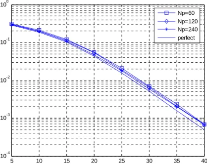
Figure 4-8 BER performance vs. number of used pilot signals (55T_S< delay spread < 85T_S) 50

Figure 4-9 BER performance vs. number of used pilot signals (delay spread > 85T_S) 50

Figure 4-10 Preliminary channel estimation result with pilots 51

Figure 4-11 Iterative location of channel taps 52

Figure 4-12 BER performance for proposed channel estimator (55T_S< delay spread < 85T_S) 52

Figure 4-13 BER performance for different mobile speed (55T_S< delay spread < 85T_S) 54

Figure 4-14 BER performance for different mobile speed (delay spread > 85T_S) 54

Figure 4-15 Time variation of a channel tap for mobile speed = 50km/hr 55 Figure 4-16 Time variation of a channel tap for mobile speed = 100km/hr 55 Figure 4-17 Time variation of a channel tap for mobile speed = 200km/hr 56 Figure 4-18 BER performance for ICI cancellation by MMSE equalizer 56

Chapter 1

Introduction

In recent years, the demand for high data rate services increases rapidly, e.g., high quality video and audio data. Thus, the next generation communication systems are expected to use transmission schemes with high spectrum efficiency. Multicarrier techniques, usually referred to as Orthogonal Frequency Division Multiplexing (OFDM) modulation, are well-known for its efficient spectrum usage. Despite its spectrum efficiency, this technique is often applied in wireless communication systems due to its robustness against multipath channel fading. Due to these properties, it has been used in many commercial systems such as digital audio broadcasting (DAB), digital video broadcasting Terrestrial (DVB-T)s, and wireless Local Area Network (LAN) systems. It has also been proposed for wireless broadband access standards such as the IEEE 802.16 (WiMAX) and as the core technique for the fourth-generation (4G) wireless mobile communication.

For high data rate transmission, wireless channels may be fading in both time and frequency, rapidly. Due to the time-variant property, pilots are added to aid channel estimation. However, the inclusion of pilot transmission will reduce the data rate, adversely affect the spectrum efficiency. As a result, the number of pilots is usually very limited. How to conduct time-variant estimation with limited pilots becomes a critical task for receiver design.

In OFDM systems, the receive signal appears as a multiplication of the channel response and the transmit data symbol in the frequency domain. It is simple to equalize signals with a one tap frequency domain equalizer (FEQ). As a result, channel estimation is often conducted in the frequency domain for OFDM systems. As mentioned, pilots are limited and channel estimation usually involves interpolation. The main problem of the frequency domain approach is that when the delay spread of the channel is large, the coherent bandwidth becomes small and accurate interpolation becomes difficult. Channel estimation can be conducted in the time domain with well-known least-squares (LS) and minimum-mean-square-error (MMSE) methods [1] [2]. Although good performance can be obtained, the required computational complexity is very high in general. Besides, the MMSE channel estimator needs to know the channel statistical characteristics, usually not available in practice. In this thesis, we will develop a high-performance yet low-complexity LS channel estimator to overcome the problem. The proposed method estimates the channel in the time as well as in the frequency domain. With an iterative algorithm, we can obtain accurate channel estimate with the computational complexity much lower than the conventional LS algorithm.

This thesis is organized as follows. First, in Chapter 2, we give some OFDM basics and introductions to the IEEE 802.16e OFDMA downlink standard. Then, various channel estimation techniques are reviewed. In Chapter 3, we described two proposed channel estimators, one is an enhanced interpolation method for channel estimation in the frequency domain, and the other is a joint time and frequency domain channel estimator. In Chapter 4, we show simulation results, demonstrating the effectiveness of proposed algorithms. Then we draw conclusions and outline

Chapter 2

OFDM System and Channel Estimation

2.1 Introduction to OFDM System

The basic concept of Orthogonal Frequency Division Multiplexing (OFDM) technique is to increase the symbol duration by splitting the high data-rate stream into lower data-rate streams, and equivalent to divide available wideband channel into narrowband subchannels. Each data stream is transmitted with a subcarrier in a subchannel. Moreover, these subcarriers are designed orthogonal to allow spectrum overlapping. As a result, the scheme can achieve high spectral efficiency. Since the bandwidth of each subchannel is narrow, each transmitted signal in the subchannel experiences flat channel fading. Thus, channel equalization is simplified to a one-tap frequency domain equalizer. Other requirements are summarized as follows [3] [4] [5]:

1. DFT and IDFT are used for conducting signal modulation and demodulation on orthogonal subcarriers. This signal processing function replaces the conventional bank of I/Q modulators and demodulators. Usually, the number of subcarrier is set as power of two. As a result, the DFT/IDFT operations can be efficiently implemented by the FFT/IFFT algorithm.

front of an OFDM symbol, and must be larger than the maximum channel delay spread to avoid ISI effect. Due to the CP, the transmitted signal becomes partially periodic, and the effect of the linear convolution with a multipath channel can be translated to a circular convolution at the receiver. Thanks to circular convolution, the channel effect is simplified to a point-to- point multiplication of the data constellations and channel frequency response. Thus, only a one-tap frequency domain equalizer is required.

3. Error control coding is often be used to enhance the reliability of signal detection. Usually, interleaving is along with coding to achieve the time diversity. Spreading coded bits over the transmission band can achieve frequency diversity (within the frequency selective channel).

4. Synchronization in time and frequency are required. The mission is to identify the start of the OFDM symbol and to align local oscillator frequency with transmission side.

Figure 2-1 shows the block diagram of an OFDM system, where the upper path is the transmitter chain, and the lower path the receiver chain. First, input data are encoded by the channel encoder. The encoded bits are then interleaved and mapped onto QAM constellations. After that, a block of input QAM symbols are modulated onto subcarriers by IFFT operation, and then CP is added to form an OFDM symbol. Finally, the baseband OFDM transmitted signal is passed to the analog-to-digital (A/D) converter and the RF circuit for transmission. In the receiver, time and frequency synchronization, and channel estimation are conducted first, then the reverse operation of the transmitter.

Figure 2-1 Block diagram of OFDM system

2.1.1 Basic Principle of OFDM System

For multicarrier modulation, the available bandwidth W is divided into a number of subbands, each of width Δ =f W N/ . Carriers in those subbands are

commonly called subcarriers. The subdivision of the bandwidth is illustrated in Figure 2-2, where arrows represent the different subcarriers. Instead of transmitting the data symbols in a serial way, at a baud rate R, a multicarrier transmitter partitions the

data stream into blocks of data symbols that are transmitted in parallel by modulating carriers. The symbol duration for a multicarrier scheme is then

. N N / S T =N R

Figure 2-2 Subdivision of the bandwidth

A typical continuous-time OFDM baseband modulator is shown in Figure 2-3. The input data steam is split into parallel streams which modulate different subcarriers and then transmitted simultaneously.

Figure 2-3 Continuous-time OFDM baseband modulator The k-th modulating subcarrier can be represented as

2 ( )

,0

( )

0,

S g j k t T T k

t

e

otherwise

π

φ

⎧⎪⎨ − ⎪⎩

≤ ≤

t T

=

(2.1)

where T is the symbol duration excluding CP, T_g is the length of CP and is the total symbol duration, i.e.

S

T

g S

T = +T T . Let be defined as the transmitted

data, which is a complex number from a set of signal constellation points, at the -th subcarrier for the -th symbol. The modulated baseband signal of the -th OFDM symbol is then ( ) i X k k i i 1 0

( )

N

( ) (

)

i i S k k

x t

X k

φ

t iT

− =

=

∑

−

(2.2) When an infinite sequence of OFDM symbols is transmitted, the output transmitter can be represented as 1 0 ( ) ( ) ( )

( )

i N i S k i i k x t X k t

x t

φ

∞ ∞ − =−∞ =−∞ = =

=

∑

∑ ∑

−iT (2.3) The received signal y t( ) can be expressed as

y t

( )

∞ h t( , ) (

τ

x t

τ τ

)d w t( )

−∞ − +

=

_∫

(2.4) where h t( , )

τ

denotes the time-variant channel impulse response at time , and

additive white complex Gaussian noise.

t

( )

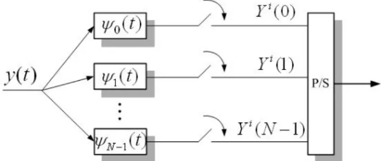
Figure 2-4 Continuous-time OFDM baseband demodulator

A typical continuous-time OFDM baseband demodulator is shown in Figure 2-4, in which

ψ

k( )t denotes the matched filter for the k-th subcarrier.

2 1 ,0 0,

( )

j kt S k e t T otherwise

t

π T

ψ

⎧⎪⎨ ⎪⎩ ≤ ≤

=

(2.5)

In the figure, denotes the demodulated signal at -th subcarrier for the -th symbol.

( )

i

k

Y

k i

Figure 2-5 shows the overlapping and orthogonal transmission spectrums of the modulated signals. Because of the sinc shape of the spectrums, they overlap with each other expect for the frequency points where subcarriers allocate. The subcarrier spacing between two neighbor subcarrier is 1

T . As we can see, OFDM systems have

high bandwidth efficiency.

Figure 2-5 Overlapping and orthogonal transmission spectrums

The symbol duration can be made long compared to the maximum channel delay spread, TS >>

τ

max , by choosing N sufficiently high. At the same time, the bandwidth of the subbands can be made small comparing the coherence bandwidth of

the channel ( ). Signals in subbands then experience flat fading, which reduces equalization to a single complex multiplication per carrier. Since the channel is time-variant, the performance is degraded when the symbol duration is large. If the coherent time of the channel is small compared to , the channel frequency response will change significantly during the transmission of one symbol, inducing Inter-Carrier Interference (ICI) effect. As a result, the coherent time of the channel defines an upper bound for the number of subcarrier. Together with the condition for flat fading, a reasonable range for is given by

/ C W N B >> C T TS N _C C W N RT B << << (2.6)

2.1.2 Cyclic Prefix

A CP is a copy of some tail part of the OFDM symbol, shown in Figure 2-6. The CP should be larger than the maximum channel delay spread to avoid ISI effect. Thus, the signals and their own delayed-version signals resulting from the multipath channel are still periodic within the DFT interval. The orthogonality between subcarriers can be maintained after modulated signals pass through the channel. So, the introduction of CP can overcome the ISI and ICI effects. Besides, it also converts the linear convolution (of the channel impulse response and the transmit signal) into a cyclic one. However, the transmitted energy increases with the length of the CP. The SNR loss is given by 10log (1₁₀ g) loss S T T

SNR

= − − (2.7)

Figure 2-6 Cyclic prefix

2.1.3 Discrete-Time Equivalent System Model

In section 2.1.1, the continuous-time OFDM baseband modulator and demodulator are introduced. The modulated baseband signal for the OFDM symbol is

2 1 0 ,0

1

( )

N jTkt k k t T

x t

X e

T

π − = ≤ ≤

=

∑

(2.8) where X_k is the transmitted data symbols and N is the number of subcarriers.

Consider a discrete-time system. Let t=nT_d, in which d

T N

T = is the sampling

period. Equation (2.8) can be rewritten as 2 1 0 1 ( ) ,0 1

( )

d j kn N N k t nT k x t X e n N N

x n

π − = = = ≤ ≤ −

=

∑

(2.9)

Using the same way, we have the received signal as 2 1 0 1 [ ] j kn N N k n x n e N

Y

π − − = =

∑

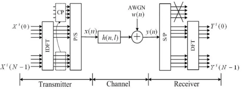
(2.10) So, the modulation in the transmitter and the demodulation in the receiver can be implemented by IDFT and DFT, respectively. The well-known fast DFT/IDFT algorithm, FFT/IFFT, can then be applied for complexity reduction. Figure 2-7 shows the discrete-time equivalent model.

Figure 2-7 Equivalent discrete-time model

The modulation operation can then be described as follows. In the transmitter, the data stream is grouped in blocks of data symbols, called OFDM symbols. Then an IDFT is performed for each data symbol block, and a CP of length

N

g

T is

added. Passing the resultant signal through a time-variant multipath channel, we have the received signal as

(2.11) 1 0 ( , ) ( ) ( )

( )

L _N l h n l x n l w n

y n

− = − +

=

∑

where h n l( , ) is the -th channel path at time instant , l n L is the number of

channel taps,

( )

_N represents a cyclic shift in the base of N, and is sampled additive white complex Gaussian noise with variance

( )

w n 2

σ

. In the receiver, the incoming sequence is split into blocks and the CP associated with each block is removed. Finally, a DFT is performed for each symbol to recover the original data symbols.

As mentioned, carriers in subbands experience flat fading, which reduces equalization to a single complex multiplication per carrier. A matrix equivalent model can be used to obtain a more compact form. For a single OFDM symbol, the received signal can be represented as

(2.12) (0) (0) 0 0 (0) (1) 0 (1) (1) 0 ( 1) 0 0 ( 1) ( 1) Y H X Y H Y N H N X N ⎡ ⎤ ⎡ ⎤ ⎡ ⎢ ⎥ ⎢ ⎥ ⎢ ⎢ ⎥ ⎢₌ ⎥ ⎢ ⎢ ⎥ ⎢ ⎥ ⎢ ⎢ ₋ ⎥ ⎢ ₋ ⎥ ⎢ ⎣ ⎦ ⎣ ⎦ ⎣ L M M M O M L X ⎤ ⎥ ⎥ ⎥ ⎥ − ⎦

where are the transmitted data symbols, and are the channel frequency response.

[ (0), (1), , ( 1)]T

X X _L X N−

{[ (0), (1), , ( 1)]}

diag H H L H N−

2.2 Introduction to IEEE 802.16e

The IEEE standard 802.16 specifies the Wireless Metropolitan Area Network (WMAN). There are four PHY specifications given in 802.16 such as, Single Carrier (SC), Single Carrier a (SCa), Orthogonal Frequency Division Multiplexing (OFDM), and Orthogonal Frequency Division Multiplexing Access (OFDMA) [6] [7]. Each appropriates to a particular frequency range and application. It also supports two duplex types: Time Division Duplex (TDD) and Frequency Division Duplex (FDD). The IEEE 802.16e is designed for communication in mobile environments. It is based on the NLOS (Non Line Of Sight) model for broadband wireless access, whose frequency band is in 2GHz~10GHz. The OFDM and OFDMA modes are usually used in PHY for the system. One feature of IEEE 802.16e PHY is its scalable FFT size, such as 128, 512, 1024 and 2048. The OFDMA mode is chosen by WiMax forum for its PHY specification. In this thesis, we only focus on OFDMA downlink (DL) transmission.

2.2.1 Generic OFDMA Symbol Description

2.2.1.1 Time Domain Description

A complete OFDM symbol contains the useful symbol part and the CP part, shown in Figure 2-6. The useful symbol period is referred to as and the CP length is

T

g

T . The two together are referred to as the symbol time, . The CP ratio ( ) supported includes 1/32, 1/16, 1/8 and 1/4. In this thesis, the CP ratio is set to 1/8, complying with the system profile of the WiMAX forum.

S

T T_g/T

2.2.1.2 Frequency Domain Description

In frequency domain, there are three carrier types:

z Data carrier: for data transmission z Pilot carrier: for pilots transmission

z Null carrier (no transmission at all): for guard bands and DC carrier. (The

purpose of the guard bands is to enable the signal to naturally decay and create the FFT “brick wall” shaping.)

In the OFDMA mode, active carriers are divided into subsets, and each subset is termed a subchannel. In the downlink (DL), a subchannel may be intended for different groups of receivers; in the uplink (UL), one or more subchannels may be assigned for a transmitter. The symbol structure will be shown in detail in the following section.

2.2.1.3 Primitive Parameters

Four primitive parameters characterize the OFDMA symbol is shown below:

z n : Sampling factor. This parameter, in conjunction with BW and Nused,

determines the subcarriers spacing and the useful symbol time. This value is set to 28/25.

z : Ratio of the CP to useful symbol time. As mentioned, the following

values are supported: 1/32, 1/16, 1/8 and 1/4.

G

2.2.1.4 Derived Parameters

The following parameters are defined in terms of the primitive parameters.

z N_FFT : Smallest power of two greater than N_used. z Sampling frequency :

F

_S = floor n BW( ⋅ / 8000) 8000× . z Subcarrier spacing :

Δ =

f

F

_S /N_FFT.

z Useful symbol time : T_b = Δ1/ f . z CP time : T_g = ×G T_b.

z OFDM or OFDMA symbol time : T_S = +T_b T_g. z Sampling time : T_b/N_FFT

2.2.2 DL Preamble Structure and Modulation

The first symbol of the downlink transmission is the preamble. There are three types of preamble carrier-sets, which are defined by allocation of different subcarriers for each one of them. The subcarriers are modulated using a boosted BPSK modulation with a specific Pseudo-Noise (PN) code. The preamble carrier-sets are defined as

3

n

where

z specifies all subcarriers allocated to the specified

preamble.

n

PreambleCarrierSet

z n is the number of the preamble carrier-set indexed 0, 1 , 2.

z _k is a running index 0, …, 567.

Each carrier set denotes preambles assigned in a segment. Each segment uses one type of preamble out of the three available carrier-sets in the following manner: (In the case of segment 1, the DC carrier will not be modulated at all and the appropriate PN will be discarded; therefore, DC carrier shall always be zeroed. For segment 2, the last carrier shall not be modulated)

― Segment 0 uses preamble carrier-set 0 ― Segment 1 uses preamble carrier-set 1 ― Segment 2 uses preamble carrier-set 2

Thus, each segment eventually modulates one-third of subcarriers. It is illustrated in Figure 2-8. The pilot in downlink preamble shall be modulated as

1 2 ( ) 2 { } 4 { } 0 k PreamplePilotsModulated PreamplePilotsModulated ω ⋅ − ℜ = ℑ = ⋅ (2.14)

2.2.3 DL Carrier Allocation

Subcarrier allocation in the downlink can be performed in several ways, e.g., partial usage of subchannels (PUSC) where some of the subchannels are allocated to transmitters and full usage of subchannels (FUSC) where all subchannels are allocated to transmitters. For PUSC, the set of used subcarriers is first partitioned into subchannels, and then pilot subcarriers are allocated within each subchannels. For FUSC, pilot tones are allocated first; what remains are data subcarriers, which are divided into subchannels that are used exclusively for data. Thus, in FUSC, there is one set of common pilot subcarriers, but in PUSC, each subchannel contains its own set of pilot subcarriers. This thesis focuses on the subcarrier allocation of DL-PUSC.

2.2.3.1 DL PUSC

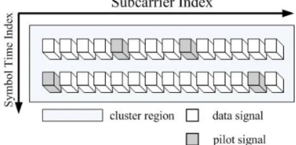
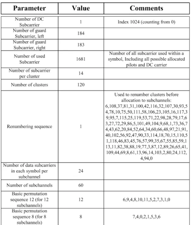
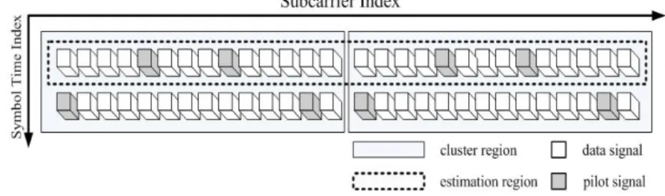
An OFDMA symbol is constructed with pilots, data and zero subcarriers. The symbol is first divided into basic clusters; pilots and data carriers are allocated within each cluster. Figure 2-9 shows the cluster structure with subcarriers from left to right in order of increasing subcarrier index. Table 2-1 summarizes the parameters of the OFMDA PUSC symbol structure, which takes the 2048 FFT size as an example.

Figure 2-9 Cluster structure

Allocation of subcarriers to subchannels is performed using the following procedure:

1) Dividing the subcarriers into the number of physical clusters containing 14 adjacent subcarriers in each symbol (starting from carrier 0).

formula:

( ) , first DL zones ((

13 _ ) mod _cluster) , otherwise RenumberingSequence PhysicalCluster RenumberingSequence PhysicalCluster DL PeermBase N LogicalCluster ⎧ ⎪ ⎨ ⎪+ ⋅ ⎩ = (2.15)

3) Dividing the clusters into six major groups. Group 0 includes clusters 0-23, group 1 clusters 24-39, group 2 clusters 40-63, group 3 clusters 64-79, group 4 clusters 80-103 and group 5 clusters 104-119. These groups can be allocated to segments. If a segment is being used, then at least one major group shall be allocated to it (by default group 0 is allocated to sector 0, group 2 to sector 1, and group 4 to sector 2).

4) Allocating subcarrier to subchannels in each major group as { [ mod ] _ }mod ( , ) subchannels k s k subchannels subchannels n p n N DL PermBase N subcarrier k s =N ⋅ + + (2.16) 5) where

z subcarrier k s( , )is the subcarrier index of subcarrier k in subchannel . s

z n_k =(k+ ⋅13 ) mods N_subcarriers

z N_subchannels is the number of subchannels (for PUSC use number of

subchannels in the currently partitioned group)

z p_s[ ]j is the series obtained by rotating basic permutation sequence cyclically to left times. s

z N_subcarriersis the number of data subcarriers allocated to a subchannel in each

OFDMA symbol.

2.2.3.2 DL FUSC

Similar to PUSC, the symbol structure is constructed using pilots, data and zero subcarriers. The symbol is first allocated with the appropriate pilots and with zero subcarriers, and then all the remaining subcarriers are used as data subcarriers. There are two variable pilot-sets and two constant pilot-sets. The variable set of pilots embedded within the symbol of each segment shall obey the following rule:

# 6 ( _ mod 2

PilotLocation VariableSet x= + ⋅ FUSC StmbolNumber ) (2.17)

where FUSC_SymbolNumber counts the FUSC symbols used in the transmission

Table 2-1 Parameters of the OFMDA PUSC symbol structure

2.2.4 DL Carrier Modulation

2.2.4.1 DL Pilot Modulation

In OFDMA, the polynomial for PRBS generator is 11 9 ₁

X

X + + , which is the

data tone. The pilot subcariers shall be modulated according to as 8 1 ( 3 2 { } { } 0 k k c c ) k ω − ℜ = ℑ = (2.18) 2.2.4.2 DL Data Modulation

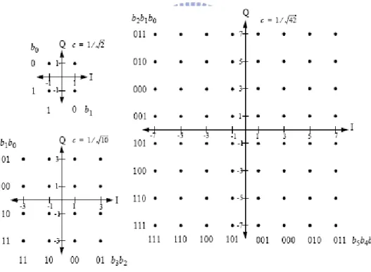
In the OFDMA system, Gray-mapped QPSK, 16-QAM and 64-QAM are supported, as shown in Figure 2-10. Each M bits (M=2, 4, 6) enter serially to form the constellation bits b(M-1)-b0 in MSB first order (i.e., the first bit should be mapped to the higher index bit in the constellation). Then, a constellation point is obtained with the plot in Figure 2-10.

2.3 Conventional Time-Invariant Channel Estimator

In this section, we will review some conventional channel estimators for OFDM system in time invariant channels. Here, we only consider pilot-aided systems, suitable for systems operated in mobile environments. Two channel estimation methods are well-known in OFDM systems, namely LS and MMSE. These methods can be applied to obtain the channel response either in the time or frequency domain. Except for the LS method in the frequency domain, these methods require to inverse a large matrix. Thus, the computational complexity is usually very high. In addition, the MMSE estimator needs to know the channel statistical characteristics, which is usually not available. When channel responses are estimated in the frequency domain, interpolation is required in general. The interpolation can be either one-dimensional or two-dimensional. We will discuss the problem of interpolation in Section 2.3.3.

2.3.1 LS Channel Estimator

The least-squares (LS) channel estimator is widely used in OFDM systems. It is the simplest estimator and is the foundation of the other advanced channel estimation methods. Using known pilot signals, we can estimate channel response on pilot locations. Let be the FFT size. The LS channel estimator minimizes the following squared errors [8]: N 2 ˆ LS − Y H X (2.19) where

[

₀, , ,_{1 1}

]

T N− =

Y Y Y _L Y is the frequency domain received signal vector,

[

0, 1, , 1

]

T N−

=

X X X _L X is the frequency domain transmitted signal vector, and. is an diagonal matrix minimizing Equation (2.19). Since the transmit data

ˆ

LS

H

Equation (2.19) as 2 , ˆ P − P LS P Y H X (2.20) where is the frequency domain received vector on pilot locations and is the frequency domain pilot signal vector,

is pilot location, and

0, 1, , M1 T P = ⎣⎡ m m m − Y Y Y _L Y ⎤⎦ ⎤⎦ 0, 1, , M1 T P = ⎣⎡ m m m − X X X _L X ,0 1 i i M

m ≤ ≤ − M is number of pilots. With the LS

algorithm [9], we then have

(

)

1 , ˆ H H P LS P P P P − = X X X Y H (2.21) Once we have the channel response at pilot tone locations, channel frequency responses in other tone locations can be estimated by interpolation.

The LS channel estimator also has a time-domain version. Rewriting Equation (2.20) in time domain, we can have

2 , ˆ

P− D P LS

Y X Gh (2.22) where X_{D P,} is diagonal matrix with the diagonal elements being

, is the DFT matrix, and is the channel response in the time domain. With the LS method, we then have

0 1 M-1 T m , m , , m ⎡⎣X X _L X ⎤⎦ G hˆLS

(

H H

)

-1 H H LS D,P D,P D,P P ˆ ₌ h G X X G G X Y (2.23)

and the LS error is defined as

ε

=Y_PH

(

I X G G X− _D,P

(

H _D,PHX G G X_D,P

)

-1 H _D,PH

)

Y_{P (2.24)}

As a result, the time domain channel impulse response can be estimated. However, this may require high computational complexity when the channel delay spread is large. This is because the matrix inside the parenthesis of Equation (2.23) is not diagonal anymore. We will propose a method to solve the problem in Chapter 3.

2.3.2

MMSE Channel Estimator

Linear minimum mean squared error (LMMSE) is a low-rank approximation result that uses the frequency-domain correlation of the channel [10]. It has been shown that LMMSE estimator is better than the LS method in OFDM systems. It minimizes the mean squared errors between the actual and estimated channels, obtained by a linear transformation. Channel frequency responses at pilot locations can be obtained as [9] 1 1 -1 , _{, , ,} , 2 , ˆ ˆ ˆ ( ( ) ) p LMMSE H H_{p p ZF} H_{p ZF}H_{p ZF} p ZF H H H_{p p} H H_{p p} σn p p p ZF − − = = + H R R H R R X X H (2.25)

where Hˆ _{p ZF,} is the zero-forcing algorithm ( _, p p ZF

p

= Y

H

X ) ,which is the LS solution

shown above (also called one tap frequency domain equalizer), 2

n

σ

is the variance of white Gaussian noise, X_p is the frequency domain pilot signal vector, and

{

_{, ,}

}

, , H H_{p ZF}H_{p ZF} =E Hp ZFHp ZF R (2.26)

{

H

}

H H_{p p} =E H Hp p R (2.27) As mentioned, once we have the responses at pilot tone locations, those at other tones can be estimated by interpolation.

The LMMSE channel estimator also has its time-domain version [11]. Observe the received signal after DFT shown below

Y X Gh W= _D + (2.28) where

[

₀, , ,_{1 1}

]

T

N−

=

Y Y Y _L Y is the frequency domain received signal vector and is frequency domain transmitted diagonal matrix, and

0 1 1

{ , , , }

D =diag −

variance 2

n

σ

). In pilot-aided systems, X_D can be separated into two parts, consists of pilot and data signals. Rewriting Equation (2.28), we have

Y=

(

ΦP_D +ΨS Gh W_D

)

+ 1 N 1 N (2.29) where is a diagonal matrix whose values are 0 except for pilot locations, is a diagonal matrix whose values are 0 except for data locations (

0 { , , } D =diag p p − P _L 0 { , , } D =diag s s − S _L k

p and s_k have the unity average power), 0

{ ,..., _N } diag φ φ ₋

Φ = ₁ is a diagonal matrix specifying the power for data tones, and

0

{ ,..., _N }

diag ψ ψ ₋

Ψ = ₁ for pilot tones. Assuming that V ΨS Gh= _D in Equation (2.29) is an interference, [9] gives the LMMSE estimate as

ˆ 1 (2.30) hY YY − = h R R Y where { H} H H H hY =E = h D R hY R G P Φ (2.31) _{ H_} H H H 2 2 (2.32) YY =E = D h D +μ +σn N R YY ΦP GR G P Φ Ψ I

In Equation (2.31) and Equation (2.32), { H}

h =E hh R , 1 2 0 / L l i N μ −σ = =

∑

and 2 n

σ

denotes the variance of the AWGN. Here, L is the maximum channel delay spread. As we can see, the LMMSE estimator requires higher computational complexity than the LS estimator. Still, it needs to know the channel statistical characteristics which are usually not available in real-world applications.

2.3.3 Frequency Domain Interpolation Methods

As discussed, channel responses in the frequency domain can be obtained in pilot tone positions. To obtain response in data tone positions, we need to use the interpolation technique. Note that the interpolation is highly system dependent; different pilot allocation methods result in different interpolation strategies. In this section, we will introduce dome interpolation techniques and explain how to deal with different systems.

The interpolation problem involves two-dimensional operations, i.e., operations in the frequency temporal domains. The dimension in frequency domain is defined by the subcarrier index, and the temporal domain is the symbol time index. Note that the channel delay spread determines how fast the channel response varies in the frequency domain. It is difficult to obtain a good interpolator if the channel response variation is large. The classical approach for channel interpolation is to construct a polynomial interpolator fitting responses in known samples. The polynomial interpolator can be formulated in various ways, such as the power series, Lagrange interpolation and Newton interpolation. These various forms are mathematically equivalent and can be transformed from one to another. Assume that samples are available, denoted as

1

N+

0 1

{ ( ), ( ), , ( )}x t x t _L x t_N , where x t( )_n is the amplitude of the

signal x t( ) at time . The polynomial with order , passing through the known samples, can be written in a power series form as

n t N N+1 1 2 0 1 2 ( ) ˆ( ) _N N N t x t =P =a +a t +a t + +_L a t (2.33)

Figure 2-11 A polynomial interpolator

Note that the polynomial is unique (see in Figure 2-11). Using Equation (2.33) and a set of known samples, we can solve the polynomial coefficients by

linear equations which can be formulated as a matrix form:

1 N+ a_k N+1 1 2 0 0 0 0 0 2 1 1 1 0 1 2

( )

1

( )

1

( )

1

N N N N N N N N

a

t

t

t

x

a

t

t

t

x

a

t

t

t

x

−

⎡

⎤

t

t

t

⎡ ⎤

⎡

⎢

⎥

⎤

⎢ ⎥

⎢

⎢

⎥

⎥

⎢ ⎥

₌

⎢

⎢

⎥

⎥

⎢ ⎥

⎢

⎢

⎥

⎥

⎢ ⎥

⎢

⎢

⎥

⎥

⎣ ⎦

⎣

⎦

⎣

L

L

M

M M

M

O

M

M

L

⎦

(2.34)

The matrix in Equation (2.34) is called a Vandermonde matrix. The dimension of the matrix becomes large when N is large; its inverse is then difficult to compute. For this reason, the polynomial order used is usually small (e.g., linear or quadratic interpolation).

For signals in pilot tones, we can rewrite Equation (2.34) as:

x Ta= (2.35) 2 1 0 0 0 0 0 2 1 1 1 1 1 0 2 1 1 1 1 1 1 1 1

( )

1

( )

1

(

)

1

N N N N M M M M M M N N

a

x t

t

t

t

a

x t

t

t

t

a

x t

t

t

t

− − − − − − − − × × ×

⎡

⎤ ⎡

⎤

⎡

⎤

⎢

⎥ ⎢

⎥

⎢

⎥

⎢

⎥ ⎢

⎥

⎢

_{⎥ =}

⎢

⎥ ⎢

⎥

⎢

⎥

⎢

⎥ ⎢

⎥

⎢

⎥

⎢

⎥

⎣

⎦

⎣

⎦

⎣

⎦

L

L

M

M

M

M

M

O

M

L

(2.36)

where [ ( ), ( ), , (_{0 1 1})]T is the pilot signals and

M

x t x t x t ₋

=

pilot signals, is the polynomial coefficient, and is the order of polynomial interpolator. Note that in Equation (2.36) is no longer a Vandermonde matrix. Also, it becomes overdetermined since

0 1 1

[ , , ,

]

T N

a a

a

₋

=

a

_L

N T M is usually larger thanN . So the polynomial coefficient can be solved by the LS algorithm as: a

1

( H )− H

=

a T T T x (2.37) The simplest polynomial interpolator is the first-order polynomial interpolator. However, the performance is usually not satisfied. The quadratic interpolator is a second-order polynomial interpolator. It can have better performance in general. Since the number of unknowns is larger, more pilots are also required. Consider the cluster structure in the IEEE 802.16e system in Figure 2-9. As we can see, only 2 pilot signals are available in a single OFDM symbol. In order to have a quadratic estimate, at least we have to use two clusters at a time such that 4 pilot signals can be used. Using Equation (2.37), we can then obtain the polynomial coefficients with the LS algorithm. Finally, all frequency response across two clusters in a single OFDM symbol can be evaluated with the fitted quadratic function. The estimation scheme is shown in Figure 2-12.

Figure 2-12 Channel estimation with 2-cluster quadratic interpolator

The method mentioned above is a one-dimensional interpolation approach, which only uses one OFDM symbol. Although a higher order may have better results,

reduce the effectiveness of the interpolation. Another way to enhance the interpolation performance is to use a two-dimension interpolator.

In [12], a simple method has been proposed to perform a two-dimension interpolation in the IEEE802.16e system. The two-dimension interpolator is separated into two one-dimension polynomial interpolators; one is linear and the other is quadratic. Since the frequency response varies slowly with time, the interpolation between OFDM symbols is linear. This method is called a Linear and Quadratic (LAQ) method.

The basic idea of the method is to use pilot signals from other clusters to aid the interpolation in a particular cluster. From Figure 2-9, we can see that the pilot signals in consecutive clusters (along with the symbol time index) are only decimated by a factor of two. Thus, we use a linear interpolation, averaging two consecutive pilot signals, to obtain the one in between. By doing so, 2 extra (pseudo) pilot signals are obtained in a cluster. Figure 2-13 shows the operation described above. Now, there are 4 pilot signals in a cluster. The matrix-vector form in Equation (2.36) can be reformulated as 2 0 0 0 0 2 1 1 1 1 2 2 2 2 2 2 3 1 3 3 3 4 1 4 3

( )

1

( )

1

( )

1

( )

1

x t

t

t

a

x t

t

t

a

x t

t

t

a

x t

t

t

× × ×

⎡

⎤

⎡

⎤

⎡ ⎤

⎢

⎥

⎢

⎥

⎢ ⎥

⎢

⎥

⎢

_{⎥ =}

⎢ ⎥

⎢

⎥

⎢

⎥

⎢ ⎥

⎢

⎥

⎢

⎥

_{⎣ ⎦}

⎢

⎥

⎣

⎦ ⎣

⎦

(2.38)

where is channel response of the vector of 4 pilot signals, are location index of the 4 pilot signals (1,5,9,13, respectively), and is the polynomial coefficient vector. Using Equation (2.37), we can then obtain the polynomial coefficients by the LS method.

x { , , , }t t t t_{0 1 2 3}

Chapter 3

Proposed Channel Estimators

In Chapter 2, we have reviewed some channel estimation methods for the pilot-aided OFDM systems. Specifically, we have described the LAQ frequency-domain channel estimator developed for the IEEE 802.16e system. Although the LAQ interpolation method can have good performance, the results in the boundary areas of a cluster may not be satisfactory. This is because channel responses interpolated in those areas only use one-sided data. In this chapter, we will first propose a modified LAQ interpolation to solve the problem. The details are discussed in Section 3.1.

Due to limited pilot signals, channel estimation in frequency domain interpolation will be degraded when channel delay spread is large. In this case, the interpolation method cannot recover the frequency response completely, even with a high order of polynomial. For this reason, we focus the channel estimation in time domain approach. However, the conventional MMSE and LS channel estimator in time domain require high computational complexity. In addition, the MMSE channel estimator needs to know the channel statistical characteristics, which are usually not available. In this Chapter, we will develop a high-performance yet low-complexity LS channel estimator. This method works well with large channel delay spread and high

mobile speed. In typical wireless channels, the delay spread may be large, but the number of non-zero taps is small. The key idea of the proposed method is locate and estimate the responses at non-zero positions. Detailed description can be found in Section 3.2 and Section 3.3. Combining both temporal and frequency domain operations, we finally propose an efficient channel estimator. A recursive procedure is also introduced to further reduce the complexity and improve performance. The details are discussed in Section 3.4.

In high-speed mobile communications, the coherent time of the channel can be less than an OFDM symbol duration. In this case, the channel in the OFDM symbol is not time-invariant anymore, and ICI effect is introduced. Many ICI suppression methods have been proposed recently [13]-[15]. All the methods rely on good channel estimates. For the last section of this chapter, we extend the method developed in Section 3.4 and propose a low-complexity time-variant channel estimator. The details are discussed in Section 3.5.

3.1 Sliding-Windowed LAQ Channel Estimator

As mentioned in Section 2.3.3, the LAQ interpolation method (as shown in Figure 2-13) has been developed for the IEEE 802.16e system. In the determination of the order of the polynomial, two aspects must be considered. First, the number of pilot signals must be larger than the order of the polynomial to make sure the matrix is over-determined (see Equation 2.37). Second, the order of the polynomial must be high enough such that it can properly describe the frequency response variation, which depends on the maximum channel delay spread. The LAQ interpolation method chooses the quadratic function to conduct channel estimation, compromising these two factors.

T

Although the LAQ interpolation method can have good performance, the results in the cluster boundaries may not be satisfactory. This is because channel responses interpolated in the areas only use one-sided data. As a result, the boundary areas will be discontinuous as shown in Figure 3-1. In the figure, the estimation result with the LAQ method is denoted by the solid curve, the discontinuousness in the boundary areas is indicated by the dashed box.

Thus, the LS fitting in Equation (2.37) may not be optimal for tones in both cluster ends. For this reason, we propose an extended method, called the sliding window method, to remedy this problem. The method is depicted in Figure 3-2, and the corresponding operations are summarized in the following steps:

1) Select a window size (the dashed box in Figure 3-2).

2) Use the channel responses of pilot and pseudo pilot signals in the window, and construct the matrix in Equation (2.36). Then, use the LS algorithm to obtain the polynomial coefficient vector . a

3) Calculate the frequency response in the output region (the colored part in Figure 3-2) by the LAQ interpolation method, and output the estimates in the region.

4) Slide the window along the subcarrier index by tones and then go to 2) until the subcarrier index reach its maximum.

This extended interpolation method can solve the problem mentioned above and the performance can be further enhanced, though its computational complexity is somewhat higher than conventional LAQ interpolation method. The window length, the output region, and the step of sliding are parameters needed to be determined. The Simulation results are shown in Chapter 4.

3.2 Low-Complexity Time Domain Channel

Estimator

We have described the conventional time domain LS channel estimator in Section 2.3.1. Figure 3-3 illustrates the equation for OFDM receive signal in frequency domain. With the pilot-aided system, we take the signals on pilot locations (the grey area in Figure 3-3) to fit the LS channel estimate. The estimated time domain channel impulse response is shown in Equation (2.23). Since the solution involves a matrix inversion, we require

( )

3

L

Ο arithmetic operations where L is

the maximum channel delay spread. In OFDM systems, is usually the CP size which is large in general. As a result, the required computational complexity is large. We now take the advantage of a property in typical wireless channels to develop low-complexity algorithms. In outdoor wireless environments, the number of major multipath reflections is usually limited. In other words, the number of non-zero channel tap is small, though the delay spread may be large. Let the number of these particular taps be

L

L%, which is always much less than L. The number of unknowns

to be solved is L% instead of L. (the dotted area in Figure 3-3). Then the channel impulse response on particular position can be estimated by Equation (2.23) and only requires

( )

3 arithmetic operations [16].

L Ο %

The only problem is we need to locate the channel tap positions which have significant values. Using this approach, we can estimate channel more precisely, and reduce the computational complexity significantly. How to locate the channel tap positions will be introduced in next section.

Figure 3-3 Equation for OFDM receive signal in frequency domain

3.3 Channel Tap Search Algorithm

In this section, we propose two methods to locate significant (nonzero) channel taps. The idea is to construct a preliminary time-domain channel impulse response first, and then locate the significant taps by some searching algorithm. Finally, we can estimate the response at those taps by the LS method. The details are described below.

3.3.1 Preliminary Channel Estimation with Preamble

The preamble is the first symbol of the downlink OFDM transmission. A simple way to construct the channel impulse response is using the preamble, which is the known sequence. Consider the preamble passing through a multipath channel, which is shown in Figure 3-4(a). Because of the multipath effect, the received signal will be a superposition of signals from different delay paths and AWGN. We can then conduct the correlation operation between the received signal and the known preamble (as shown in Figure 3-4(b)). When the preamble matches the original signal, the peaks can then be located. Since the channel responses are complex, we will use their absolute values in the peak detection.

Figure 3-4 Preliminary channel estimation (with preamble)

The correlation operation can be made equivalent to the convolution operation. So, the procedure can be transformed to frequency domain.

h⊗ ⊗ =f f IFFT H F F{ ⋅ ⋅ } (3.1) where and are the channel response respectively in the time and frequency domains, and

h H

f and F are the preamble sequence respectively to in the time and

frequency domains. We can then multiply the received signal and the preamble in the frequency and transfer the result back to the time domain to replace the time-domain correlation operation. However, not all communication systems have the preamble structure. So, we will introduce another method to search channel taps.

3.3.2

Preliminary Channel Estimation with Pilots

The time-domain channel impulse response can be constructed if its frequency-domain response can be estimated. In pilot-tone systems, the channel frequency response can be estimated and interpolated as discussed in Section 3.1. Since we only need to know the rough channel impulse response shape, we can take the IFFT of the interpolated channel response (see in 2.3.3) to obtain the time-domain response. Based on the result, we can then locate peaks of channel impulse response.

3.3.3

Channel Tap Search Method

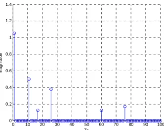
Here, we propose two simple methods to locate the positions of significant channel taps. Figure 3-5 shows the result of the preliminary channel estimation using the preamble of the IEEE802.16e. We can clearly see the peaks of the channel response. Furthermore, the channel tap is complex value so we only see the magnitude part. -5 0 5 10 15 20 25 30 35 40 45 0 0.1 0.2 0.3 0.4 0.5 0.6

Figure 3-5 Result of the preliminary channel estimation

The first method is simply to compare the value of a tap with a threshold. If it is larger than the threshold, the tap is deemed as a peak (significant tap). Otherwise, it will be considered as a zero tap (Figure 3-6). As we can see, there is a low-passed signal embedded in the channel response. So some fake taps will occur near the significant taps (the gray line in Figure 3-6). For this reason, the threshold will be difficult to determine and the smaller taps may not be detected.

The second method takes a first-order differentiation to the channel response. As a result, the low-passed signal will be removed. We can then compare the result with a threshold. The tap with a value higher than the threshold is deemed as a significant tap. Note that, a significant tap will result two peaks; one is positive and the other is negative (Figure 3-7). We need only consider the positive one. The definition of the differentiation operation is given by

d k[ ]=h k%[ + −1] h k%[ ] (3.2)

Figure 3-7 Channel tap searching method by first-order differentiation

However, consecutive channel taps may not be detected. For this reason, we further propose a more robust method for the detection. The idea is to locate the taps in an iteratively manner, rather than in one short. Figure 3-8 shows the iterative procedure. First, locate channel taps with Method 1 or 2 with a higher threshold value. In this case, smaller or consecutive taps may not be detected. Then, remove the located channel taps from the channel response (as shown in Figure 3-8(a)), and relocate taps (the threshold may be changed). Repeat this process until no more taps are detected. With proper thresholds, this iterative method we can almost locate all channel taps correctly.

Figure 3-8 Iterative channel tap searching method

3.4 Joint Time and Freq Domain Channel Estimator

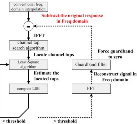
In Section 3.2, we propose a modified time-domain LS channel estimator for channels with known tap positions. In Section 3.3, we proposed two channel tap search algorithms; one uses the preamble and the other uses pilots. In IEEE802.16e system, the channel response estimated with the preamble may not be able to be applied in the following data bursts since the receiver is mobile. For this reason, we only consider the preliminary channel estimation using pilot signals. Since the Method 2 for the tap search performs better, we use that in following development. Combining the preliminary channel estimation, the channel tap search algorithm, and the modified time-domain LS channel estimator, we are able to obtain a low-complexity yet high-performance channel estimator. We called this a joint time and frequency domain channel estimator. The estimation flowchart is shown in Figure 3-9. The procedure is summarized as follows:

Figure 3-9 Proposed channel estimation flowchart

1) Use the conventional frequency domain interpolation method to obtain the preliminary channel frequency response.

2) Take the IFFT of the response to the time domain, and then locate significant channel taps (the threshold is iteration dependent).

3) Use the LS algorithm to estimate channel impulse response in those taps.

4) Compute the least-squared error (LSE) with a threshold. If the LSE is greater than the threshold, reconstruct the frequency response of those located taps by FFT, and force the response in the guardband region to zero. Then, subtract it from the original channel frequency response, and go to step (2). If LSE is smaller than the threshold, stop the iteration.

Note that the LSE is a good indicator telling us when to stop the searching. In other words, it can avoid the redundant channel taps to be detected and reduce the computational complexity for the LS algorithm. In mobile environments, the channel tap positions may change with time slowly or suddenly. The LSE can also help us to

check channel tap positions have changed or not.

The iteratively operation not only locates the channel taps more precisely, but also requires reduces computational complexity of the LS algorithm. However, a FFT/IFFT operation is required for each iteration and this will increase the computational complexity significantly. This can be remedied with the following approach. The main idea is to transfer the response-subtraction operation in the frequency domain to the time domain. Note that the operation conducted in the frequency domain is windowing and subtraction, which can be transferred into convolution and subtraction in the time domain. The function to be convolved is the sinc filter. In practice, the sinc filter may be difficult to implement. So, we may replace it by some lowpass filter. Since the number of detected taps is expected to be small, the required computational complexity of the convolution operation will not be significant. The modified flowchart is shown in Figure 3-10.

3.5 Time-Variant Channel Estimation

The maximum Doppler spread of a mobile station is shown to be

C D v f f c ⋅ = (3.3) where is the mobile speed, v f_C is the carrier frequency, and is the speed of

light. The coherent time is known to be the inverse of Doppler spread (

c C t _C 1 D t f ≅ ). If the mobile speed is high, the coherent time becomes small. When the coherent time is less than an OFDM symbol duration, the channel in the OFDM symbol is no longer time-invariant. As a result, intercarrier-interference (ICI) effect will be induced, degrading the system performance. There is a considerably amount of research in ICI mitigation. It has been known that the performance of ICI mitigation heavily depends on the accuracy of channel estimation. In this section, we focus on the estimation of time-variant channel. We will extend method proposed in previous sections to obtain a low-complexity and high-performance algorithm.

In [15], a linear time-variant channel model is used to develop a simple channel estimation method. The received signal with ICI effect is modeled as

(3.4) 1 ,0 , (( )) 1 ,0 1 N N i i i i d i d i d Y H X H X W i N − − = = +

∑

+ ≤ ≤ −

where is the received signal in the frequency domain, is the transmitted signal in the frequency domain, denotes the FFT of the AWGN, and is the FFT size. The middle term in the right hand side of (3.4) represents the ICI term. It has been shown in [15] that can be seen as the frequency response of an equivalent channel, averaging the channel taps over the time duration of

. Let be the averaged time-domain channel tap. Thus,

Y X

W

N ,0 ˆ i H 0≤ < ×t N T_S h_kave _kth 2 1 ,0 0 1 ˆave L ˆ j Lik_{,0 1} i k i h H e k L L π − = =

∑

≤ ≤ − (3.5)

where L is the length of channel. Note that Hˆi,0 can be estimated with Y Xi / i.

Using the model, we can treat the channel as a time-invariant channel with time domain taps ’s (Its frequency response is ). Thus, the channel estimation proposed in previous sections can be applied directly. In typical channels, the variation of channel taps is small. In an OFDM symbol, it is reasonable to assume that the channel tap variation is linear (as shown in Figure 3-11).

ave k

h Hˆ_i,0

Figure 3-11 Linear approximation of time-variant channel

With the model, it is simple to see that ( ave s2

k k

E h −h ) is minimized for

( 2 1)

N

s= − , proved in [15]. Thus, we can let h_kave be equal to (2 1)

N k h − (as shown in Figure 3-12). ˆ(2 1) N ave k h − = ˆh_k (3.6) ,

ˆ

ave k i

h

, 1

ˆ

ave k i

h

₊ ( 1) 2 ,

ˆ

N k i

h

− ( 1) 2 , 1

ˆ

N k i

h

₊−

0

iT

( 1)i+ T