國
立
交
通
大
學
資訊科學與工程研究所
碩
士
論
文
非等向性散射之光影模型及其即時顯像
A Real-Time Analytic Lighting Model for Anisotropic
Scattering
研 究 生:洪凱生
指導教授:莊榮宏 教授
林正中 教授
Anisotropic Scattering
by Roger Hong
A dissertation submitted to the faculty of National Chiao Tung University in partial sat-isfaction of the requirements for the degree of Master of Science in the Department of Computer Science.
Committee in charge: Professor Jung-Hong Chuang
Professor Yung-Yu Chuang Professor Chun-Fa Chang
Copyright 2006 by Roger Hong
A Real-Time Analytic Lighting Model for Anisotropic Scattering
Student: Roger Hong Advisor: Jung-Hong Chuang
Department of Computer Science National Chiao Tung University
Abstract
Rendering the effects of light scattering for interactive applications is often made difficult by the demands of dynamic viewing, lighting, scene geometry, and environment parameters. Recent advances in rendering of participating media using analytic techniques have enhanced performance significantly to meet this challenge, albeit under assumptions and simplifications made to scenes. In this thesis, we present an analytic lighting model for dynamic, accurate, and single anisotropic scattering that may be used for scenes such as fog, mist, or haze. Our model applies an explicit analytic integration to an angle-formulated single scattering integral for a point light source in a homogenous participating medium. Users may create a dynamic scattering environment, such that scattering conditions may be controlled using simple parameters for density and forward scattering level. Using this model, we demonstrate the effect of forward scattering on glows around light sources and surface radiance. The method can be implemented on programmable graphics hardware in real-time.
To my family,
for abounding encouragement and levity.
Contents
List of Figures iv List of Tables v 1 Introduction 1 1.1 Motivation . . . 2 1.2 Contribution . . . 2 1.3 Limitations . . . 4 1.4 Organization . . . 42 Light Scattering for Computer Graphics 5 2.1 Phase Functions and Anisotropic Scattering . . . 6
2.1.1 Rayleigh Scattering . . . 7
2.1.2 Mie Scattering: Henyey-Greenstein Phase Function . . . 7
2.2 Light Scattering Terminology . . . 8
2.2.1 Absorption, Emission, Scattering, and Extinction . . . 8
2.2.2 Transmittance and Optical Thickness . . . 10
2.3 Integral Transport Equation . . . 11
2.3.1 Simplifying Assumptions . . . 12
3 Related Work: Interactive Rendering of Light Scattering Effects 16 3.1 Numerical Methods . . . 17
3.1.1 Shafts of Light and Volumetric Shadows . . . 17
3.1.2 Atmospheric Effects . . . 18
3.1.3 Multiple Scattering . . . 19
3.2 Analytic Methods . . . 21
3.2.1 Effects for Point Light Sources . . . 21
3.2.2 Sky and Terrain Rendering . . . 23
4 Analytic Lighting Model for Accurate and Dynamic Anisotropic Scatter-ing 25 4.1 Introduction . . . 26
4.2 Analytic Lighting Model . . . 27
4.2.2 Surface Radiance Model using Angle Formulation . . . 30
4.2.3 Summary of Analytic Lighting Model . . . 35
4.3 Dynamic Anisotropic Scattering . . . 37
4.4 Hardware Implementation . . . 40
5 Experimental Results 44 5.1 Visual Effects of Anisotropic Scattering . . . 44
5.2 Rendering Test Scenes . . . 47
6 Conclusion 51 6.1 Summary . . . 51
6.2 Future Work . . . 52
6.2.1 Analytic Model for Scattering from Anisotropic Light Sources . . . . 52
6.2.2 Volumetric Shadows . . . 53
List of Figures
2.1 Henyey-Greenstein phase function for g = 0.5 . . . . 8
2.2 Diagram of single scattering integral for point light source . . . 15
2.3 Diagram for single scattering integral of atmospheric model . . . 15
4.1 Diagram illustrating light paths . . . 27
4.2 Diagram for angular reformulation of the airlight integral . . . 28
4.3 3D plot of precomputed function H(u, v) . . . . 30
4.4 Diagram for surface radiance integral . . . 31
4.5 3D plots of precomputed functions J1(T sp, θs) and J20(Tsp, θ0s) . . . 34
4.6 Illustrative summary of analytic lighting model of Section 4.2 . . . 36
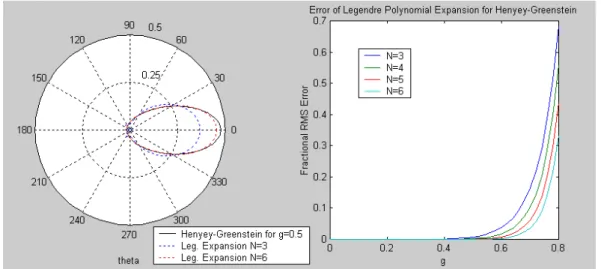
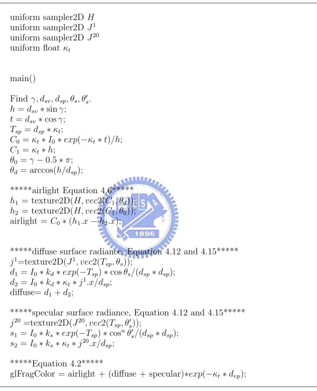
4.7 (left)Normalized Henyey-Greenstein phase function and its Legendre polyno-mial expansion. (right)Rms error plot of Legendre polynopolyno-mial approximation 40 4.8 Fragment shader pseudocode for version without dynamic anisotropic scattering 42 4.9 Fragment shader pseudocode for version with dynamic anisotropic scattering 43 5.1 Glows around light sources in and out of direct view for varying forward scattering conditions . . . 45
5.2 Specular radiance and diffuse radiance for varying forward scattering conditions 46 5.3 Test Scene: varying densities . . . 48
5.4 Test Scene: varying forward scattering . . . 49
5.5 Images of pavilion scene. . . 50
5.6 Images of atrium scene. . . 50
6.1 Diagram of scattering with anisotropic light source . . . 53
6.2 Diagram for volumetric shadow algorithm . . . 55
6.3 Image of torus’ volumetric shadow . . . 56
6.4 Image of table’s volumetric shadow . . . 57
6.5 Image illustrating problem when there are intersecting shadow polygons . . 57
6.6 Image illustrating clamping problems . . . 58
List of Tables
4.1 Notation and formulae for angle-formulated airlight integral . . . 28
5.1 Table of rendering speeds as a function of number of light sources . . . 47
Acknowledgments
I would like to thank my advisors, Professor Jung-Hong Chuang and Professor Cheng-Chung Lin, for their guidance and patience. Instilling a focus to my research proved invaluable. An appreciative thanks goes to Tan-Chi Ho for his continual help from the very beginnings to the latter stages . I am fortunate he makes himself readily available. I would also like to thank Yu-Hsian Sun for sparking what became the topic of my thesis. Thanks to Ya-Ching Chiu for painstaking translation work along the way. A big thanks to the entire group: Yi-Chun Lin, Chao-Wei Juan, Yong-Cheng Chen, Chen-Li Hao, Yu-Shuo Lio, Chia-Lin Ko, Ji-Wen Chon, and Yung-Cheng Chen. You guys answer every last question of mine. Thanks to Jyh-Shyang Chang for modeling help under short notice. Thanks to Warren Lin for proofreading and tums. Lastly, I would like to thank my parents for grounding me then lifting me when the time was right.
Chapter 1
Introduction
Rendering effects of light scattering in atmospheric environments has long been a field of interest within the computer graphics community. Light scattering, caused by particles such as water or dust in the air, creates visual effects including visibility loss, glows around light sources, blurred surface radiance, shafts of light, and volumetric shadows. All these visual cues add to the realism of scenes with participating media. The computation of light transport in volumetric environments, however, presents a challenge for developing practical, interactive rendering methods for participating media in computer graphics.
Recent advances in consumer graphics hardware in both speed and flexibility, es-pecially the ability to run code at the vertex and fragment level, have spurred the growth of methods for real-time rendering of scenes with participating media to meet this chal-lenge. Much of the research for interactive rendering of participating media focuses on how to best exploit important hardware capabilities to solve complex scattering equa-tions. Rectangular meshes storing illumination terms at lattice points can be used to render effects such as volumetric shadows and shafts of light [Dobashi et al., 2000a], al-though scene-dependent banding artifacts caused by undersampling may occur. Glows around point light sources can be rendered in real-time for scenes with fog and volu-metric shadows [Biri et al., 2006], but banding artifacts occur when the viewer to very close to a source. Based on a particle system, a complete real-time rendering system for clouds [Harris and Lastra, 2001] allows the viewer to fly in and out for applications such as in
flight simulators. The precomputation of illumination required, however, is scene dependent and can widely vary. The advent of programmable graphics hardware has spawned numerous works exploiting its flexibility. These include methods for real-time atmospheric scattering effects [Hoffman and Preetham, 2003, O’Neil, 2005], but uniform density must be assumed. Also, interactive multiple scattering effects for inhomogeneous media [Hegeman et al., 2005] are demonstrated, although large amounts of scene-dependent precomputation is required. Complex scattering effects on surface radiance [Sun et al., 2005] have been made possible in real-time, but only scenes under the assumption of isotropic scattering is demonstrated. This work deals specifically with anisotropic scattering within the context of ren-dering participating media for computer graphics applications. Thus, it is concerned with the variation of atmospheric conditions that result from the interaction of light and dif-ferent particles in the atmosphere. Difdif-ferent anisotropic scattering conditions are seen in everyday life, including that of fog, mist, haze, or rain. Accurately modeling this type of scattering behavior adds to the visual realism desired in many interactive computer graphics applications.
1.1
Motivation
Rapid advances in consumer graphics hardware has allowed researchers to branch into interactively rendering volumetric environments, no longer restricted to only rendering of surfaces. As such, the overall goal of this work is to develop a practical rendering method for real-time graphics applications that considers increasingly complex scattering effects and dynamic behavior.
1.2
Contribution
We present, over the course of this thesis, a real-time analytic lighting model that is able to handle anisotropic scattering accurately as well as complex visual effects including glows around light sources and effects on surface radiance in scenes with fog, mist, or haze. Previous works either have ignored these complex visual effects or were unable to handle
anisotropic scattering accurately. Furthermore, we extend the lighting model to introduce a
dynamic scattering environment, such that the scattering conditions of an atmosphere can
be manipulated by the user in real-time. The visual appearance of scenes with scattering environments are no longer limited by pre-determined implementation choices. The user may dynamically control the scattering environment using simple parameters of density and forward scattering, generating a limitless variation of scattering conditions as well as receiving instant visual feedback. By using our lighting model, we are able to demonstrate the visual effects of forward scattering on glows and surface radiance. The entire implemen-tation for our model using programmable graphics hardware is detailed and demonstrated in this work.
It focuses on the visual effects present in scenes with fog, mist, and haze, such that the viewer and light sources are both immersed within the medium. It is especially effective for near-field scenes in which the viewer and light sources are in close proximity. Specifically, our model considers effects of scattered radiance emanating directly from light sources, commonly termed airlight. The model captures effects for variable levels of forward scattering on glows around light sources, diffusing of specular highlights, and shadowed regions. The scattering behavior of the model may be dynamically controlled by just two simple parameters, the forward scattering parameter g and the extinction coefficient κt of the scattering medium. A precomputation step that is entirely independent of the physical parameters of the scene enables the dynamic behavior. Furthermore, the model can be easily integrated into an existing real-time rendering framework. More precisely, we develop an analytic model for single scattered radiance reaching the viewer for a point light source in a homogenous medium. The model may use any phase function of a single parameter
θ without significant effect on run-time performance or loss in accuracy, thus making it
appropriate as a general model for anisotropic scattering.
This work can largely be viewed as an application of the methodology used in [Sun et al., 2005] towards an alternative angle-formulated version of the single scatter-ing light equations, whereby we obtain new results that enables efficient and accurate anisotropic scattering. In addition to dynamic lighting, geometry, and density of the medium of the previously mentioned work, we introduce dynamic forward scattering, which is
pre-sented as an extension to an initial analytic solution.
1.3
Limitations
To achieve interactive rates, the physics-based lighting model is restricted to single
scatter-ing, the assumption that light scatters only once in the medium. In environments with low
albedo, single scattering is a reasonable approximation [Cerezo et al., 2005]. The demands typical in interactive applications such as dynamic viewing, lighting, scene geometry, and environment parameters require the model to assume isotropic point light sources, homo-geneous media, and single scattering.
Although the use of scattering equations in this work is physically-based, visual appeal is the primary goal of the work, as opposed to strict, physical-simulation-like ac-curacy. This is not to say accuracy is not important, as it significantly affects the visual realism of scenes–the ability of the eye to perceive subtle visual cues in scattering environ-ments is rather impressive. Such is the case with different levels of forward scattering(i.e. the difference between fog, mist, or haze)–though the average observer may have difficulty describing the visual difference among varying scattering conditions, he will invariably per-ceive a difference.
1.4
Organization
This thesis is organized as follows. Chapter 2 describes background in light scattering necessary for computer graphics. Chapter 3 describes related works regarding the interac-tive rendering of light scattering effects. Chapter 4 presents the proposed lighting model for accurate and dynamic anisotropic scattering as well as the hardware implementation. Chap-ter 5 describes the results of our method, including a qualitative description of anisotropic scattering effects. Finally, Chapter 6 concludes this work, describing limitations, possible areas of future work, and a summary.
Chapter 2
Light Scattering for Computer
Graphics
When light travels through an environment, it interacts with particles of various sizes within the volume of space, a phenomenon known as light scattering. When the number of interactions is low, such as when there exists low density, small particles, or a short distance to be considered, light scattering can be ignored altogether. But in scenes with participating media, light scattering must be considered if visual realism is a desired result.
In this chapter, some background necessary for rendering light scattering effects is discussed. Firstly, a discussion of scattering distributions described by phase functions is presented. Phase functions will be more formally defined and elaborated on for use in describing various real-world scattering conditions. Secondly, the basic volumetric scatter-ing processes of absorption, emission, scatterscatter-ing, and extinction will be introduced. These processes form the building blocks necessary for considering how to render complex scatter-ing environments. In the same section, other scatterscatter-ing terminology will be defined to be used in the rest of this work. Lastly, a general model for rendering light scattering effects in computer graphics, the integral transport equation, will conclude the chapter.
Before entering the discussion of this chapter, basic knowledge of the radiometric quantity, radiance, is assumed. It is defined as the radiant power per unit area, per unit
solid angle, and largely determines the quantity used for computer graphics display.
2.1
Phase Functions and Anisotropic Scattering
The appearance of participating media is affected by both the size and density of particles, among other factors. The size of particles primarily determines light scattering distributions. That is, when there is a light-particle interaction, light scatters in different directions to varying degrees. In computer graphics, light scattering distributions are modeled using
phase functions. The simplest model assumes isotropic scattering, in which light scatters
equally in all directions. This, however, is insufficient for real-world conditions. Therefore, modeling anisotropic scattering, in which light scatters non-uniformly, is a challenge our work undertakes.
More formally, the phase function p(ωi, ωo) describes the angular distribution of
scattered radiation at a point. A dimensionless quantity, it determines how much light with incoming direction ωi is scattered into outgoing direction ωo. The normalization constraint
allows the phase function to define the probability distribution for scattering in a particular direction, written as:
1 4π
Z Ω4π
p(ωi, ωo)dωo = 1 (2.1)
Another property of phase functions is that they are reciprocal (i.e. p(ωi, ωo) = p(ωo, ωi)).
Because most phase functions for interactive computer graphics are symmetric about the incident direction, scattering distributions can be parameterized by the single angle θ between ωi and ωo, such that a common notation for phase functions is p(θ).
Uni-form scattering defined by a constant phase function, p(θ) = 1
4π, is termed isotropic
scatter-ing. Scattering defined by a non-constant phase function is termed anisotropic scatterscatter-ing.
Descriptions of common phase functions used to model different scattering conditions in computer graphics compose the rest of this section. Certainly, more complex phase func-tions not mentioned in this chapter exist, mostly seen in non-interactive works. One may look to [Pharr and Humphreys, 2004, Premoze et al., 2003] for further reference.
2.1.1 Rayleigh Scattering
The Rayleigh scattering model is appropriate for describing the distribution found in the earth’s atmosphere for very small particles with size less than the wavelength of light. In this type of scattering distribution, particles scatter in the forward and backward direction equally. Rayleigh scattering exhibits an important property: dependence on wavelength λ. The amount of scattering is proportional to λ14. Therefore, light with shorter wavelengths
scatters more frequently, causing it to bounce everywhere and yield the color of the blue sky. This is also why one observes colors of longer wavelengths such as orange and red during the sunset because all of the longer wavelengths of light have scattered away before reaching the observer. A simple phase function widely used for Rayleigh scattering is
p(θ) = 3
16π(1 + cos
2θ) (2.2)
One set of wavelength scattering coefficients(constants) used is 6.95×10⁻⁶m−1for red light,
1.18×10⁻⁵m−1 for green light, and 2.44×10⁻⁵m−1for blue light [Preetham, 2003]. Further
discussion of these coefficients can be found in the referenced work.
2.1.2 Mie Scattering: Henyey-Greenstein Phase Function
Mie scattering describes the scattering distribution for large particles in atmospheres with fog, mist, or haze. It is largely wavelength independent and exhibits strong forward scat-tering. The Henyey-Greenstein phase function is commonly used to describe Mie scattering distributions due to its simple analytic form and easy-to-use parameter appropriate for computer graphics:
p(θ) = 1 − g2
4π(1 + g2− 2g cos θ)3/2, (2.3)
where the forward parameter g ∈ (−0, 1) controls the amount of forward scattering. The exact meaning of g is the average value of the phase function and cosine of the phase angle over a hemisphere of directions:
g = 1
4π Z
4π
p(ωo, ωi)(ωo· ωi)dωi. (2.4)
Values g > 0 correspond to forward scattering, g = 0 corresponds to isotropic scattering, and g < 0 correspond to backward scattering. Positive values for g can describe most
0.1 0.2 0.3 0.4 0.5 30 210 60 240 90 270 120 300 150 330 180 0
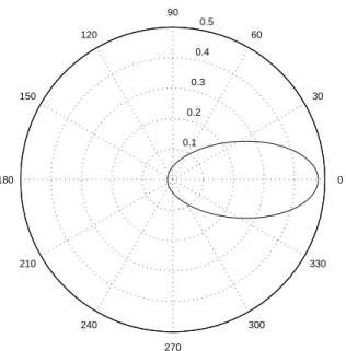
Figure 2.1: Plot of normalized Henyey-Greenstein phase function for g = 0.5.
weather conditions [Narasimhan and Nayar, 2003]. As an example, a polar plot of the Henyey-Greenstein phase function for g = 0.5 is shown in Figure 2.1
2.2
Light Scattering Terminology
This section lays out the groundwork and definitions used throughout this work.
2.2.1 Absorption, Emission, Scattering, and Extinction
The appearance of participating media is governed by the interaction of particles and light. Interactions include absorption, emission, scattering, and extinction.
Absorption
Absorption is the process when a particle absorbs some part of incident radiance. The
change of radiance L due to absorption at a point x in direction ω is given by
dL(x, ω)
where κa is the absorption coefficient.
Emission
Emission is the process when a particle converts some form of energy to emitted radiance.
The change of radiance L due to emission at a point x in direction ω is given by
dL(x, ω)
dx = Le(x, ω). (2.6)
Out-Scattering
Scattering is the process when a particle redirects (absorbs and re-emits) incident radiance to a new direction. Out-scattering refers to decreased radiance along a solid angle due to scattering outward into new directions. The change of radiance L due to out-scattering at a point x in direction ω is given by
dL(x, ω)
dx = −κsL(x, ω), (2.7)
where κs is the scattering coefficient.
In-scattering
In-scattering refers to increased radiance along a solid angle due to scattering from other
directions. Therefore, it must consider all incident radiance over the hemisphere of directions around a point x. The change of radiance L due to in-scattering at x in direction ω is given by dL(x, ω) dx = κs Z 4π p(ωi, ω)L(x, ωi)dωi. (2.8)
Scattering coefficient κsdetermines how much of incident radiance actually scatters at point x, whereas the phase function p(ωi, ω) determines how much of the scattered light redirects
towards direction ω. Extinction
Extinction, also known as attenuation, refers to the combined effect of absorption and
due to extinction at a point x in direction ω is given by
dL(x, ω)
dx = −κtL(x, ω). (2.9)
More Discussion
Alternatively, the coefficients κa, κs, and κt can be viewed as probability densities per unit distance that radiance is absorbed, scattered, or both. This means the coefficients may be any positive value, not necessarily between zero and one. These coefficients are properties of the density and mass of particles in the medium and in many cases, are spatially varying. In all encountered cases, these coefficients are a function of position, though strictly speaking, they could vary with direction. In purposes for computer graphics, it is sometimes convenient to assume uniform coefficients throughout a medium. Homogenous media are volumes with constant κt. Inhomogenous media are volumes with spatially varying κt.
2.2.2 Transmittance and Optical Thickness
If we consider a line segment from x0 to x, a solution to Equation 2.9 can be found, which is
L(x, ω) = L(x0, ω)e− Rx
x0κt(u)du= L(x0, ω)τ (x0, x). (2.10)
The solution describes the radiance at a new point x given an original point x0, with loss of radiance due to out-scattering and absorption.
Transmittance
Transmittance τ (x0, x) describes the fraction of radiance that is transmitted from point x0 to x along some path, where absorption and out-scattering account for the radiance reduction. As seen in the above equation, it is given by
τ (x0, x) = e− Rx
x0κt(u)du. (2.11)
An useful case is the assumption of a homogenous medium, where κt is constant.
Trans-mittance can easily be evaluated, yielding Beer’s Law:
where d is the distance from x0 to x. Optical Thickness
The exponent term −Rxx
0κt(u)du is known as optical thickness. Other names include optical
depth or optical length. On a side note, the symbols for optical thickness and transmittance
are sometimes identical in different works, though they represent different quantities. There is great potential for confusion since transmittance and optical thickness are closely related, though distinct, quantities. This is noted so as to avoid confusion on the part of the reader if cross-referencing.
2.3
Integral Transport Equation
The combination of all the processes described in Section 2.2.1 form the differential equation for light transport:
dL(x, ω) dx = κaLe(x, ω) + · κs Z 4π p(ωi, ω)L(x, ωi)dωi ¸ − κaL(x, ω) − κsL(x, ω). (2.13) Integrating both sides of the equation for a line segment from x0 to x yields the result:
L(x, ω) =
Z x
x0
τ (u, x)κa(u)Le(u, ω)du +
·Z x
x0
τ (u, x)κs(u)Li(u, ω)du
¸
+ τ (x0, x)L(x0, ω), (2.14) where Li(u, ω) is the in-scattered radiance at a point u. It is given by
Li(u, ω) = Z
4π
p(ωi, ω)L(u, ωi)dωi. (2.15)
The terms of Equation 2.14 correspond in order to the terms of the original differential form in Equation 2.13, with the exception that the last two terms of the differential form are combined into one before integration. This integral equation appears in various works in the literature on light transport and is mentioned here since the derivation from the differential form follows logically. In this work, however, we will refer more often to an alternative but equivalent form known as the integral transport equation, which is
L(x, ω) = τ (x0, x)L(x0, ω) + Z x
x0
where J(x, ω) is the source radiance that describes the local production of radiance. J(x, ω), which includes both self-emission and in-scattering, is given by
J(x, ω) = (1 − Ω(x))Le(x, ω) + Ω(x) Z
4π
p(ωi, ω)L(x, ωi)dωi, (2.17) where Ω = κs
κt is the albedo of the medium. The integral transport equation can be easier to
follow, especially when the source radiance term J(u, ω) simplifies easily under the common case when albedo is close to one. The relationship between the equivalent integral equations is shown below as a movement from Equation 2.16 to Equation 2.14:
L(x, ω) = τ (x0, x)L(x0, ω) + Z x
x0
τ (u, x)κt(u)J(u, ω)du
= τ (x0, x)L(x0, ω)+ Z x
x0
τ (u, x)κt(u) ·
(1 − Ω(u))Le(u, ω) + Ω(u) Z 4π p(ωi, ω)L(u, ωi)dωi ¸ du = τ (x0, x)L(x0, ω)+ Z x x0 τ (u, x)κt(u) · (κa(u) κt(u))Le(u, ω) + κs(u) κt(u) Z 4π p(ωi, ω)L(u, ωi)dωi ¸ du = τ (x0, x)L(x0, ω) + Z x x0
τ (u, x)κa(u)Le(u, ω)du + ·Z x
x0
τ (u, x)κs(u)Li(u, ω)du ¸
The challenge for rendering light scattering effects in computer graphics is developing models to solve the integral transport equation.
2.3.1 Simplifying Assumptions
Solving the integral transport equation(Equation 2.16) without making simplifying assump-tions is too complex for any practical rendering method. For atmospheric scattering, useful assumptions include homogeneous media, simple geometry, and large albedo close to one. For interactive methods, it is common to assume single scattering, which says that light scatters only once in the scene before reaching the viewer. There are widely varying models for multiple scattering, since the complexity for such models grows tremendously. Some models for multiple scattering will be presented in the Related Works of Chapter 3. For now, models for single scattering will be presented that exist throughout many works.
Point Light Source
The model for scattering from a point light source [Nishita et al., 1987] in a homogeneous medium is widely used in many rendering methods due to the simple form for transmittance in Equation 2.12. Under these assumptions, single-scattered radiance is given by
La= Z dvp 0 κtp(α) ·I0· e −κtd d2 · e−κtxdx (2.18)
The integral ranges from zero to the distance between viewer and nearest surface point,
dvp. The intensity of light reaching a scattering point along the view ray is I0·e−κtd d2 , since
I0 is the initial intensity of the point source, intensity is exponentially attenuated over the distance d, and intensity drops off by the inverse square law of distance. The intensity of light that reaches the view ray scatters by amount given by the extinction coefficient
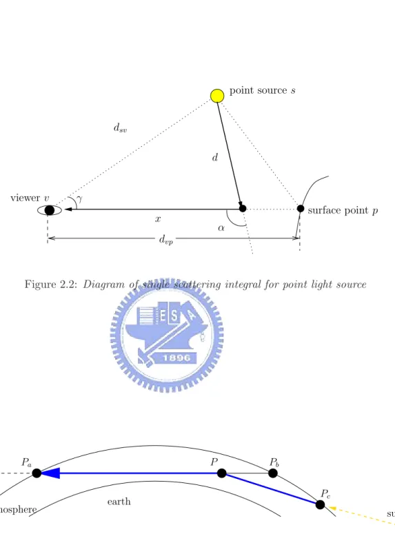
κt. The scattered light is redirected towards the viewer with frequency p(α). Finally, the remaining intensity is exponentially attenuated over distance x. A diagram is provided in Figure 2.2. Most single scattering methods for point light sources are slight variations of the above equation, such as angular intensity of the light source or visibility terms to consider volumetric shadows.
Single Scattering for Atmospheric Models
Sky and terrain rendering is a large area of research, whose origin largely traces to the single scattering model of [Nishita et al., 1993]. In this work, Rayleigh scattering with wavelength dependence is used, and the amount of scattering has exponential dependence on the height in the atmosphere, as an approximation to measurement analysis. Specifically, the atmospheric model for single-scattered radiance is
Iv = Is(λ)K(λ)p(α)
Z Pb
Pa
e−h/H0e−t(P Pc,λ)−t(P Pc,λ)ds, (2.19)
where optical depth t is
t(PaPb, λ) = K(λ)
Z Pb
Pa
e−h/H0ds. (2.20)
The equation integrates in-scattered radiance along the view ray from the nearest point in the atmosphere Pa to the farthest point in the atmosphere Pb, which may be the nearest
surface. In-scattered radiance enters the atmosphere at a point Pcand scatters at point P ,
as shown in Figure 2.3. Rayleigh scattering constant K(λ) has dependence on wavelength
λ, and the scattering coefficients e−h/H0 are exponentially dependent upon the height h
in the atmosphere. Constant H0 is associated with the height of the top of the atmo-sphere. Intensity from source Is(λ) may consider radiation other than white light. Phase
function p(α) depends on phase angle α, the angle between the directional source direction and the view ray. Many works build upon this model and include more complex effects such as halos, coronas, skylight, and sophisticated, precise measurements for atmospheric data [Nishita et al., 1996, Preetham et al., 1999, Riley et al., 2004].
dvp γ dsv surface point p point source s viewer v x α d
Figure 2.2: Diagram of single scattering integral for point light source
atmosphere
Pc
sunlight earth
Pa P Pb
Chapter 3
Related Work: Interactive
Rendering of Light Scattering
Effects
Creating realistic images of scenes with scattering media has long been an area of research within the computer graphics community due to the enhancement it lends to visual realism. The most complex effects of scattering to-date are captured using Monte Carlo ray tracing methods, including multiple scattering effects and non-homogeneous me-dia [Lafortune and Willems, 1996, Jensen and Christensen, 1998, Cerezo et al., 2005]. These methods, however, lack practicality for interactive applications because of the notoriously expensive procedures they require. Guided by the value to interactive applications, we describe in this chapter, therefore, representative methods for rendering of participating media towards interactive rates.
A thorough survey of works for rendering the effects of light scattering can be found in [Cerezo et al., 2005]. There are surveys with a narrower focus in atmospheric ren-dering [Preetham, 2003, Sloup, 2002]. With a focus on renren-dering techniques toward inter-active rates, the first subset of techniques for displaying scattering effects are characterized by solving the integral transport equation (Equation 2.16) using numerical methods, which we discuss in Section 3.1. Another set of works have explored the use of analytic techniques
for rendering participating media, which we discuss in Section 3.2. Before heading into a full-blown discussion on these sets of techniques, we first mention a small but significant observation that has guided this study: the proliferation of relevant works in recent years is owed not in small part to the acceleration and increased flexibility of commodity graph-ics hardware. The evolution of research in the field, thus, largely reflects these advances in hardware. This theme, though not explicitly mentioned, should run throughout the following chapter.
3.1
Numerical Methods
Unlike stochastic methods that may take hours to render a single image, many numerical solutions have been developed to accelerate the rendering process, though many still have limitations for real-time rendering applications. A common technique for numerical methods is to use two passes, the first for computing illumination within the medium and the second for rendering the medium.
3.1.1 Shafts of Light and Volumetric Shadows
Shafts of light result from the non-shadow regions of objects in participating media, whereas volumetric shadows result from the shadowed regions of objects in participating media. Illu-minated shafts of light were rendered interactively using virtual planes [Dobashi et al., 2000b], storing incident illumination on rectangular meshes lined up perpendicular to the view ray at regular intervals. The lighting equation used is Nishita’s single scattering integral for point light sources(Equation 2.18) with a visibility term added, seen here:
Ieye = Iobjβ(T ) +
Z T 0
F (α)H(t)Ip(t)β(t)dt. (3.1)
The notation is as follows: β(t) is the transmittance over distance t, T is the distance from the eye to the nearest object, F (α) is the phase function with phase angle α, H(t) is the visibility function(binary) of scattering point P , and Ip(t) is the intensity of light reaching P .
The key hardware acceleration was the storage of the F (α)Ip(t)β(t) term of the
perpendicular to the view ray at regular intervals. Storing the F (α)Ip(t)β(t) term requires
projecting a light map onto each ”virtual plane” to calculate part of Ip(t). Ignoring the
visibility term H(t) for a moment, the medium can then be rendered by
• sampling the integrand at lattice points of every virtual plane
• rendering the virtual planes with an additive blending function from back to front (volume rendering)
Only lattice points of the ”virtual planes” are used to sample the integrand to increase efficiency, and Gouraud interpolation is used to evaluate the term at any arbitrary point. The visibility term of the integrand, H(t), is applied by using the shadow map algorithm when rendering the virtual planes. That is, points on the virtual plane with depth value greater than the corresponding depth in the shadow map will have contribution zero when rendered. Banding problems caused by aliasing due to finite sampling limitations may occur in some situations. Increasing the amount of sampling is the straightforward solution; however, this quantity is highly dependent upon each scene and varies widely.
3.1.2 Atmospheric Effects
The method of [O’Neil, 2005] can render real-time atmospheric scenes either viewing the earth from space or the ground (like a horizon scene). Single-scattering approximations are adequate for these general atmospheric effects. Thus, this work essentially uniformly sam-ples the atmospheric model for single scattering of Equation 2.19 in the vertex or fragment shader using programmable graphics hardware. To evaluate optical depth terms, a polyno-mial best fit function was found using mathematical analysis software. Precomputed tables in texture memory may be used as well to compute optical depth terms, but polynomial functions were used to avoid texture lookups for hardware without texture lookup capabil-ity in the vertex shader. Furthermore, high dynamic range rendering is demonstrated for sky and terrain rendering. Since sampling is performed in the vertex or fragment shader, the cost of using a loop for sampling can dramatically increase if the scene requires greater accuracy. Otherwise, the method is effective for real-time rendering of atmospheric scenes with non-uniform scattering effects.
3.1.3 Multiple Scattering
Inhomogeneous media
By investigating the effects of multiple-scattering, Premoze et. al developed the point
spread function (PSF), which measures the spatial spreading of incident radiance in analytic
form [Premoze et al., 2004]. Based upon an analytic multiple scattering term derived from the point spread function, Hegeman et. al developed a lighting model for an inhomogeneous medium with multiple scattering effects at interactive rates [Hegeman et al., 2005], but illumination and medium parameters must be fixed. Other restrictions include the absence of volumetric shadows for objects within the medium. The lighting model uses both analytic and numerical techniques. Descriptions for the development of the point spread function, analytic multiple scattering term, and lighting model with multiple scattering effects follow. Using measurement analysis, Premoze et. al developed a point spread function that measures the spatial spreading of incident radiance for a given medium in an analytic form [Premoze et al., 2004]. Spatial spreading is described as the effect of a light beam’s broadening as it propagates through a medium. The point spread function has two param-eters, the amount of out-scattering l for a path and the distance S from the origin of the beam, and is given by
w2(l, S)d = < θ2 > lS2
24(1+ < θ2 > (a/b)l2/12, (3.2)
where a and b are the absorption and scattering coefficients, respectively, and < θ2 > is the mean square scattering angle. The work of [Premoze 2003] introduced the notion of a Most Probable Path (MPP), such that only paths close to MPPs contribute to a mul-tiple scattering contribution. Also, an alternative method for modeling light scattering is introduced, known as the path integral. The path integral formulation describes an integral over an infinite number of possible paths, for which only out-scattering need be accounted. Using both the path integral formulation and point spread function, an analytic term for multiple scattering contribution in a strongly forward-scattering inhomogeneous medium is developed. It is based upon the assumption that only paths close to the MPP are added to the contribution. Additionally, curved MPPs are approximated by two linear segments.
The result for the multiple-scattering contribution is LM S(x, ω) = Z l dl×e−(c/b)l(M P Ple−Ac(M P Pl)×P M S(l, ω−ω0) Z plane gauss(x0, w(l))L0(x0, ω0)dx0 (3.3) The outer integral is an integral over MPPs, each with scattering parameter l. The inner integration is the gaussian-weighted incident radiance in the plane perpendicular to the light direction. c is the extinction coefficient. Ac is a curvature term. PM S is a multiple
scattering phase function.
Based upon the above multiple scattering term, Hegeman et. al developed a lighting model for an inhomogeneous medium with multiple scattering effects at interactive rates [Hegeman et al., 2005]. The scene is restricted to static directional light and a static volume. Strongly forward-scattering with mean square scattering angle < θ >2is reasonably assumed. The main contribution of this work was the implementation of the multiple scattering term using graphics hardware and data structures for acceleration. To accomplish this task, a couple of large data structures are created before rendering. A 3D precomputed light volume data structure stored an approximation for the total radiance arriving at each voxel, essentially computing the scattering parameter l of Equation 3.3. A second data structure for accelerated performance, called the LightImage, is a visibility map from the perspective of the volume. A mipmap pyramid is constructed where each level blurs over a different width w. The LightImage essentially computes the inner integral of Equation 3.3. With these data structures, a technique of volume rendering can be applied to render the medium, effectively sampling the integral for paths close to the view ray. A series of view-aligned planes, whose vertices are assigned texture coordinates corresponding to their intersection with the light volume at regular intervals, are created for each frame and rendered in back-to-front order with an additive blending function.
Cloud Rendering
Based on a two-pass rendering technique employed by [Dobashi et al., 2000a] for clouds under a single scattering assumption, a complete system for real-time cloud rendering [Harris and Lastra, 2001] was developed that used a particle system to model clouds and
precomputed an isotropic multiple forward scattering term in dynamically-generated im-postors during an initial illumination pass. Anisotropic single scattering was accounted for during the second visualization pass. To amortize the cost over many frames, impostors are required to achieve real-time rates. Evaluation of the differential form (Equation 2.13) for the integral light transport equation is done as a recursive operation, where each step attenuates the old radiance and adds the source radiance contribution of the present parti-cle from back to front. The partiparti-cles are rendered using splatting, such that the partiparti-cles are sorted with respect to the light and rendered back-to-front with a recursive blending equation. The method is specifically tailored to scattering seen in clouds. Another limiting factor is the precomputation required, which is dependent upon the scene illumination and scattering properties.
3.2
Analytic Methods
Analytic methods significantly improve the performance for rendering of scenes with par-ticipating media. Their major drawback lies in the increased number of assumptions and simplifications made for the sake of performance.
3.2.1 Effects for Point Light Sources
Assuming point light sources simplifies computation but can be effective for scenes in which the source is inside the participating medium, creating effects of glows around light sources. Complex effects such as multiple scattering for glows and scattering effects on surface radi-ance can be realized.
Multiple Scattering
The work of [Narasimhan and Nayar, 2003] modeled multiple scattering from an isotropic point light source using an analytic expression termed the atmospheric point spread function. Assumptions include homogeneous media, infinite extent, and distant light sources. There-fore, it neglects effects on surface radiance. Using an expansion of the Henyey-Greenstein phase function as a series Legendre polynomials, a series solution to the integral transport
equation (Equation 2.16) is derived, assuming homogeneous media and distant point light sources. The work shows that the shape of the point spread function largely depends on the atmospheric conditions, the source intensity, and the depth of the source. An analysis of glows under different weather conditions is described, including rendered images. Volumetric Shadows
In [Biri et al., 2006], the authors developed an analytic expression for the single scattering integral for point light sources in a homogeneous medium using a polynomial approxima-tion that can be implemented on graphics hardware. The polynomial approximaapproxima-tion is obtained by first using an angular reformation of the single scattering integral for point light sources [Lecocq et al., 2000], which is described in a later chapter (Equation 4.3). Then the integral is approximated as a polynomial of a single angle with degree four. The constants of the polynomial are determined by the type of scattering chosen. Unfortunately, inaccurate glows appear when the viewer is near the source. Also, no effects on surface radi-ance are considered. An algorithm for incorporating volumetric shadows is also introduced. The basic concept is that the scattering contribution of non-shadowed regions may be ren-dered by subtracting the contribution of shadowed regions, whose equivalent is rendering the shadow volume using an analytic scattering contribution. There is an exception–shadow polygons which are themselves in shadow should not be rendered. The algorithm essentially constructs a standard shadow volume, sorts shadow polygons according to their estimated depths, and then renders the shadow polygons using a positive scattering contribution for back-facing shadow polygons and a negative scattering contribution for front-facing shadow polygons. Limitations occur when the estimated depths of large polygons have errors. Scattering Effects on Surface Shading and Environment Map Lighting
The work of [Sun et al., 2005] developed a real-time analytic single scattering model for point light sources that can render visual effects on surface shading and handle complex environment map lighting using programmable graphics hardware. Significant effects such as glows around light sources, spreading of specular highlight on objects, and brightening of shadows were realized in real-time fog scenes. The effects of anisotropic scattering, though
considered in the model, were not demonstrated. The inclusion of anisotropic scattering in the model induces a loss in both performance and accuracy.
Visual results of glows and scattering effects on surface shading were realized in real-time, a difficult task due to the complexity of volumetric scattering for all surface points. Analytic evaluation of the single scattering integral for point light sources
[Nishita et al., 1987] was made possible by changing the variables of integration and deriving a form that could be largely precomputed into a table. Complex integrals are expressed as 2D functions that can be precomputed into tables and placed in texture memory. The functions then can be accurately evaluated at run-time using texture lookups with linear interpolation. With this technique, an analytic model for scattering contribution to surface radiance is developed, under the assumption that no objects are in the path of scattered light.
Complex brdf and environment map lighting under foggy conditions is also pre-sented, enabling environment maps to include effects of glows around light sources as well as enabling precomputed radiance transfer methods to incorporate scattering effects. By fit-ting empirical data, the work develops an analytic point spread function of a single angular parameter that can be convolved with an environment map to produce a new environ-ment map which exhibits glows around light sources. This technique can be applied on the environment lighting used in precomputed radiance transfer methods as well.
3.2.2 Sky and Terrain Rendering
The rendering of scenes with both sky and terrain requires models for sky and aerial per-spective. Sky models only describe the illumination of skylight, whereas aerial perspec-tive models describe the in-scattering of skylight and out-scattering that occurs before it reaches the viewer. Consequently, aerial perspective models must consider the position of the viewer and usually requires larger amounts of computation. Significantly more effi-cient and practical than their numerically-simulated counterparts, complex analytic models that fit measured atmospheric data have been developed that exhibit angular dependent and multiple scattering effects [Preetham et al., 1999, Riley et al., 2004]. The utilization of graphics hardware is used in some cases; however, these methods are still far from
interac-tive.
The work of [Hoffman and Preetham, 2003] can render skies using programmable graphics hardware in the vertex or fragment shader in real-time. A simple, analytic form for scattering from a directional light source is made possible when a constant density atmosphere is assumed, thus assuming constant scattering as well. Under this assumption, the scattering coefficient can be expressed as Rayleigh and Mie scattering constants with dependence on wavelength. The result for atmospheric scattering is the lighting equation:
L(s, θ) = L0e−(κs,R+κs,M)s+κs,RpRκ(θ) + κs,MpM(θ)
s,R+ κs,M Esun(1 − e
−(κs,R+κs,M)), (3.4)
where κs,R and κs,M are the Rayleigh and Mie scattering coefficients, respectively. pR(θ)
and pM(θ) are the Rayleigh and Mie phase functions, respectively(Equations 2.2 and 4.1). The scattering coefficient(κs) is split into the sum of its parts (κs= κs,R+κs,M). Rendering
a sky thus equates to rendering a tessellated sky dome with implementation of Equation 3.4 in the vertex or fragment shader.
Chapter 4
Analytic Lighting Model for
Accurate and Dynamic Anisotropic
Scattering
Reiterating earlier goals, our objective is to develop a practical rendering method for real-time graphics applications that considers increasingly complex scattering effects and dynamic behavior. Under this premise, we develop a lighting model for atmospheric environments such as fog, mist, or haze that allows users to create and adjust scattering conditions interactively using simple parameters. This type of interactive capability enables what is heretofore referred to as a dynamic scattering environment, where the medium’s level of forward scattering and density may be changed in real-time.
For most atmospheric conditions, a phase function p(θ) symmetric about the in-cident direction is sufficient to describe a scattering distribution [Cerezo et al., 2005]. The Henyey-Greenstein phase function [Ishimaru, 1997] is widely used in computer graphics for its relative simplicity and effectiveness for common atmospheric environments. Its normal-ized form is repeated here for easy reference:
p(θ) = 1 − g2
4π(1 + g2− 2g cos θ)3/2, (4.1)
Values g > 0 correspond to forward scattering, g = 0 corresponds to isotropic scattering, and g < 0 correspond to backward scattering. Positive values for g can describe most weather conditions [Narasimhan and Nayar, 2003]. By varying forward scattering param-eter g, different scattering conditions can be modeled. The presented lighting model can demonstrate complex visual affects of glows around light sources and effects on surface ra-diance under varying scattering conditions. These findings are described in a later chapter describing results in Section 5.1.
In this chapter, we present our analytic lighting model with an extension for a dynamic scattering environment that all may be implemented on programmable graphics hardware in real-time. The basic underlying strategy for analytic evaluation of scattering integrals is the use of precomputed two-dimensional tables. By converting the scattering integrals into forms that may be expressed as functions of two parameters, the functions may then be precomputed as two-dimensional tables and placed in the texture memory of graphics hardware. Using programmable graphics hardware, the functions may be evaluated with a simple texture lookup in the vertex or fragment shader.
This chapter is divided into four sections: an introduction section, a detailed description of the proposed analytic lighting model, an extension to the analytic model for dynamic anisotropic scattering, and lastly, a description of the hardware implementation.
4.1
Introduction
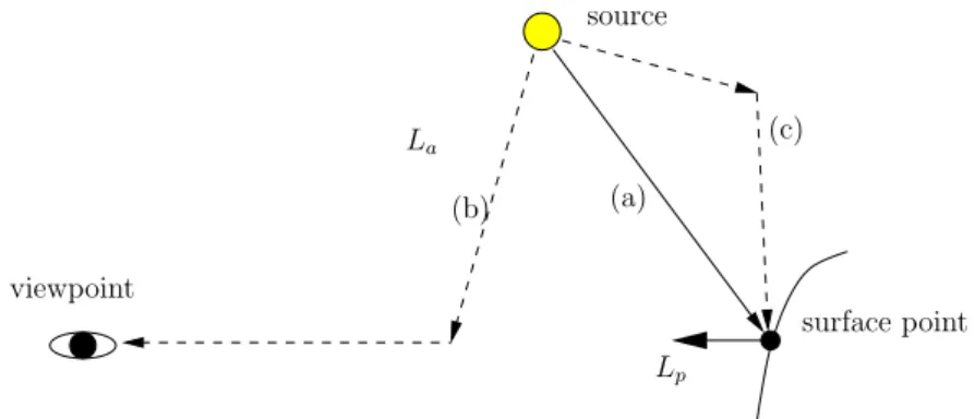
Let us consider the paths of light transport for single scattering depicted in Figure 4.1. Light rays may (a) directly transmit through the medium, leading to attenuation; (b) scatter once from source to viewer, leading to glows around sources [Narasimhan and Nayar, 2003]; or (c) scatter once from source to surface point, leading to diffusing of reflected surface radiance and brightening of shadows [Sun et al., 2005]. The aforementioned paths and their visual effects can be captured by the sum of reflected surface radiance Lp with attenuation and airlight from source to viewer La [Sun et al., 2005]:
L = e−κtdvpL
surface point source viewpoint (a) (c) Lp (b) La
Figure 4.1: Diagram illustrating light paths of (a) direct transmission, (b) airlight from
source to viewer, and (c) airlight from source to surface point. Path (b) contributes to airlight from source to viewer La. Paths (a) and (c) contribute to reflected surface radiance
Lp.
where κt is the extinction coefficient of the participating medium and dvp is the distance
between the viewpoint and surface point. Subsequent sections develop a solution to this lighting equation.
4.2
Analytic Lighting Model
In this section, we develop analytic models to compute airlight La, which is responsible for
glows around light sources, in Section 4.2.1 and surface radiance Lp, which is affected by airlight from source to surfaces, in Section 4.2.2. Lastly, a summary of the analytic lighting model is provided in Section 4.2.3
4.2.1
Angle-Formulated Airlight Model
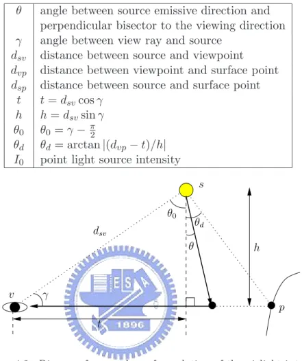
The contribution of airlight depicted as path b in Figure 4.1 is given by the classic integral along the viewing direction for single-scattered airlight from an isotropic point light source [Nishita et al., 1987], which is expressed in terms of the distance along the ray. To reduce the number of physical parameters in the integral, we introduce the angle reformulation of the single scattering integral for airlight from a point light source [Lecocq et al., 2000]:
La(γ, dsv, dvp, κt) = κtI0e−κtt h Z θ d θ0 e−κth(sin θ+1cos θ )p(θ + π 2)dθ. (4.3)
Table 4.1: Notation and formulae for angle-formulated airlight integral.
θ angle between source emissive direction and perpendicular bisector to the viewing direction γ angle between view ray and source
dsv distance between source and viewpoint
dvp distance between viewpoint and surface point
dsp distance between source and surface point
t t = dsvcos γ
h h = dsvsin γ
θ0 θ0= γ − π2
θd θd = arctan |(dvp− t)/h|
I0 point light source intensity
dsv v γ θd p t s h θ θ0
Figure 4.2: Diagram for angular reformulation of the airlight integral.
The integral is expressed in terms of the angle θ between the light source emissive direction and the perpendicular bisector to the viewing direction with respect to s, as depicted in Figure 4.2. θd and θ0 are the bounds of integration. See [Biri et al., 2006] for a derivation of the angle reformulation. Refer to Table 4.1 for the rest of the notation. We refer to Equation 4.3 in the remainder of the paper as the angle-formulated airlight integral.
Analytic solution to Airlight La
To solve Equation 4.3, it is factorized into an analytic expression dependent on the physical parameters of the scene and a tabulated function independent of the physical parameters. Let C0(γ, dsv, κt) = κtI0e−κtt/h, (4.4) C1(γ, dsv, κt) = κth. (4.5) Then La= C0 Z θd θ0 e−C1(sin θ+1cos θ )p(θ + π 2)dθ.
The angle-formulated airlight integral now is factorized into an analytic expression C0 and an integral that may be expressed as a function of two variables. The result for an analytic solution to Equation 4.3 is La= C0[H(C1, θd) − H(C1, θ0)]. (4.6) where H(u, v) = Z v −π 2
e−u(sin θ+1cos θ )p(θ +π
2)dθ. (4.7)
As a function independent of the physical parameters of the scene, H(u, v) can be nu-merically integrated during the precomputation stage into a table and stored into texture memory. The plot of H(u, v) in the isotropic scattering case p(θ) = 4π1 is shown in Fig-ure 4.3, demonstrating that the function is smooth. Thus, the tabulated function H(u, v) in texture memory can be accessed during run-time using linear interpolation for evaluation of the integral. It is worth mentioning that any phase function p(θ) may be used in our lighting model without significantly affecting run-time performance or accuracy, thus mak-ing it general for any type of anisotropic scattermak-ing. Airlight from a point source may be computed with just evaluation of analytic functions and two texture lookups in the vertex or fragment shader using programmable graphics hardware. The choice of p(θ) does not affect run-time performance since H(u, v) is constructed in a precomputation stage. The special case of no objects along the view ray (dvp = ∞, θd = π2) is important for the next
−1.5 −1 −0.5 0 0.5 1 1.5 0 2 4 6 8 10 0 0.05 0.1 0.15 0.2 0.25 v u H
Figure 4.3: 3D plot of function H(u, v) for u ∈ [0, 10] and v ∈ [−π/2, π/2] for p(θ) = 1/(4π). The graph demonstrates that the function is smooth, thus making it appropriate for
tabulation during precomputation and look-up during run-time.
subsection. In such a case, the airlight is
La(γ, dsp, ∞, κt) = C0[H(C1,π
2) − H(C1, θ0)]. (4.8)
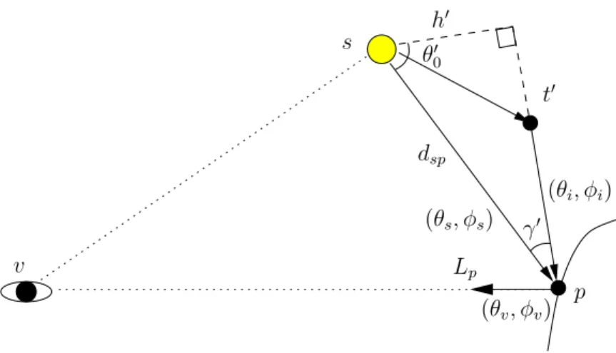
4.2.2 Surface Radiance Model using Angle Formulation
Reflected radiance Lp is the sum of contribution from direct transmission Lp,d (path a in
Figure 4.1) and contribution from airlight Lp,a (path c in Figure 4.1), which is given by the
surface radiance single scattering integral [Sun et al., 2005]. This is written as
Lp = Lp,d+ Lp,a, (4.9) where Lp,d =I0e−κtdsp dsp2 BRDF (θs, φs, θv, φv) cos θs, (4.10) Lp,a= Z Ω2π La(γ0, dsp, ∞, κt)BRDF (θi, φi, θv, φv) cos θidωi. (4.11)
γ0 v p dsp (θi, φi) (θs, φs) Lp s (θv, φv) h0 θ0 0 t0
Figure 4.4: Diagram for light paths of direct transmission and airlight to surface point that
contribute to surface radiance Lp.
The surface radiance single scattering integral sums airlight contribution to surface radiance over the surface point’s hemisphere of incident directions. The angle γ0 is the angle between the source direction (θs, φs) and incident direction (θi, φi), such that h0 = dspsin γ0 and t0 = dspcos γ0. Refer to Figure 4.4 for a depiction of the these variables. To simplify the
integral for evaluation, the airlight term La in Equation 4.11 assumes no object obstructs
each incident direction(dvp= ∞,θd= π2).
Analytic solution to Surface Radiance Lp
We solve Lp for both the Lambertian BRDF and Phong BRDF separately. For the
Lam-bertian case, BRDFLam= kd, where kdis the diffuse constant of the object. For the Phong
case, all angles of Equation 4.9 are reparameterized against the reflection of the view ray about the surface normal [Ramamoorthi and Hanrahan, 2002] to reduce the complexity of the integral. We denote the reparameterizated source direction θ0
s. After
reparameteriza-tion, BRDFP hong = kscosnθ0i, where ksis the specular constant of the object. The resultant
solution for Lp,d is straightforward:
Lp,d = I0e−κtdsp
dsp2
(kdcos θs+ kscosnθs0). (4.12)
To solve Lp,a, we make the substitution Tsp= κtdsp and use our analytic model for airlight La, Equation 4.8. Other substitutions and simplifications are made, allowing us to
re-express the integral portion as a function of two parameters. The details of this derivation for the solution to Lp,a are shown below:
Lambertian BRDF case:
Lp,a= Z
Ω2π
La(γ0, dsp, ∞, κt)BRDF (θi, φi, θv, φv) cos θidωi
1. Substitute La(γ0, dsp, ∞, κt) with Equation 4.8 and BRDF (θi, φi, θv, φv) with kd.
= Z
Ω2π
C0(γ0, dsp, κt)[H(C1(γ0, dsp, κt),2π) − H(C1(γ0, dsp, κt), θ00)]kdcos θidωi
2. Substitute for C0(γ0, dsp, κt), C1(γ0, dsp, κt), θ00, and Tsp = κtdsp.
3. Take constants out of integral. = I0kdκt dsp Z Ω2π e−Tspcos γ0 sin γ0 [H(Tspsin γ0, π 2) − H(Tspsin γ 0, γ0−π 2)] cos θidωi 4. Recall γ0(θs, ωi). So = I0kdκt dsp J 1(T sp, θs) where J1(Tsp, θs) = Z Ω2π e−Tspcos γ0 sin γ0 [H(Tspsin γ 0,π 2) − H(Tspsin γ 0, γ0−π 2)] cos θidωi. (4.13)
Phong BRDF case:
Lp,a=
Z Ω2π
La(γ0, dsp, ∞, κt)BRDF (θi, φi, θv, φv) cos θidωi
1. Let R be the reflection of the view ray about the surface normal. 2. Reparameterize the integral about R.
3. Denote reparameterized source direction θs0[s.t. γ0(θs0, ωi) and θ00(θs0, ωi)].
4. Substitute La(γ0, dsp, ∞, κt) = Equation 4.8 and BRDF (θi, φi, θv, φv) = kscosnθ0i.
= Z
Ω2π
C0(γ0, dsp, κt)[H(C1(γ0, dsp, κt),π2) − H(C1(γ0, dsp, κt), θ00)]kscosnθidωi
5. Substitute for C0(γ0, dsp, κt), C1(γ0, dsp, κt), θ00, and Tsp = κtdsp.
6. Take constants out of integral. = I0ksκt dsp Z Ω2π e−Tspcos γ0 sin γ0 [H(Tspsin γ0, π 2) − H(Tspsin γ 0, γ0−π 2)] cos nθ idωi = I0ksκt dsp J n(T sp, θ0s) where Jn(Tsp, θs0) = Z Ω2π e−Tspcos γ0 sin γ0 [H(Tspsin γ0, π 2) − H(Tspsin γ 0, γ0− π 2)] cos nθ idωi. (4.14)
The resultant solution for Lp,ais
Lp,a= I0κt dsp
[kdJ1(Tsp, θs) + ksJn(Tsp, θ0s)], (4.15)
Both J1(T
sp, θs) and Jn(Tsp, θ0s) can be numerically integrated, tabulated, and stored into
texture memory during a precomputation stage, where n denotes the Phong exponent. Consequently, each of these functions can be evaluated with a texture lookup using linear interpolation during run-time. Plots of J1 and Jn (n = 20) are shown in Figure 4.5, demonstrating that they are smooth.
0 0.5 1 1.5 0 2 4 6 8 10 0 0.2 0.4 0.6 0.8
T
sp
θ
s
J
1
(a) 0 0.5 1 1.5 0 2 4 6 8 10 0 0.1 0.2 0.3 0.4T
sp
θ
s
′
J
2
0
(b) Figure 4.5: 3D plots of functions (a) J1(Tsp, θs) and (b) J20(Tsp, θ0s) for Tsp ∈ [0, 10] and
θs ∈ [0, π/2]. The graphs demonstrate that the functions are smooth, thus making them
4.2.3 Summary of Analytic Lighting Model
In this section, a full analytic solution to lighting equation 4.2 is developed. The model can capture visual effects for glows around light sources and on surface radiance. Additionally, it may consider any anisotropic scattering distribution described by a phase function of one parameter under the assumption of single scattering. The complexity of the phase function has no effect on run-time performance whatsoever, since its computation is isolated to a precomputation stage. An illustrative summary of the analytic lighting model presented thus far is shown in Figure 4.6.
The choice of phase function p(θ) greatly affects the visual appearance of partici-pating media, since it indicates different scattering conditions. The lighting model discussed up to this point requires the phase function p(θ) to be predetermined, as is common in many scattering models. Without instant visual feedback, it is often cumbersome to manipulate
p(θ) to achieve desirable visual results. Furthermore, only a pre-determined, limited
num-ber of scattering environments are possible for interactive applications with this restriction. In the next section, we develop an extension to our lighting model, allowing the user to change the level of forward scattering in real-time.
viewpoint
source
Lp
surface point
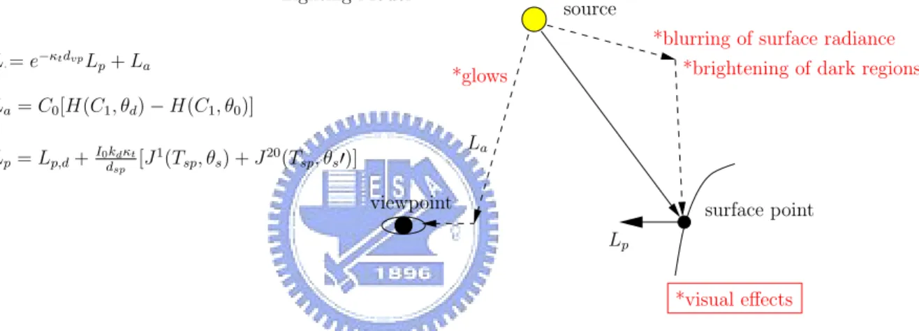
*glows
*blurring of surface radiance *brightening of dark regions
La Lighting Model *visual effects L = e−κtdvpL p+ La Lp= Lp,d+I0dkspdκt[J1(Tsp, θs) + J20(Tsp, θs0)] La= C0[H(C1, θd) − H(C1, θ0)]
Figure 4.6: Illustrative summary of analytic lighting model in Section 4.2. L is implemented
in the vertex or fragment shader using programmable graphics hardware. Each evaluation of function H, J1, or J20 costs a single texture lookup.
4.3
Dynamic Anisotropic Scattering
In this section, an extension to the analytic model of Section 4.2 for dynamic forward scat-tering is presented. Many previous works must use a pre-determined phase function before run-time, making it difficult to pre-visualize different scattering conditions and limiting the number of scattering environments possible for interactive applications. With the capabil-ity of manipulating the phase function at run-time, instant visual feedback as well as an unlimited variation of scattering environments is possible.
The form of the Henyey-Greenstein phase function in Equation 4.1 hinders inter-active modification of scattering parameter g. We use a well known fact in the literature on light transport that phase functions can be written as a series of Legendre polynomials [Dunn, 1997, Narasimhan and Nayar, 2003]:
p(cos θ) = 1 4π N X k=0 (2k + 1)bkPk(cos θ), (4.16)
where Pk(cos θ) is the Legendre polynomial of order k. The first four Legendre polynomials are listed below:
P0(x) = 1 P1(x) = x P2(x) = 1 2(3x 2− 1) P3(x) = 12(5x3− 3x)
In the case of the Henyey-Greenstein phase function, the expansion coefficients are bk= gk.
Using this alternative expression for the Henyey-Greenstein phase function, we can develop analytic solutions to airlight La (Equation 4.3) and surface radiance Lp
(Equa-tion 4.9) with dynamic scattering by using the Legendre expansion, Equa(Equa-tion 4.16, for p(θ) and moving forward scattering parameter g outside of any precomputed integrals. These steps are shown as follows:
![Figure 4.3: 3D plot of function H(u, v) for u ∈ [0, 10] and v ∈ [−π/2, π/2] for p(θ) = 1/(4π)](https://thumb-ap.123doks.com/thumbv2/9libinfo/8756439.207010/40.892.193.793.180.765/figure-d-plot-function-h-π-π-θ.webp)
![Figure 4.5: 3D plots of functions (a) J 1 (T sp , θ s ) and (b) J 20 (T sp , θ 0 s ) for T sp ∈ [0, 10] and θ s ∈ [0, π/2]](https://thumb-ap.123doks.com/thumbv2/9libinfo/8756439.207010/44.892.261.703.217.947/figure-plots-functions-t-t-sp-θ-π.webp)