用於混合式耐延遲網路之適地性服務資料搜尋方法 - 政大學術集成

全文

(1)國立政治大學資訊科學系 Department of Computer Science National Chengchi University . 碩士論文 Master’s Thesis. 立. . 政治大. ‧. ‧ 國. 學. 用於混合式耐延遲網路之適地性服務資料搜尋方法 Location-based Content Search Approach in Hybrid Delay Tolerant Networks n. engchi. er. io. Ch. sit. y. Nat. al. . i Un. v. 研究生：李欣諦指導教授：蔡子傑 . 中華民國一零一年七月 July 2012 .

(2) 用於混合式耐延遲網路之適地性服務資料搜尋方法 Location-based Content Search Approach in Hybrid Delay Tolerant Networks 研究生：李欣諦. Student：Hsin-Ti Lee. 指導教授：蔡子傑. Advisor：Tzu-Chieh Tsai. 大學 ‧. ‧ 國. 立. 政治國立政治大學資訊科學系碩士論文. n. er. io. sit. y. Nat. A Thesis submitted to Department of Computer Science National Chengchi University in partialafulfillment of the Requirements iv l C n forhthe e ndegree g c h iofU Master in Computer Science. 中華民國一零一年七月 July 2012. .

(3) 用於混合式耐延遲網路之適地性服務資料搜尋方法. 摘要. 在耐延遲網路上，離線的使用者，可以透過節點的相遇，以點對點之特定訊息繞送方法，將資訊傳遞至目的地。如此解決了使用者暫時無法上網時欲傳遞資訊之困難。因此，在本研究中，當使用者在某. 政治大. 一地區，欲查詢該地區相關之資訊，但又一時無法連上網際網路時，. 立. ‧ 國. 學. 則可透過耐延遲網路之特性，尋求其它同樣使用本服務之使用者幫忙以達到查詢之目的。. ‧. 本論文提出一適地性服務之資料搜尋方法，以三層式區域概念，. sit. y. Nat. 及混合式節點型態，並透過資料訊息複製、查詢訊息複製、資料回覆. er. io. n. al 及資料同步等四項策略來達成使用者查詢之目的。特別在訊息傳遞方 iv Ch. n engchi U. 面，提出一訊息佇列選擇演算法，賦予優先權概念於每一訊息中，使得較為重要之訊息得以優先傳送，藉此提高查詢之成功率及減少查詢之延遲時間。最後，我們將本論文方法與其它查詢方法比較評估效能，其模擬結果顯示我們提出的方法有較優的查詢效率與延遲。. 關鍵字：耐延遲網路、適地性服務、內容、查詢、路由協定. i .

(4) Location-based Content Search Approach in Hybrid Delay Tolerant Networks Abstract In Delay Tolerant Networks (DTNs), the offline users can, through the encountering nodes, use the specific peer-to-peer message routing approach to deliver messages to the destination. Thus, it solves the problem that users have the demands to deliver messages while they are. 政治大. temporarily not able to connect to Internet. Therefore, by the. 立. characteristics of DTNs, people who are not online can still query some. ‧ 國. 學. location based information, with the help of users using the same service in the nearby area.. ‧. In this thesis, we proposed a Location-based content search approach.. y. Nat. io. sit. Based on the concept of three-tier area and hybrid node types, we. er. presented four strategies to solve the query problem. They are Data. n. a. v. l C Data Reply and Replication, Query Replication, n i Data synchronization. hengchi U. strategies. Especially in message transferring, we proposed a Message Queue Selection algorithm. We set the priority concept to every message such that the most important one could be sent first. In this way, it can increase the query success ratio and reduce the query delay time. Finally, we evaluated our approach, and compared with other routing schemes. The simulation results showed that our proposed approach had better query efficiency and shorter delay. Keywords: Delay Tolerant Networks, Location-based, Content, Query, Routing protocol ii .

(5) 致謝辭. 研究所這兩年，時間不長也不短，但學習到的事物卻相當的有份量。過去是資訊管理系的我，鼓足勇氣，一腳踏入資訊科學領域，這過程相當感謝許多人的指導以及提攜，時常聽人說，讀研究所是為了提升自己獨立解決問題的能力，而在政大資科所的這兩年訓練想必也有所成長。能夠完成這份論文，最要感謝指導教授蔡子傑老師的細心教導，讓我能順利的從一開始的發想到確定方向，進而一步一步的完成碩士論文，在每一次的討論，. 政治大不迷失方向，使得能如此順利的完成碩士論文，由衷的感謝蔡子傑老師的提攜及立老師都能精闢點出問題所在，並給予受用的回饋，讓我在研究過程中有所指引而. ‧ 國. 學. 指導。. 而接著我要感謝幫助我能快速的瞭解實驗室研究及相關生活問題解答的學. ‧. 長姐，文卿、勇麟、偉敦、凱禎、彥嵩、賀翔，其中要感謝即時雨勇麟學長，在. sit. y. Nat. 我剛進入政大，還在為生活費苦惱時，即時的提供了英文系工讀的機會，讓我能. n. al. er. io. 在研究所這兩年間不需煩惱生活費問題，而同時也感謝我的同學們，英明、昶瑞、. i Un. v. 冠傑、郁翔在修課及研究上能互相討論及幫忙，另外也謝謝學弟們，煜泓、宇軒、. Ch. engchi. 建淳在校慶軟體開發時的幫忙，才能順利的完成老師的各項需求，此外，我要感謝我的好朋友舜然，在辛苦上班結束後還能播空陪我一起玩遊戲舒解壓力，在我煩悶的研究生活中，讓我能在撰寫論文時繃緊的神經能有所放鬆。最後祝福各位在未來不論是工作或求學期間都能夠事事順心、健康快樂。最後我要感謝我的家人，在我逆境時能給予最大的支持及鼓勵，讓我能一次又一次的突破困境，一路讀到了碩士，進而取得學位，沒有你們，我的求學之路不會如此順遂，謝謝你們。. iii .

(6) TABLE OF CONTENT CHAPTER 1 Introduction ..........................................................................1 1.1 Background ....................................................................................1 1.2 Motivation ......................................................................................2 1.3 Objective ........................................................................................3 1.3.1 Replication issues .................................................................4 1.3.2 Data Reply issue...................................................................4. 政治大. 1.3.3 Data Synchronize issue ........................................................5. 立. 1.4 Organization ...................................................................................5. ‧ 國. 學. CHAPTER 2 Related Work ........................................................................6 2.1 Common DTN routing protocol ....................................................6. ‧. 2.1.1 Flooding-based routing schemes..........................................6. y. Nat. io. sit. 2.1.2 Forwarding-based routing schemes .....................................8. er. 2.2 Query-based DTN routing protocol ...............................................8. n. a. v. l C 2.2.1 Locus: A Location-based Data Overlay n i for. hengchi U. Disruption-tolerant Networks [11] ................................................9 2.2.2 Performance Evaluations of Data-centric Information Retrieval Schemes for DTNs [12]...............................................10 2.2.3 Cooperative File Sharing in Hybrid Delay Tolerant Networks [13] ............................................................................. 11 2.2.4 Searching for Content in Mobile DTNs [14] .....................12 CHAPTER 3 Location-Based Content Search Approach ........................13 3.1 Data replication strategic .............................................................20 3.2 Query replication strategic ...........................................................22 iv .

(7) 3.3 Data Reply strategic .....................................................................25 3.4 Data synchronization and update strategic ..................................28 3.5 Message queue selection algorithm .............................................29 CHAPTER 4 Simulation Results ..............................................................31 4.1 Simulation Setup ..........................................................................32 4.2 Simulation Settings ......................................................................33 4.3 Simulation Results .......................................................................34 4.3.1 The percentage of node type ..............................................34 4.3.2 Radius of Inside Area .........................................................37. 治政大 4.3.3 Node Density...................................................................... 39 立 4.3.4 Buffer Size .........................................................................43. ‧ 國. 學. 4.3.4 Time to Live .......................................................................45. ‧. CHAPTER 5 Conclusions and Future Work ............................................48. n. al. er. io. sit. y. Nat. REFERENCE............................................................................................49. Ch. engchi. v . i Un. v.

(8) LIST OF FIGURE Figure 1: Problem scenario ................................................................. 3 Figure 2: Locus approach [11] .......................................................... 10 Figure 3: Hybrid DTN example [13] ................................................. 11 Figure 4: Database Tables ...................................................................14 Figure 5: three parts area figure ........................................................ 15 Figure 6: LCS workflow ................................................................... 18 . 政治大 Figure 8: Data replication 立 strategic flow chart .................................. 22 . Figure 7: LCS transmission protocol ................................................. 19 . ‧ 國. 學. Figure 9: Query replication strategic flow chart ................................ 24 Figure 10: Moving direction and the relative distance ...................... 27 . ‧. Figure 11: Data reply strategic flow chart ......................................... 27 . sit. y. Nat. Figure 12: Data sync and update strategic flow chart ........................ 28 . er. io. Figure 13: Message Queue Selection ................................................ 29 . n. al Figure 14: Map of Taipei101 surrounding area ................................. 32 iv Un. C. hengchi Figure 15: ONE simulator ................................................................. 33 Figure 16: Query-Reply Success Ratio (Node Type) ........................ 35 Figure 17: Query Delivery Ratio (Node Type) .................................. 35 Figure 18: Overhead (Node Type) ..................................................... 36 . Figure 19: Latency (Node Type) ....................................................... 36 Figure 20: Query-Reply Success Ratio (Radius of Inside Area) ....... 37 Figure 21: Overhead (Radius of Inside Area) .................................... 38 Figure 22: Latency (Radius of Inside Area) ...................................... 38 Figure 23: Query-Reply Success Ratio (Node Density) .................... 40 vi .

(9) Figure 24: Node Distribution of Success Searching .......................... 40 Figure 25: Query Delivery Ratio (Node Density) ............................. 41 Figure 26: Overhead (Node Density) ................................................ 42 Figure 27: Latency (Node Density) ................................................... 43 Figure 28: Query-Reply Success Ratio (Buffer Size) ........................ 43 Figure 29: Overhead (Buffer Size) .................................................... 44 Figure 30: Latency (Buffer Size) ....................................................... 45 Figure 31: Query-Reply Success Ratio (TTL)................................... 46 Figure 32: Overhead (TTL) ............................................................... 46 . 治政大 Figure 33: Latency (TTL) ................................................................. 47 立 ‧. ‧ 國. 學. n. er. io. sit. y. Nat. al. Ch. engchi. vii . i Un. v.

(10) LIST OF TABLE Table 1: metadata format ................................................................... 16 Table 2: Simulation Settings .............................................................. 34 Table 3: Detail number of Node Distribution in Success Searching .. 41 . 立. 政治大. ‧. ‧ 國. 學. n. er. io. sit. y. Nat. al. Ch. engchi. viii . i Un. v.

(11) CHAPTER 1 Introduction. 1.1 Background. 立. 政治大. ‧ 國. 學. Since the Android phone, iPhone, iPad appeared, smartphone and tablet are explosive growth [24]. In the past, user used to take the laptop to go anywhere. Now,. ‧. almost everyone has smartphone. And after Apple Inc. announced iPad, it set off a. Nat. sit. y. buying spree. This phenomenon subverts the traditional user behavior, so someone. n. al. er. io. [25] called the “Post-PC era” coming. Therefore, mobile correlation technique becomes the hot issues in these years.. Ch. engchi. i Un. v. The mobile network technology is approaching maturity, now. Such as 3G(UMTS, CDMA2000), 3.5G(HSDPA) or 3.9G(WiMax). And they already have commercial products. So people can use their mobile device playing Facebook or searching some information about their location. Although the usability of the mobile network is well, it may not be used in some scenarios. (1) No network coverage: People in some position they can’t receive the network signal, or (2) Too many users: if there are too many use the same service in the same area, it will cause serious network congestion, even the network will be interrupt, or (3) Infrastructure broken: if the base station of the cellular network or the Wi-Fi access point doesn’t work, users 1 .

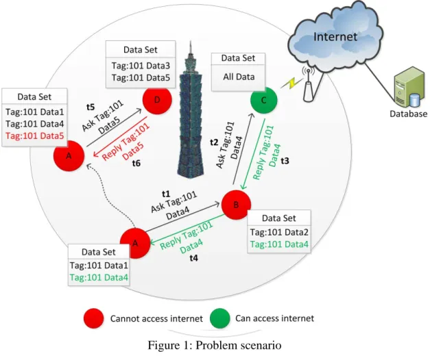
(12) can not connect to the Internet, or even (4) the user never use the mobile network, etc. Both of these scenarios are parts of the disconnect reasons. Despite the user can’t connect to the Internet. If user still wants to send message to someone or search some local information, there is a technique which could achieve user’s requirement, Delay Tolerant Networks. Delay Tolerant Networks is an intermittently connective network [1], all nodes are lacking of continue connectivity [2]. This is used in some place, just like Battlefield [7], Outer space [8], disaster or emergency environment [9] [10], etc. Node-to-Node transfer message is that main feature. However, node sends message to. 治政 the destination by encounter nodes, it will spend much 大time on delivery. But, if you 立 want to send the message out, in DTNs, it is possible to deliver message in spite of the ‧ 國. 學. high transmission time. And we will discuss the related research in Section 2.. ‧ er. io. sit. y. Nat. 1.2 Motivation. al. As we in an area, we want to search some information about that area, but, we. n. iv n C cannot connect to Internet. So what In DTNs, there are two ways to do. h can e nweg do? chi U First, ask the encounter node for the information. If it doesn’t have, we can ask it for help to spread the searching message. This action could increase the searching success probability. We can see Figure 1. At the time t1, Node A wants to search information in this area, but it can’t connect to the Internet. Thus, Node A asks its encounter node B for information. But Node B doesn’t have the information which Node A required. Then Node B helps Node A for searching information. At the time t2, Node B encounters Node C, and Node C can connect to the Internet. So Node B asks Node C for the information, Node C can search in the remote server, and then at time t3, Node C 2 .

(13) replies the information which Node B required. Finally, at the time t4, Node A receives the searching information from Node B. This is a simple scenario we discuss above. In the reality network, it isn’t easy to search information. We have to overcome some issues, and we will discuss it in the next section.. 立. 政治大. ‧. ‧ 國. 學. n. er. io. sit. y. Nat. al. Ch. engchi. i Un. v. Figure 1: Problem scenario. 1.3 Objective Our objective is user in an area could get the information in a shortest time. In order to achieve this purpose, we assume all nodes in the network are collaborative and some nodes can connect to the Internet. The collaborative means all nodes are willing to store other messages into their storage and help other nodes to delivery 3 .

(14) messages. And we don’t consider the incentive issue. Thus, there are some challenge issues we have to discuss, and we divided three parts of these, then described below: 1.3.1 Replication issues (1) Data Replication: Something unique data usually stored in a place or in a node, if we want to get this data, it is difficult to query it. Due to we don’t know where it is, we have to node-to-node ask for the data. It would spend much time to search data, and it would have high probability of searching failure. So, if the data could spread around the network, it would increase the searching. 治政 success probability. But, if the data is unrestricted大 spread, it will cause the higher 立 overhead, like Epidemic. So we have to investigate how to replicate the data, and ‧ 國. 學. how to decide the data transfer. We will describe in Section 3.1.. ‧. (2) Query Replication: Like the Data Replication issue. We want to search. sit. y. Nat. some data, and we have to send query message to get the data. If we have just. io. er. one query copy, it is difficult to get. So, if we can ask the other node for help, it. al. can increase the query success probability. But, we cannot unlimited spread the. n. iv n C query messages and we have to U rule to replicate it. We will h investigate e n g c ha isuitable describe in Section 3.2. 1.3.2 Data Reply issue When the query message looked up the data we want, the replier has to reply the data back to the querier. But, in the network, every node will move, we can’t return the data from the original path. So we have to find the other way to transfer the data. Therefore, we will investigate how the replier response the data to the querier, and this is the most important issue in the thesis. Then, the detail rule we will describe in Section 3.3. 4 .

(15) 1.3.3 Data Synchronize issue This is an independent issue in the thesis. Every node can create new data. If node can’t connect to the remote database server, it just can share the data by the encounter node. If we would like to share this data with every node, we have to sync this data to the remote server. Thus, every node which can connect to the Internet in the network can query this data. Therefore, if we can’t connect to the Internet, we have to ask the node who can connect to for help to sync the data. The detail will be described in Section 3.4.. 立. 政治大. ‧ 國. 學. 1.4 Organization. ‧. The rest of this thesis is organized as follows. Chapter 2 introduces related works. sit. y. Nat. in common DTN routing protocol and the Query-based DTN routing protocol. In. io. er. Chapter 3, we present our searching rule, location-based content search approach. In. al. n. Chapter 4, we present the simulation results. The final, Chapter 5, we concludes this. ni work and discuss the future workCofhthis thesis. U engchi. 5 . v.

(16) CHAPTER 2 Related Work. 政治大 schemes. And we divided the routing protocol into two parts, Common DTN routing 立 In such a variety of DTN routing researches, we focus on query-based routing. ‧ 國. 學. protocol and Query-based DTN routing protocol, the former, we will introduce some common routing approaches, like Epidemic, Spray and Wait etc., and the latter, we. ‧. will discuss the approaches which are related to our work. Then, the routing protocol. Nat. n. al. er. io. sit. y. will be discussed below.. 2.1 Common DTN routingCprotocol h. engchi. i Un. v. We can divide into two kinds of routing protocol: Flooding-based routing and Forwarding-based routing. 2.1.1 Flooding-based routing schemes Flooding-based means node will have a number of the message copies [15], and it will send this copies to all the encounter nodes. We introduce some approaches below. (1) The basic approach, Epidemic [3], whatever nodes encountered, it will send all the messages it have to encounter nodes. It doesn’t have any selection rule, 6 .

(17) just sending until the connection dropped. This approach could get high performance about message delivery success ratio and delivery latency, because a message will be replicated to many nodes, it has high opportunity to send to the destination. But, it will make high overhead, because there are too many redundant messages, and if nodes don’t have enough buffer size, it will overflow quickly. In order to overcome this defect, (2) Spyropoulos et al. proposed Spray and Wait approach [4], they limit the messages replication to L copies, and there are two phase: Spray phase and Wait phase. In Spray phase, when source node encounters another Node B, it will give half copies to Node B to spread these copies.. And the other nodes do the same rule, until. 治政 nodes just have one copy, then they turn to wait phase. 大In wait phase, all the nodes 立 which have the message copy couldn’t send the copy to another node only if they ‧ 國. 學. encounter the destination node. This approach will greatly reduce the transmission. ‧. overhead, but, it just uses the limitation copies, so the message delivery ratio will be. sit. y. Nat. not good as Epidemic. In order to improve this defect, (3) the same authors propose. io. er. an enhance scheme [5]. They change the wait phase [4] where are routed using direct. al. transmission, they let the waiting nodes have the opportunity to send the message out.. n. iv n C It records every encounter timers, h and the timer related e n g c h i U a utility value, then use this value to decide whether delivery or not. This rule will keep the low overhead, and enhance the message delivery ratio. There are some approaches [6][12][16] use the history information to predict the delivery probability and decide the transmission. (4) PRoPHET is the representative of this kind of routing approach. Every node has to maintain a delivery predictability table, and every encounter they calculate new prediction value. When nodes encountered, they compare their prediction value, then. delivery messages to node have highest prediction value. It gets higher delivery rate than Epidemic, but, because of it spends more time to calculate the prediction value and maintain the predictability table, its delivery latency doesn’t well enough. 7 .

(18) 2.1.2 Forwarding-based routing schemes Forwarding-based routing protocols in the network, a message just have one copy [15], and then use different approaches to forward the copy to destination. We introduce some kinds of these schemes, (1) Location-based Routing [17]: it uses GPS to locate nodes position, through different distance algorithm to predict the probability of the message forward to the destination. When nodes encountered, they will compare which one has the highest probability to get to the destination position, then carry it to forward. (2) Gradient Routing: this approach give every node a weighted. 治政 value, and it represents whether this node suitable for大 sending message to receiver or 立 not. Different approaches have different way to calculate weighted value. ZebraNet ‧ 國. 學. [19] uses history of nodes tracking to get the weighted value, then determine message. n. a. 2.2 Query-based DTN routing protocol l. Ch. engchi. er. io. sit. y. Nat. bubbles, and use the ranking value to decide the messages to.. ‧. deliver. In [18], they use social network concept to classify their network node like. i Un. v. In the past research, many papers [3-6, 15-20] focus on how to send data from source node to destination node, and it doesn’t matter the message response problem. It is the one way transmission protocol. If a node sends a request to destination node, it wouldn’t know the message being delivered or not. Therefore, one way transmission is not enough, we have to consider how to response the message that we can look up some information. Several works focus on query in DTNs [11-14, 22], in these papers, not only nodes send request to the message owner, but the owners have to send the response message back. The challenge is all nodes are moving and we don’t know where they going, so asker is difficult to get the answer. We introduce four 8 .

(19) works about this kind of request and response pattern research. Then, it describes below: 2.2.1 Locus: A Location-based Data Overlay for Disruption-tolerant. Networks [11] This research proposed a query mechanism, and use three-tier location area concept (see in Figure 2.a). Let users could look up the relevant information according to its position. Every data object will be given a utility value, and this value. 治政 will vary with the distance between the creation position 大 of data object and the 立 position of the node which carry this data. Figure 2.b shows the changing of the utility ‧ 國. 學. value. If data object near its creation location, the utility of that data object will be. ‧. high. When nodes encountered, they will change their data objects. Before changing. sit. y. Nat. objects, node sorts their data objects by utility value. And the data objects with the. io. er. higher utility value will be sent first. It is because these data objects were created near. al. here. And this rule would let the data objects be centered on its home area, then, users. n. iv n C could query data quickly. But it justhuse the distance between e n g c h i U node and home area, if a node will go out this area, but it is near the home area, encounter node still send data objects to it, then, the transmission is waste. And Locus doesn’t propose an information reply approach, it just uses the multi-copy routing [4][15] to reply data objects.. 9 .

(20) a. Dataa object utiliity region. b. Utility U Funcction. Figure 2: Locus apprroach [11]. 政治大 2.2.2 Perfformance Evaluations E 立 s of Data-ceentric Inforrmation Reetrieval. ‧ 國. 學. Sch hemes for DTNs D [12]. ‧. This reseaarch propossed a compplete approach of dataa search steeps, it inclu udes. y. Nat. io. sit. Data copy, Queery copy and Data replyy. The main n contributee of the reseearch is they y use. n. al. er. Frieendliness Metric M (FM, it is the avverage num mber of nodes it encouunters during an. Ch. i Un. v. obseervation wiindow) to decide d the ddata delivery y. In Data copy, c they ppropose K-ccopy. engchi. repllicate schem me, like thee spray phrrase of Sprray and Waait routing. When Nod de A encoountered Node B, Nod de A will coompare the FM value with Node B, If Nodee B’s valuue greater thhan Node A’s, A it indicat ates Node B will encoun nter more nnodes, and Node N A giives a data copy of the K copies too Node B. Then, T Node A follows tthis rule to send copies until it has h only on ne copy. Thiis is the datta spreading g rule. In Q Query copy, they proppose two schemes, s WSS W (W-coppy selectiv ve query sp praying) annd LNS (L-hop neigghborhood query spray ying). In W WSS, every query havee w numbeer copies, when w noddes encounttered, they compare thhe FM valu ue first, wh hich one haave the hig ghest valuue, the otherr node gavee half query copies to itt, and then keep k spreadding until w = 1. 10 .

(21) In L LNS, it is single-copy y scheme, tthey use L hops to liimit to queery spread. The scheeme doesn’t compare the t FM valuue. When Node N A enccountered N Node B, Nod de A askss Node B foor query data first, if nnot, Node A sends the only o one quuery to Nod de B, thenn the L hopss decreased once. Untill L hops is 0, 0 it doesn’tt spread anyymore. In Reply R Data, this apprroach [12] just j use thee PRoPHET T [6] routin ng scheme tto reply datta to Queerier.. Thiss research assumes the node moving in a fixd d moving paattern, so nodes. could get the accurate a FM M value. Iff nodes move in an un npredictablee path, the FM valuue might be inaccurate... 立. 政治大. 2.2.3 Cooperative Fiile Sharingg in Hybrid d Deelay Tolerant Netw works [13]. ‧ 國. 學. This papeer introducees a Hybridd DTN routiing schemee in file shaaring. In DT TNs,. ‧. som me nodes caan use Wi-F Fi, 3G, etc. connects to t the Intern net, and som me nodes can’t c. sit. y. Nat. acceess Internett. Every data will be diivided into many fragm ments. And every fragm ment. io. er. has a metadata to descript. Then thesee metadata will be spreead out the network. When W. al. q a dataa, it has to find all the metadata of o the data tto download all userr wants to query. n. iv n C the fragments. Like BitTo orrent [23] o fragmennt misses, node n rulee. But, if one h eshares ngchi U couldn’t returnn to the origiinal data.. Figure F 3: Hyybrid DTN example e [13 3] 11 .

(22) 2.2.4 Searching for Content in Mobile DTNs [14] This research focuses on query how to forward and how many queries are replicated. They propose an estimation rule to avoid the query replicates too much. When Node A encountered Node B, Node A will estimate the query had been replicated numbers first. The estimate value is calculated by query hop count and ), if it greater than a. network nodes, then, Node A could get a Utility value (. threshold T, Node A could send the query to Node B. If not, Node A couldn’t. Therefore, if this approach can estimate the query replication number accurately, it. 治政 will greatly decrease transmission overhead and look up 大data efficiently. But, they just 立 use common multi-copy routing schemes to reply data. And the simulation result, they ‧ 國. 學. don’t have compare with other approaches, so we can’t know how this research. ‧. performed.. n. er. io. sit. y. Nat. al. Ch. engchi. 12 . i Un. v.

(23) CHAPTER 3 Location-Based Content Search Approach. 政治大 solve the query problem in case of disruptive Internet connection. In our research 立. We proposed Location-Based Content Search Approach (LCS) in hybrid DTN to. ‧ 國. 學. scenario, all nodes in the network are divided into two types, (1) Online-node and (2) Offline-node. Online-node can connect to the internet to access the remote server, and. ‧. Offline-node cannot connect to that. All nodes have own database and it includes four. sit. y. Nat. tables (see Figure 4), (a) Data Message Table、(b) Encounter Nodes Table、(c) Query. n. al. er. io. Message Table and (d) Reply Message Table. Then we describe below:. i Un. v. (a) Data_table: This table is in charge of the data message storing which is. Ch. engchi. created from node self or received from the other nodes. DataId is the data message unique id, UID is the node id who created this data message, Time is the message creation time or replication time, Data is this message’s content, Sync is whether this message synchronized to the remote server or not. The detail will be described in Section 3.1. (b) ENs_table: This table is responsible for recording encounter node. UID is the node id of the encounter node, Time is the encounter time, Longitude and Latitude is the encounter location. (c) Query_table: This table is in charge of the query message storing, if node is 13 .

(24) Onlline-node, all a query messages aree received from f other Offline-nodde. QryId iss the querry messagee unique id d, Time is tthis messag ge creation time or reeplication time, t QryyMsg is thee content, issQueried is whether th his messagee queried ddata or not. The detaail will be described d in Section 3.22. (d) Replyy_table: thiss table is inn charge off the reply message sttoring whicch is creaated from thhe node thaat received qquery message and had d match dat ata. RepId iss the uniqque id of thiis message, Time is thiis message creation c tim me or replicaation time, Data D is thhe reply datta content, DesUID D is the unique id of the destination nnode. The detail d willl be describeed in Sectio on 3.3.. Data_tablee. 立. 政治大 ENs_table. ‧. ‧ 國. 學. n. er. io. sit. y. Nat. al. Q Query_table e. Ch. engchi. iv n R e U Reply_table. Figure 4: Databasee Tables. In this theesis, our go oal is wish the Offlinee-node could d get the innformation they needd by the other nodes as soon ass possible. In order to o reach thiss objective, we 14 .

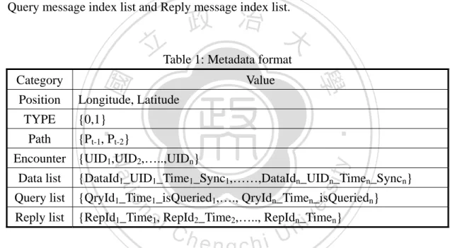
(25) propposed four strategies to solve thhis problem m, (1) Dataa replicationn strategic,, (2) Queery replicattion strategiic, (3) Dataa reply straategic, (4) Data synchhronization and upddate. In this theesis, we asssume the arrea range is known, and we divideed the area into threee parts, Inside Area, Border Area and Outsidee Area, and it shown ass Figure 5.. 政治大. 立. ‧. ‧ 國. 學 er. io. sit. y. Nat. al. n. Three parts area figure Figure 5: T. Ch. engchi. i Un. v. n a radius oof γ meterss from area central, ouutside the In nside Inside Areea is within Areea. meterss is Border Area A and thhe other areaa is Outsidee Area. Thiss intention is i let. noddes in differeent area usee different w ways to seleect messagees and delivver messagees. In ordeer to identiffy the node position, w we refer to th he Vincenty y’s formula[[26](Formu ula 1, detaail see the [26]), [ this formula fo connsidered thee earth is elllipsoid, andd use Longiitude and Latitude tw wo points to o calculate the shortest distance s, and the ddeviation caan be accuurate to 0.5 millimeter. We use thhe node posiition point and a the Areea Central Point P (CP P) to calculaate the distan nce d, if. ≤ , it indiicates the no ode is in thee Inside Areea, if 15 . .

(26) > . ≤. +. , it indicates the node is in the Border Area, if >. +. , it. means the node is in the Outside Area.. =. ( −∆ ). (1)[26]. When two nodes encounter, they will change their metadata first (shown as Table 1), it includes node’s position, node’s type (Online-node or Offline node), node past moved path point, node encounter nodes, node collected Data message index list, Query message index list and Reply message index list.. 政治大. Position Path. Value. Longitude, Latitude {0,1}. ‧. TYPE. 學. Category. ‧ 國. 立Table 1: Metadata format. {Pt-1, Pt-2}. y. sit. Data list. Nat. Encounter {UID1,UID2,…..,UIDn}. {DataId1_UID1_Time1_Sync1,……,DataIdn_UIDn_Timen_Syncn}. io. {QryId1_Time1_isQueried1,…., QryIdn_Timen_isQueriedn}. Reply list. {RepId1_Time1, RepId2_Time2,….., RepIdn_Timen}. n. al. er. Query list. Ch. engchi. i Un. v. When two nodes encountered, we call ourself as Node A, encounter node as Node B, the Location-based Content Search approach (LCS) workflow is shown as Figure 6, and the transmission protocol is shown as Figure 7. First, Node A and Node B always detect connection, when encountering, Node A will send a metadata request to Node B, after receiving the request, Node B returned its metadata to Node A, when Node A received the metadata from Node B, the first step is check and filer the identical messages from Node A’s database, then keep the message which Node B doesn’t have, and rebuilt that metadata. The next step is Message Selection, it selects the messages which can be sent to Node B. There are three strategies step we 16 .

(27) proposed to select the messages, (1) Data replication strategic, Node A selected the Data messages according to Node A’s position. The detail description is in Section 3.1. (2) Data Reply strategic, get the Query message from metadata, if Node A’s database have the queried data message, Node A will generate a Reply message. The detail description is in Section 3.2. (3) Query replication strategic, this strategic must be handled after Data Reply strategic complete, and the queries which queried data shouldn’t send out anymore. The detail description is in Section 3.3. After completing three message selection steps, Node A has chosen the messages which will be sent to Node B. The next step, Node A will check the Data messages which doesn’t. 治政 synchronize to the remote server. If Node A is an Online-node, 大 it will sync this Data 立 messages to the server, if not, Node A doesn’t do anything, and the detail will be ‧ 國. 學. described in Section 3.4. Before sending messages to Node B, Node A has to schedule. ‧. to messages which will be sent first. Because of the contact time of two nodes are. sit. y. Nat. short, it couldn’t send all the messages to the other nodes. Therefore, how send the. io. er. messages to the encounter node efficiency, it is shown in Section 3.5. Then, Node A. al. sends the selection message queue to Node B. As Node B receiving, it will check the. n. iv n C Data messages whether it sync to h server or not. If Node e n g c h i U B is an Online-node, then sync the message to server, if not, skip this action, and then finish this contact.. 17 .

(28) 立. 政治大. ‧. ‧ 國. 學. n. er. io. sit. y. Nat. al. Ch. engchi. i Un. v. . Figure 6: LCS workflow. 18 .

(29) 立. 政治大. ‧. ‧ 國. 學. n. er. io. sit. y. Nat. al. Ch. engchi. i Un. v. Figure 7: LCS transmission protocol 19 .

(30) 3.1 Data replication strategic When two nodes encountered in the map, the processing step can be seen in Figure 8, and the selection rule is shown in Formula 2, (1) If the distance d between Node A and Area Central Point (CP) is less than or equal to radius γ, it indicates Node A is in the Inside Area. When Node A encountered Node B, it will add all the Data messages into the Data dataset D_set to prepare to send to the Node B. The main purpose is let the Inside Area fulfill with related Data messages. If any node wondered to query in this area, it can get the Data messages quickly and has high query success. 治政 rate. But the encounter time of the two nodes and the 大transmission are limited, two 立 nodes have to change itself metadata before transport. Then, Node A skips the ‧ 國. 學. identical Data messages, and adds the others into D_set; (2) If the distance d between. ‧. Node A and CP is greater than radius γ and less than γ + , it indicates Node A is in. sit. Nat. < 0, it indicates Node B. y. .. the Border Area. According to Node B’s past path, if ∆. er. io. will likely enter to the Inside Area, then, Node A add the Data messages into the. n. D_set; (3) if the distance d a between Node A and CP is greater i v than γ + , it indicates l. Ch. n engchi U. Node A is in the Outside Area, then, Node A shouldn’t do anything. We use ∆ In Formula 3, t-1, and. .. to predict whether Node B’s will enter to the Inside Area or not.. .. is the distance between Node B position Pt-1 and CP at time. .. Then, subtract. is the distance between Node B position Pt-2 and CP at time t-2. .. from. .. , if the result is less than 0, it means Node B is. likely to enter to the Inside Area, if the result is granter then 0, it means Node B is likely to move away from the Inside Area.. 20 .

(31) (. , _. )=. ,. .. ≤. ,. .. >. ,. ∆. .. .. ≤. +. ℎ. =(. .. −. .. ∆. 2. .. < 0. (2). . ). (3). In order to avoid data overflow, we set all the Data messages a storing time TTS (Time-to-Store) (Formula 4). TTS means the time of any message be created or replicated then store in some node. When TTS expired, the messages will drop anymore. Therefore, it can reduce the node loading.. 立. _ _ ,. ℎ. (4). ‧. ‧ 國. . ,. )=. 學. (. 政治大. Otherwise, if Node B is an Online-node, Node A doesn’t need to send Data. Nat. sit. y. messages to Node B. Because the Online-node can connect to the Internet to get the. n. al. Ch. . engchi. 21 . er. io. messages by itself, it doesn’t require wasting the resource to send messages.. i Un. v.

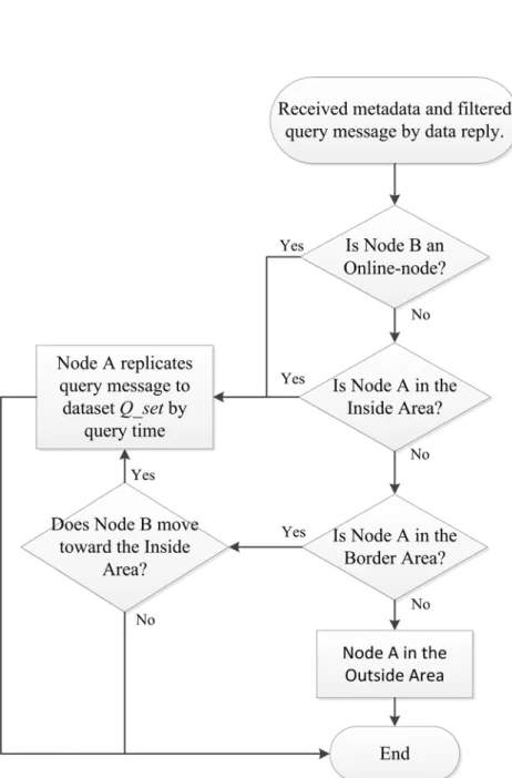
(32) 立. 政治大. ‧. ‧ 國. 學 er. io. sit. y. Nat. al. . v. n. Figure 8: Data replication strategic flow chart . Ch. engchi. i Un. 3.2 Query replication strategic This strategic has to do after the Data reply strategic, and the goal of this strategic is let user queried data in a shortest time. This is a three-tier Query strategic, from Node A’s local database to Node B’s local database then remote server. Query replication detail rule can see in Formula 5 and Figure 9 flow chart. When Node A receiving query messages, it has to check the database whether the query messages have the match data. If has, it doesn’t need to do Query replication, if not, there are some rules to do. (1) Node A is an Online-node. It does nothing. (2) Node A is an 22 .

(33) Offline-node. When Node A in the Inside Area, and then adds all the related Query messages to the Query dataset Q_set; When Node A in the Border Area, then Node A has to predict Node B’s direction ( ∆ is shown in Formula 3), if ∆. .. . , the detail can see in Section 3.1, and also. less than 0, it indicates Node B is likely to enter to. the Inside Area, then, add the related Query messages to the Q_set. If not, then do nothing. The main purpose is Data replication strategic will centralize the related Data messages in the Inside Area. Therefore, we send the queries to the Inside Area, and there is more opportunity to query success. It has two reasons. One, There are many related messages in the Inside Area. The other, if any node leave from Inside Area, we. 治政 expect it could carry much more related messages; When 大Node A in the Outside Area, 立 it shouldn’t do anything. ‧ 國. 學. In addition, if the query represents it had been queried (. y ,. . > . ℎ. (. , , ,. al. ≤. . )= =. ≤. Ch . engchi U. +. sit. .. . ∆ . < 0 2 . er. )=. n. , _. ,. io. Nat. (. =. ‧. ), then we don’t have to add this query into the Q_set.. .. v ni. (5). However, if we don’t have any limitation of replicate query message, it will keep replicating in spite of it has queried. Therefore, we need a mechanism to stop it. Every Query messages set a TTS, if the TTS expired (Formula 6), and then drop it. This way will inhibit query replication. There are some defects in the way. If TTS is too short, it would query data hardly. If TTS is too long, it would still create many query copies. So we add one more rule. If query message find the match data, this query message’s attribute isQueried will be change to TRUE. And next time, nodes encountered, they 23 .

(34) change their metadata, then nodes will know what query message had been queried, and it will skip it to add to Q_set.. ( . ,. )=. _ _ ,. (6). ℎ. . . 立. 政治大. ‧. ‧ 國. 學. n. er. io. sit. y. Nat. al. Ch. engchi. i Un. v. Figure 9: Query replication strategic flow chart. 24 .

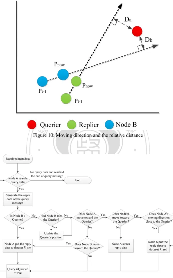
(35) 3.3 Data Reply strategic As shown in Figure 11. Node A received Node B’s metadata, it will check all query messages of Node B’s metadata. If Node A has the match data, it will generate a Reply data R_data of the Query message and change the Query message attribute. isQueried to TRUE, then we can call Node A as Replier. It is difficult to send the Reply data to the Querier. Because all nodes in the network are keeping moving, we can’t use the original packet delivery path to send back to the Querier. Therefore, we have to use the other rule to send Reply data.. 治政 Replier (Node A) can know the Querier’s location 大 from Query message, and 立 send the Reply data to that location. But, as time goes by, Querier may not still stay ‧ 國. 學. there. So, when Replier (Node A) encounters other node (Node B), it will check the. ‧. Encounter Table of Node B whether it had encountered Querier or not. If it had, we. sit. y. Nat. will check the encounter time whose close the recent time. If Node B’s encounter time. io. (. . , ,. =. al. n. metadata.. er. close, we will update (Formula 7) the Querier position of Replier’s (Node A). ( ℎ. Ch. ) ∈ . _. engchi ). (. .. i Un. v. >. .. ) . (7). Then we have to distinguish which Node will move toward to the Querier, see the Formula 8, if Replier (Node A) won’t move toward to the Querier but Node B will do, it would add the R_data to the Reply dataset R_set. Otherwise, Replier (Node A) will move toward to the Querier but Node B won’t, it just keeps the R_data and does nothing. 25 .

(36) ( _. =. ). , _ , , , , ,. ( (. . .. )= )=. . .. (. )= )= ) ) . . . ( & ( > &( >. (8). If Replier (Node A) and Node B are moving the same direction and forward to the Querier, we have to calculate whose moving path will close to the Querier. In Figure 10, we can use the position Pnow , the past position Pt-1 to determine this node’s moving direction, then we add the Querier position Pq and use the basic Triangle Area. 政治 , as大 we know the distance between. formula (Formula 9) to calculate the area value. 立. Pnow and Pt-1, we can get the close Querier distance D. If Da greater than Db, it. ‧ 國. 學. indicates Node B will move close to the Querier, then we add the R_data to the R_set and waiting for transmission. Otherwise, If Da less than Db, it indicates Replier (Node. ‧. A) will move close to it, then we just keep the R_data and moving.. n. 1 2. er. io. al. sit. y. Nat =. Ch. engchi. i Un. (9). v. However, we could not replicate messages unlimited, so we have to make some rule to inhibit it. All the Reply data will set a TTS, when the TTS expired or R_data had forwarded to the querier , this message R_data will drop anymore (Formula 10).. ( _. )=. , , ,. _. _ _ ℎ. ℎ. ℎ. 26 . . (10).

(37) 立. 政治大. ‧ 國. 學. . Figure 10: Moving direction and the relative distance. ‧. n. er. io. sit. y. Nat. al. Ch. engchi. i Un. v. . Figure 11: Data reply strategic flow chart 27 .

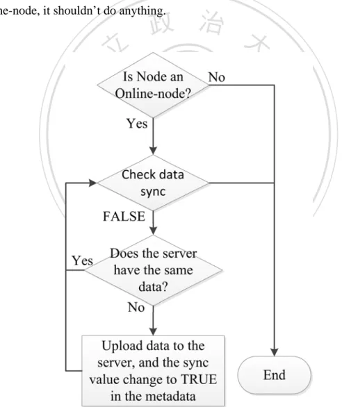
(38) 3.4 Data synchronization and update strategic Whatever Online-node or Offline-node, it would create data messages. Beside keeping the data in local database, it has to upload this data messages to the remote server to share this information. Figure 12 shows this strategic. When node received messages, the first step is distinguishing the type of node, if it is Online-node, it should upload all the data messages which doesn’t sync to the remote server directly. Then change the Sync attribute of this data message to TRUE. Otherwise, if it is Offline-node, it shouldn’t do anything.. 立. 政治大. ‧. ‧ 國. 學. n. er. io. sit. y. Nat. al. Ch. engchi. i Un. v. Figure 12: Data sync and update strategic flow chart. 28 .

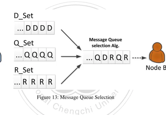
(39) 3.5 Message queue selection algorithm When all the messages are chosen (D_set, Q_set and R_set), Node A has to send these messages to Node B. But the messages cannot be parallel transferred. Therefore, we have to decide which one will be sent first. In the thesis, shown in Figure 13, we proposed a simple message queue selection algorithm, within the weight value d, q and r, and progressive value S to calculate and get the transmission Message queue M.. 立. 政治大. ‧. ‧ 國. 學 er. io. sit. y. Nat. al. v. n. Figure 13: Message Queue Selection. Ch. engchi. i Un. We can get the dataset D_Set, Q_Set and R_Set from all the replication strategies we describe above. Then we give the dataset a different weight value d, q, r and d + q + r = 1. The first step, we find the dataset of highest weight value MaxSet, then, the MaxSet dataset pop a message and enqueue to M. This will be the first transmission message, then, we reset the weight value of MaxSet dataset, and add the Progressive value S to the other weight. Repeat the steps until all messages enqueue to M, and then we can get a complete Message queue M. Finally, Node A according to M sends all the messages to Node B. The beginning results of this selection queue are similar to Weight Fair Queue 29 .

(40) (WFQ), the highest weight of messages will be sent more. After several times, the message will be selected by Round Robin (RR), because of the weight value and progressive value.. Message queue selection algorithm Input: Data dataset D_set, Query dataset Q_set, Reply dataset R_set, Data weight d, Query weight q, Reply weight r, Progressive value S Output: Message queue M While((size(D_set) + size(Q_set) + size(R_set)) != 0) MaxSet = Max(d,q,r).getSet() M.enqueue(popMsg(MaxSet)) Switch(MaxSet) Case D_set: d = d.original, q = q + S, r = r + S Case Q_set: d = d + S, q = q.original, r = r + S Case R_set: d = d + S, q = q + S, r = r.original End switch If size(MaxSet) = 0 then MaxSet.weight = 0 End while Return M. 立. 政治大. y. sit. n. er. io. al. Ch. engchi. 30 . ‧. ‧ 國. 學. Nat. 1: 2: 3: 4: 5: 6: 7: 8: 9: 10: 11:. i Un. v.

(41) CHAPTER 4 Simulation Results. In this chapter, we discuss the simulation results, and we compare with three. 政治大. protocols. LCS (we proposed), Locus [11] and Epidemic [3]. We make some variation. 立. in Epidemic, because of Epidemic doesn’t matter the query-reply situation. We set the. ‧ 國. 學. area concept and let nodes having query scenario and reply action in Epidemic. Then, in the results, we will show some validation parameters. And we explain. ‧. how the equation be calculated below.. y. Nat. io. sit. (1) Query-Reply Success Ratio: The equation is shown below. The number of. n. al. er. success reply message means all the reply messages success delivery from Replier to. Ch. i Un. v. Querier, and the same data we won’t be repeatable recorded. And the number of query. engchi. message means how many numbers the query message be generated, so the replicate query messages we won’t record. (2) Query Delivery Ratio: The equation is shown below. The number of query delivered means the all query messages which delivered to the data source node and the number of query message described above. (3) Overhead: The messages which are redundant transferred are overhead. Success reply message means the first message reply to the Querier and the same messages replied afterword do not include. Query delivered means the first message delivered to the Replier, and as above, the same messages don’t include. 31 .

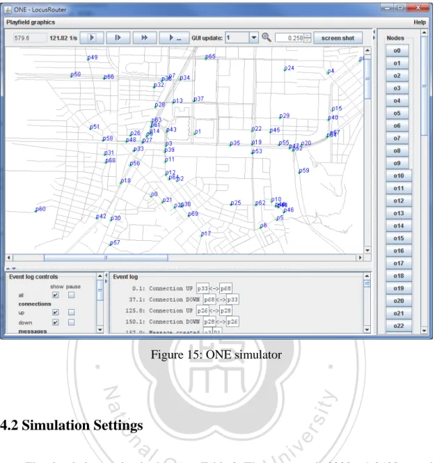
(42) (4) Latenccy: We calcculate from the time of send the first f query m message by y the Queerier to the time of recceive the firrst reply meessage by th he Replier. And the results we gget the meddium numbeer to analyzee.. z. Query-Reeply Successs Ratio =. z. Query Delivery Ratio o=. z. Overhead =. z. Latency = Time (Recceived first rreply messagge) − Time (sent first qquery messaage). #. #. #. 4.1 Simulatiion Setup. 立. #. #. 政治大. ‧ 國. 學. We use ONE(Oppor O rtunistic N etwork Env vironment simulator) [27](shown n as. ‧. Figuure 15) andd the map of Taipei1001 surround ding area (F Figure 14) to validatee our. sit. y. Nat. apprroach. All nodes are pedestrian, p and we sett a random destinationn point to th hem.. io. al. n. n by shortesst path algorrithm. noddes move to the position. Ch. engchi. er. When they reaached the deestination, tthen we giv ve them the other destiination. And all. i Un. v. Figuree 14: Map oof Taipei101 1 surroundin ng area 32 .

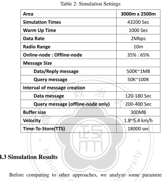
(43) 立. 政治大. Nat. sit. y. ‧. ‧ 國. 學 Figure 15: ONE simulator. er. io. 4.2 Simulation Settings. al. n. iv n C The simulation setting is shown 2. The map area is 3000m * 2500m, and h ase Table ngchi U the simulation time is 43200 seconds, it is equivalent to 12 hours. In order to initialize data sources, we have to set a warm up time 1000 seconds. The node data transmission rate is 2Mbps, and the transmission rage is 10m. All nodes divided to types, 35% is Online-node and 65% is Offline-node. The message size of Data message and Reply message are 500KB~1MB, and the Query message is 50KB~100KB. All the messages have a creation interval, the Data message is 120~180 seconds, and the Query message is 200~400 seconds. The node buffer size is 500MB. All nodes are pedestrian, so the moving speed is 1.8km~5.4km per hour. And the messages’ TTS is 18000 seconds, it is equivalent to 5 hours. 33 .

(44) Table 2: Simulation Settings Area . 3000m x 2500m . Simulation Times . 43200 Sec . Warm Up Time . 1000 Sec . Data Rate . 2Mbps . Radio Range . 10m . Online‐node : Offline‐node . 35% : 65% . Message Size . . Data/Reply message . 500K~1MB . Query message . 50K~100K . Interval of message creation . 治政 Data message 120‐180 Sec 大 Query message (offline‐node only) 200‐400 Sec 立 Buffer size . 300MB . ‧ 國. 學. Velocity . 1.8~5.4 km/h . Time‐To‐Store(TTS) . 18000 sec . ‧ y. Nat. n. er. io. al. sit. 4.3 Simulation Results. i Un. v. Before comparing to other approaches, we analyze some parameters to our. Ch. engchi. approach. First we will discuss the effect of the percentage of node type and the radius of Inside Area. Then, we will compare with other approaches to analyze the performance. And we will discuss below. 4.3.1 The percentage of node type We simulate four node type scenarios. All the Online-node can’t query data, because we assume they can query from the Internet directly. They just create or reply data. We can see Figure 16 Query-Reply success ratio. If there are no Online-nodes, it get low success ratio. Because all nodes are Offline-node, they can’t know all the data 34 .

(45) messsages.. 立. 政治大. ‧ 國. 學. Figure 16 6: Query-Reeply Successs Ratio (No ode Type). ‧. n. er. io. sit. y. Nat. al. Ch. engchi. i Un. v. Figuree 17: Queryy Delivery Ratio R (Nodee Type). Thus, theyy cannot geet data easilyy. They hav ve to spend more time (see Figuree 19) and more repliicate (see Figure F 18) to find thee data. And d we can seee Figure 17 to valiidate our oppinion, in th he first casee (0% vs. 100%), it geet the worstt query deliivery 35 .

(46) ratioo. Howeverr, if the netw work full off Online-nod de, it meanss they don’tt need any more m repllication (low w overhead)), because itt is easily to o encounter Online-nodde, and they y can direectly ask theem for dataa. So, they gget the data quickly (lo ow latency) . Therefore, the fourrth case (900% vs. 10%)) is the bestt results of all a the chartss.. 立. 政治大. n. er. io. al. Ch. engchi. i Un. Figure 19:: Latency (N Node Type) 36 . sit. y. ‧. ‧ 國. 學. Nat. Figure 18: Overhead (Node Type)). v.

(47) 4.3.2 Rad dius of Insid de Area We show the resultss of radius changing. In Figure 20, it is thhe Query-R Reply succcess ratio, and a we can n see the sm mall radius performed a bad resuult. Becausee our apprroach doesnn’t matter th he outside aarea, if the radius r too sm mall, there aare a few nodes in thhe Inside Area, and theen the relateed data doessn’t be centrralized in thhe area. And d the big radius perrformed bad dly, too. B Because the large Inside Area w will allow more m messsage replication, and the t data willl be more complicated c d and be sprread around d this big area, then, it is more difficult to look up daata. So, the suitable raddius is betw ween 3000 and 500.. 立. 政治大. ‧. ‧ 國. 學. n. er. io. sit. y. Nat. al. Ch. engchi. i Un. v. Figgure 20: Query-Reply S Success Rattio (Radius of Inside Arrea). As w we discuss above, there are a few w nodes in the small radius r of innside area, so, s it doesn’t have much m replicaation activitty, if any no ode would like to queryy in this areea, it willl spend muuch time to search thee data sourcce. Then, in n Figure 2 1, it perforrmed 37 .

(48) low wer overheadd in the smaall radius. O On the otherr hand, in th he big radiuus, it got hiigher overrhead. Andd in Figure 22, 2 nodes sppent much time to queery in the sm mall radius,, and in thhe big radiuus, nodes wo ould look up quickly. Otherwise, O the t selectedd results basse on the environmennt settings. If there aree different transmission t n ranges, buuffer size, node n speeed, etc., we might get the t differennt suitable raadius. The radius r 500m m is the suittable sizee in our scennario.. 立. 政治大. ‧. ‧ 國. 學. n. er. io. sit. y. Nat. al. Ch. i Un. v. us of Inside Area) Figurre 21: Overhhead (Radiu. engchi. Figu ure 22: Latenncy (Radiuss of Inside Area) A 38 .

(49) 4.3.3 Node Density In the section, we analyze the results with other approaches, Locus and Epidemic routing schemes. And we want to see what the importance part of our approach is, so we make two changing in our approach. One is we don’t matter the Data replication strategic and we only use the Epidemic routing to spread the data messages, and the other is we don’t care the Query replication strategic, just use Epidemic to disseminate the query messages. In Figure 23, we can see our approach and Locus have a similar performance in. 治政 query-reply success ratio, because both of we are大 using the region concept to 立 centralize the messages. But, as the number of nodes increase, Locus will perform ‧ 國. 學. well than ours. Because our region concept base on local area, if there are many nodes. ‧. in this area, it will have many messages (data, query, reply) in every node. Although. sit. y. Nat. nodes have rich data source, the transmission rate is fixed, and nodes intermittent. io. er. connected, they can’t send all the messages. So, some messages might be ignore, and. al. the performance isn’t well. And we want to see the importance part of our approach,. n. iv n C we modify it in two types. (1) We use routing to replace the data replication h eepidemic ngchi U strategic, and (2) we use epidemic routing to replace the query replication. The result shows the (1) type got worse performance. Because the data messages couldn’t be centralized to the inside area, the messages would spread to whole network. It is difficult to query unique data message in the network. Otherwise, in order to compare fairly, we present a scenario with only Offline-node in our approach. Although the success ratio is worse than Locus, but the overhead and latency are better than Locus. And the result will discuss below.. 39 .

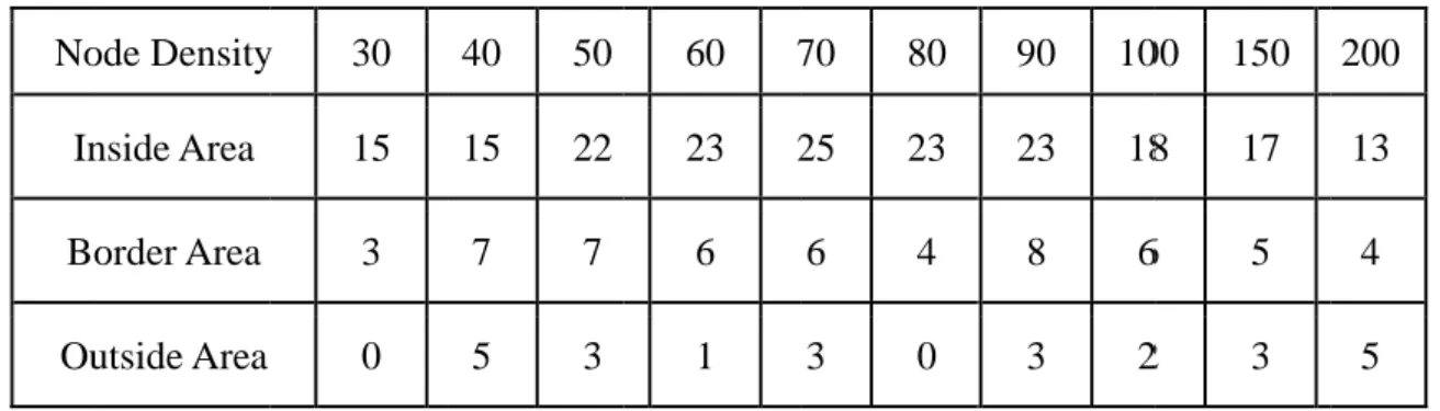
(50) 政治大. Figure 23: Query-Repply Success Ratio (Nod de Density). 立. . ‧ 國. 學. And we caan see the Figure F 24 annd Table 3, in our apprroach, theree are 71% of the noddes success searching data d in Insidde Area. It means nod des in the Innside Area will. ‧. have high probbability to qu uery successs.. n. er. io. sit. y. Nat. al. Ch. engchi. i Un. v. Figure 24: 2 Node Diistribution of o Success Searching S. 40 .

(51) Tablee 3: Detail number n of N Node Distrib bution in Su uccess Searrching Noode Densityy. 30. 40. 50. 60. 70 7. 80. 90. 1000. 150. 200. Innside Area. 15. 15. 22. 23. 25 2. 23. 23. 188. 17. 13. Border Area. 3. 7. 7. 6. 6. 4. 8. 6. 5. 4. Ouutside Area. 0. 5. 3. 1. 3. 0. 3. 2. 3. 5. Figure 25 shows the query q delivery ratio, we w define thee query deliivery as Querier sentt the query message, m an nd it deliverry to the Reeplier who has h the data source. Wee can. 政治大. see the figure,, all the ap pproaches hhave high delivery d rattio, becausee data message. 立. doesn’t just one copy spreead to the neetwork, and d the query message m dooes, either. In I all. ‧ 國. 學. the query messsages, we ju ust need onee query messsage to find d the data soource, then,, it is succcess deliverry. Thereforre, it is easyy to find thee Replier, bu ut how to reeply this daata to. ‧. the Querier is the t most diffficult.. n. er. io. sit. y. Nat. al. Ch. engchi. i Un. v. Figure 25: Query D Delivery Raatio (Node Density) D. Figure 266 is overheaad, and we can see thee result of Locus, L althhough the query q o Locus iss higher thhan LCS, but b its overrhead is larrger than LCS. L succcess ratio of 41 .

(52) Beccause Locuss centralizes the same data in thee same areaa, if Querieer closed to this areaa, it can usee a few querry replicate to look up data quicklly. But, if Q Querier far away a from m this area, it has to reeplicate moore messagee in delivery y. So the ovverhead will be highher. And LC CS is a wid de range of the local arrea, it spreaads all the m messages in n the areaa, thus, LCS S has higherr opportunitty to spend lower l cost to t get the daata.. 立. 政治大. sit. io. er. . y. ‧. ‧ 國. 學. Nat. Figure F 26: O Overhead (N Node Density y). al. Figure 27 is Query Latency. L Wee can see thee result of our o approacch LCS is much m. n. iv n C wer than Loccus and Ep pidemic. Be low U willl be spreadd in the areea, if hecause e n gallcthhheidata nodde in the Inside Area orr Border Areea, it will qu uickly get th he data. Altthough Locus is usedd the area concept, c too o. They wiill centralizee the same data in thee area, if nodes wannt to query that data, but b they arre not near the area, itt will spendd much tim me to querry data.. 42 .

(53) 政治大. Figure F 27: L Latency (No ode Density y). 立. ‧ 國. 學. 4.3.4 Bufffer Size. Figure 288 shows thee query-repply success ratio. We can see thhe result off our. ‧. apprroach LCS S and Locu us. As the buffer sizee increased,, nodes couuld store more m. y. Nat. io. sit. messsages, andd it could increase i thee query succcess probaability. Ourr approach and. n. al. er. Loccus have sim milar rule to t replicate messages, so the success ratio aare similar. But. Ch. LCS S has the addvantage of overhead an and latency.. engchi. i Un. v. Figure 28 8: Query-Reeply Successs Ratio (Bu uffer Size) 43 .

(54) Figure 299 is the oveerhead. As tthe buffer size s increasse, all the ooverhead off the apprroaches inccrease slowly. Becausee node has more spacee to store m messages, when w noddes encounteered, they can c send m more messag ges. But thee transmissiion rate and d the encoounter timee are limited d, it can’t sennd more as buffer size increased.. 立. 政治大. n. sit. er. io. al. y. ‧. ‧ 國. 學. Nat. . Figure 29: O Overhead (B Buffer Size). i Un. v. Figure 300 is the queery latency. As the bu uffer size in ncrease, all the approaaches. Ch. engchi. ve more spaace to storee messages, it is decrrease the laatency resullts. Becausee nodes hav posssible to forrward the reeply messagge to the Replier. R Our approach L LCS is the best one in all the results. We W use the llocal region n concept to determinne the message forw warding, annd the big storage coould store more m imporrtant messaages, like reply r messsage, then, it could enh hance the ddelay time of query-replly activity.. 44 .

(55) 政治大. Figure 30: Latency (B Buffer Size). 立. ‧ 國. 學. 4.3.4 Tim me to Store. ‧. This sectioon we wantt to see the iinfluence of messages live time chhanging. Figure. y. Nat. io. sit. 31 sshows the query-reply q success raatio results, we can seee the low T TTS parameeters,. n. al. er. everry approachh display thee bed perforrmance, beccause messaages just hav ave short tim me to. Ch. i Un. v. livee, they don’t have mucch time to ddelivery, so the successs ratio doessn’t well. In n the. engchi. low w TTS, Locuus is worse than LCS, it is becausse they will try their beest to centraalize the data in its area, but th he live timee of data isn n’t enough, it drops quuickly, so nodes are difficult to query data.. 45 .

(56) 政治大. Figure 31: Queryy-Reply Succcess Ratio (TTS). 立. ‧ 國. 學. Figure 32 shows the overhead reesults, as th he TTS grow wth up, the overhead of o all the approachess will increease. Becauuse messag ges have a long time to stay in n the. ‧. netw work, if repply messagees success ddelivery to the t Querierr, the other message which w. y. Nat. n. al. er. io. incrrease the ovverhead.. sit. doesn’t send to t the Querrier still exxist in the network. Then, T these messages will. Ch. engchi. i Un. Figure 332: Overheaad (TTS) 46 . v.

(57) Figure 33 shows the latency ressults. As th he TTS growth, the lattency of alll the apprroaches willl increase. Because theere are man ny messages in every nnode, and in n the sendding queue,, the old meessage will bbe sent firstt. So the new w one is diffficult to be sent, thenn, it could sppend much time to forw ward.. 立. 政治大. n. sit er. io. al. Ch. engchi. 47 . y. ‧. ‧ 國. 學. Nat. Figure 33: Latency y (TTS). i Un. v.

(58) CHAPTER 5 Conclusions and Future Work. 政治大 four strategies to achieve our objective. It is Data replication strategic, Query 立. In this thesis, we proposed a location-based content search approach. We use. ‧ 國. 學. replication strategic, Data reply strategic and Data synchronize and update. Then we proposed a three-tier area concept, and every strategic in different area will have. ‧. different rule to replicate messages. We divided all nodes into two parts, Online-node. Nat. sit. y. and Offline-node. If Offline-node wants to search some information, besides the other. n. al. er. io. Offline-node, it can ask Online-node for searching. And in the sending message. i Un. v. period, we proposed a message queue selection algorithm to decide which message. Ch. engchi. will be sent first. Finally, we evaluate the results with Epidemic and Locus. And we use some parameters to verify our approach. Although LCS is worse than Locus in Query-Reply success ratio, in Overhead and Latency, LCS is much better than Locus. In the future, we will consider the adaptive weighted value of messages. According to the message forwarding times or the estimation numbers of unique messages in some area. The weighted value of messages could be revised, and the nodes can spread the most important message out. Finally, we will implement this work into Plastory [28] system which is a mobile storytelling platform we developed before. 48 .

(59) REFERENCE. [1] V. Cerf, S. Burleigh, A. Hooke, L. Torgerson, R. Durst, K. Scott, K. Fall and H. Weiss, “Delay-Tolerant Networking Architecture”, RFC4838, April 2007, [Online].. 政治大 [2] K. Fall, “A Delay-Tolerant Network Architecture for Challenged Internets”, In 立 Proc. SIGCOMM, August 2003. Available: http://www.ietf.org/rfc/rfc4838.txt. ‧ 國. 學. [3] A. Vahdat and D. Becker, “Epidemic routing for partially-connected ad hoc networks,” Tech. Rep. CS-2000-06, Duke University, July 2000.. ‧. [4] T. Spyropoulos, K. Psounis, C.S. Raqhavendra, “Spray and wait: an efficient. y. Nat. io. sit. routing scheme for intermittently connected mobile networks”, EE, USC, USA, In. n. al. er. Proc. SIGCOMM, August 2005.. Ch. i Un. v. [5] T. Spyropoulos, K. Psounis, C.S. Raqhavendra, “Spray and Focus: Efficient. engchi. Mobility-Assisted Routing for Heterogeneous and Correlated Mobility”, USC, EECS, USA, In Proc. PERCOM, March 2007. [6] A.Lindgren, A.Doria, and O. Schel’en, “Probabilistic Routing in Intermittently Connected Networks”, LUT, Sweden, In Proc. SIGMOBILE, vol. 7-3, July 2003. [7] D.K. Cho, C.W. Chang, M.H. Tsai, M. Gerla, “Networked medical monitoring in the battlefield”, CS, UCLA, USA, In Proc. MILCOM, November 2008. [8] C. Caini, P. Cornice, R. Firrincieli, D. Lacamera, S. Tamagnini, “A DTN Approach to Satellite Communications”, DEIS/ ARCES, University of Bologna, Italy, In Proc. IEEE Journal on Selected Areas in Communications, vol. 26-5, June 2008. 49 .

(60) [9] Y. Sasaki, Y. Shibata, “Distributed Disaster Information System in DTN Based Mobile Communication Environment”, Japan, In Proc. BWCCA, November 2010. [10] P. Jinag, J. Bigham, E. Bodanese, “Adaptive Service Provisioning for Emergency Communications with DTN”, EECS, Queen Mary University of London, UK, In Proc. WCNC, March 2011. [11] Nathanael Thompson, Riccardo Crepaldi and Robin Kravets, “Locus: A Location-based Data Overlay for Disruption-tolerant Networks”, CS, University of Illinois Urbana-Champaign, USA, In Proc. CHANTS, September 2010. [12] P. Yang, M.C. Chuah, “Performance evaluations of data-centric information. 治政 retrieval schemes for DTNs”, CSE, Lehigh University, 大 USA, In Proc. MILCOM, 立 November 2008. ‧ 國. 學. [13] Cong Liu, Jie Wu, Xin Guan and Li Chen, “Cooperative File Sharing in Hybrid. ‧. Delay Tolerant Networks”, In Proc. ICDCSW, June 2011.. sit. y. Nat. [14] Mikko Pitkänen, Teemu Kärkkäinen, Janico Greifenberg, and Jörg Ott,. io. er. “Searching for Content in Mobile DTNs”, Helsinki University of Technology, Finland,. al. In Proc. PERCOM, March 2009.. n. iv n C [15] S.C. Nelson, M. Bakht, R. Kravets, Routing in DTNs”, CS, h e n “Encounter–Based gchi U University of Illinois at Urbana-Champaign, USA, In Proc. INFOCOM, April 2009. [16] E.C.R de Oliveria, C.V.N. de Albuquerque, “NECTAR: A DTN Routing Protocol Based on Neighborhood Contact History”, Universidade Federal Fluminense, Brasil, In Proc. SAC, March 2009 [17] J. LeBrun, C.N. Chuah, D. Ghosal, M. Zhang, “Knowledge-Based Opportunistic Forwarding in Vehicular Wireless Ad Hoc Networks”, UC Davis, USA, In Proc. VTC, May 2005. [18] P. Hui, J. Crowcroft, E. Yoneki, “BUBBLE Rap: Social-based Forwarding in Delay Tolerant Networks”, University of Cambridge, UK, In Proc. MobiHoc, May 50 .

(61) 2008. [19] P. Juang, H. Oki, Y. Wang, M. Martonosi, L.S. Peh, D. Rubenstein, “Energy-Efficient Computing for Wildlife Tracking: Design Tradeoffs and Early Experiences with ZebraNet”, Princeton University, USA, In Proc. ASPLOS-X, October 2002. [20] G. Sollazzo, M. Musolesi, C. Mascolo, “TACO-DTN: a time-aware content-based dissemination system for delay tolerant networks”, CS, University College London, UK, In Proc. MobiOpp, June 2007. [21] S. Carrilho, G. Valadon, H. Esaki, “Hikari: DTN message distribute system”, The. 治政 University of Tokyo, Japan, IPSJ SIG Technical Report, 大January 2009. 立 [22] C.E. Palazzi, A. Bujari, “A Delay/Disruption Tolerant. Solution for. ‧ 國. 學. Mobile-to-Mobile File Sharing”, University of Padova, Italy, Wireless Day, In Proc.. ‧. IFIP, October 2010.. sit. y. Nat. [23] B. Cohen, “Incentives Build Robustness in BitTorrent”, May 2003. io. al. n. Impressions Increase 771%*”, InMobi, January 2012.. er. [24] “InMobi Mobile Market 2011 Review: Explosive Growth in Mobile, Tablet. ni Ch Available: http://www.inmobi.com/press-releases/ U engchi. v. [25] “Steve Jobs Declares Post-PC Era”, InformationWeek, June 2010. Available: http://www.informationweek.com/news/software/productivity_apps/225300193 [26] T. Vincenty, “Direct and Inverse Solutions of Geodesics on the Ellipsoid with application of nested equations”, Survey Review, Vol.23, 1975. [27] Ari Keränen, Jörg Ott, Teemu Kärkkäinen, “The ONE Simulator for DTN Protocol Evaluation”, In Proc. SimuTools, March 2009. [28] Sicai Lin, Tzu-Chieh Tsai, Shindi Lee, Sheng-Chih Chen, "Location-Based Mobile Collaborative Digital Narrative Platform", In Proc. The Third International Conference on Creative Content Technologies (CONTENT 2011), Sep 2011. 51 .

(62)