多重區域無線感測網路下之最佳節點數分割

全文

(1)國立交通大學電信工程學系碩士論文多重區域無線感測網路下之最佳節點數分割 Optimal Node Partition for Multi-Area Wireless Sensor Network. 研究生：蔡博文指導教授：高銘盛教授. 中. 華. 民. 國. 九十七. 年. 二. 月.

(2) 多重區域無線感測網路下之最佳節點數分割 Optimal Node Partition for Multi-Area Wireless Sensor Network. 研究生：蔡博文指導教授：高銘盛. Student: Po-Wen Tsai Advisor: Ming-Seng Kao. 國立交通大學電信工程學系碩士論文. A Thesis Submitted to Department of Communication Engineering College of Electrical and Computer Engineering National Chiao Tung University in partial Fulfillment of the Requirements for the Degree of Master of Science in Communication Engineering February 2008 Hsinchu, Taiwan, Republic of China. 中華民國九十七年二月.

(3) 多重區域無線感測網路之最佳節點數分割. 研究生：蔡博文. 指導教授：高銘盛教授. 國立交通大學電信工程學系碩士班. 摘要現今大多數關於無線感測網路(WSNs)的研究，主要著重在處理單區域網路上，這在某些特殊的 WSNs 中是不夠有效率的，當在此網路某些區域中，事件發生的非常頻繁，而其他區域卻不是如此。當感測器的數目是有限的狀況下，將此單區域網路劃分成多重區域以得到最佳的佈放是必要的，因此多重區域無線感測網路的概念因此形成。根據這個概念，我們提出了 Maximum Information Rate Deployment(MIRD)這方法於多重區域無線感測網路中佈放感測器，在這裡網路存活時間是被忽略的。由結果發現，面積和事件發生率λE 是關鍵因素，而λE 的效應會隨著面積覆蓋率的增加而漸漸變得無關緊要。更進一步的，我們提出多重無線感測網路中的 Maximum Information Capacity Deployment(MICD)，用機率的概念來處理能量消耗與網路存活時間的問題，並提出一個快速尋找最佳節點數分割的演算法。由結果分析顯示，面積是最關鍵的影響因素，而. λE 的影響並沒這麼明顯。. i.

(4) Optimal Node Partition for Multi-Area Wireless Sensor Networks Student:Po-Wen Tsai. Advisor:Ming-Seng Kao. Department of Communication Engineering National Chiao Tung University. Abstract. Currently, most works of Wireless Sensor Networks(WSNs) are mainly dealing with single-area networks that is inefficient for some special WSNs in which event occurs frequently in some part of the network, and less frequent in others. While the number of sensors is limited, it is necessary to divide this network into multiarea for optimum deployment and multi-area WSNs are therefore formed. Based on this idea, we propose the Maximum Information Rate Deployment(MIRD) to deploy sensors efficiently in multi-area WSNs in which network lifetime is ignored. It is found that area and event occurring rate λE are critical factors in MIRD, and the effect of λE becomes irrelevant when area coverage is large. Furthermore, we propose the Maximum Information Capacity Deployment(MICD) in multi-area WSNs to deal with the problem of energy consumption and network lifetime in a probability sense, and provide a searching algorithm for the optimal deployment. The result reveals that area is the critical factor in MICD, while the effect of λE is less significant.. ii.

(5) ACKNOWLEDGEMENT I am deeply grateful to my advisor, Prof. Ming-Seng Kao, for his enthusiasm, great patience, invaluable guidance and suggestions he gave me during these past few years. I have learned a lot from his personal examples. I do appreciate what my advisor have done for me sincerely. I thank my dear parents and tow younger brothers for their consistent encouragement and support that really helps a lot to finish this work. And also many thanks for my classmates Hsin-Yao Chen and Lin-Kai Chiu, for their great help to my MATLAB programs, for their companion through these tough days, without their constant support it is not possible for me to finish this work.. iii.

(6) Contents. 1 Introduction 1.1. 1. History . . . . . . . . . . . . . . . . . . . . . . . . . . . . . . . . . . . . . . .. 1. 1.1.1. Fundamentals of WSNs . . . . . . . . . . . . . . . . . . . . . . . . . .. 1. 1.1.2. Challenges for WSNs . . . . . . . . . . . . . . . . . . . . . . . . . . .. 2. 1.2. Motivation . . . . . . . . . . . . . . . . . . . . . . . . . . . . . . . . . . . . .. 5. 1.3. Organization. 6. . . . . . . . . . . . . . . . . . . . . . . . . . . . . . . . . . . .. 2 Maximum Information Rate Deployment 2.1. 7. Coverage and Deployment . . . . . . . . . . . . . . . . . . . . . . . . . . . .. 7. 2.1.1. Sensing models . . . . . . . . . . . . . . . . . . . . . . . . . . . . . .. 8. 2.1.2. Coverage measures . . . . . . . . . . . . . . . . . . . . . . . . . . . .. 9. 2.1.3. Random deployment: Poisson Point Process . . . . . . . . . . . . . .. 10. 2.1.4. Coverage of random deployment: Boolean Sensing Model . . . . . . .. 10. 2.1.5. Information-generating model: Poisson Point Process . . . . . . . . .. 12. 2.2. Maximum Information Rate Deployment . . . . . . . . . . . . . . . . . . . .. 12. 2.3. Analysis of MIRD . . . . . . . . . . . . . . . . . . . . . . . . . . . . . . . . .. 15. 3 Maximum Information Capacity Deployment. iv. 23.

(7) 3.1. Network lifetime and information capacity . . . . . . . . . . . . . . . . . . .. 23. 3.2. Simulation Results . . . . . . . . . . . . . . . . . . . . . . . . . . . . . . . .. 31. 3.3. Searching Algorithm for Optimal Deployment . . . . . . . . . . . . . . . . .. 34. 4 Generalized Maximum Information Rate Deployment. 38. 4.1. Generalized form of MIRD . . . . . . . . . . . . . . . . . . . . . . . . . . . .. 38. 4.2. Analyses of 3-area case of MIRD. 41. . . . . . . . . . . . . . . . . . . . . . . . .. 5 Conclusion. 49. A Searching Algorithm for Optimal Deployment of MICD. 50. B Problem Explanation. 52. Bibliography. 53. v.

(8) List of Figures 2.1. Area Coverage fa . . . . . . . . . . . . . . . . . . . . . . . . . . . . . . . . . .. 2.2. Variation of maximum information rate with respect to N1 under different λE , while (A1 = A2 = π(102 )) and N = 100. . . . . . . . . . . . . . . . . . . . . .. 2.3. . . . . . . . . . . . . . . . . . . . . . . . . . . . . . . . .. 18. Variation of maximum information rate with respect to N1 and with λE2 = 3 and λE1 = 2. . . . . . . . . . . . . . . . . . . . . . . . . . . . . . . . . . . . .. 2.6. 17. Variation of maximum information rate with respect to N1 and with λE1 = 3, λE2 = 2, N = 100.. 2.5. 16. Variation of maximum total information rate with respect to N1 for different areas of A1 /A2 where λE1 = λE2 = 2, N = 100. . . . . . . . . . . . . . . . . .. 2.4. 11. 19. Variation of optimal N1 with respect to λE1 /λE2 = K under different N and identical areas. . . . . . . . . . . . . . . . . . . . . . . . . . . . . . . . . . .. 20. 2.7. Variation of optimal N1 with respect to λE1 /λE2 = K under A1 /A2 = m. . .. 21. 2.8. Variation of optimal N1 with respect to λE1 /λE2 = K under A2 /A1 = m. . .. 22. 3.1. The effect of varying area ratio upon maximum information capacity where N = 1000.. 3.2. 3.3. . . . . . . . . . . . . . . . . . . . . . . . . . . . . . . . . . . . .. 31. The effect of varying area ratio upon maximum information capacity where N = 1000. . . . . . . . . . . . . . . . . . . . . . . . . . . . . . . . . . . . . .. 32. The effect of varying λE upon maximum information capacity. . . . . . . . .. 33. vi.

(9) 3.4. Optimal N1 of MICD under varying area ratio. . . . . . . . . . . . . . . . . .. 36. 3.5. Optimal N1 of MICD under varying λE ratio. . . . . . . . . . . . . . . . . .. 37. 3.6. The comparison of Optimal N1 with respect to varying λE ratio and area ratio. 37. 4.1. 3-areas case of MIRD, where N = 21, λE1 = λE2 = λE3 = 2, A1 = A2 = A3 = π(52 ). . . . . . . . . . . . . . . . . . . . . . . . . . . . . . . . . . . . . . . .. 4.2. Optimal deployment of N1 , N2 and N3 with respect to variation of area ratio : A2 /A1 = K while there are four modes of the third area. . . . . . . . . . .. 4.2. 45. Optimal deployment of N1 , N2 and N3 with respect to variation of λE2 /λE1 = m while there are four modes of the third area. . . . . . . . . . . . . . . . .. 4.3. 44. Optimal deployment of N1 , N2 and N3 with respect to variation of λE2 /λE1 = m while there are four modes of the third area. . . . . . . . . . . . . . . . .. 4.3. 43. Optimal deployment of N1 , N2 and N3 with respect to A2 /A1 = K while there are four modes of the third area. . . . . . . . . . . . . . . . . . . . . . . . . .. 4.3. 42. Optimal deployment of N1 , N2 and N3 with respect to A2 /A1 = K while there are four modes of the third area. . . . . . . . . . . . . . . . . . . . . . . . . .. 4.2. 41. 47. Optimal deployment of N1 , N2 and N3 with respect to λE2 /λE1 = m while there are four modes of the third area. . . . . . . . . . . . . . . . . . . . . .. vii. 48.

(10) List of Tables 2.1. Parameters used in the analyses. . . . . . . . . . . . . . . . . . . . . . . . . .. viii. 15.

(11) Chapter 1 Introduction 1.1. History. Applications would shape and form the technology for which they are intended. This is very true in particular for Wireless Sensor Network. This chapter starts with learning fundamentals of WSN. Through a number of application scenarios and the challenges for WSN, we would have an appreciation for the various applications for which wireless sensor networks are intended as well as particular technical solutions that are required. The following presentation is mainly based on [1], [2], [4], [5].. 1.1.1. Fundamentals of WSNs. Wireless Sensor Networks(WSNs) consist of a large number of tiny sensors with low-power transceiver, that are effective tools for gathering data in a variety of environments. WSNs are able to interact with the environment based on the collected data. Those sensors inside a WSN have to collaborate to fulfill their tasks as, usually, a single sensor is incapable of doing so, and they use wireless communication to enable this collaboration. Numerous applications have been proposed and discussed including military surveillance, disaster relief applications(e.g. wildfire detections), structural monitoring, telematics, habitat monitoring, and so forth. These applications share some basic characteristics. In most of them, there is a clear difference between the sensors that sense data and the sinks where the data should 1.

(12) be delivered to. These sinks may be part of the sensor networks, i.e., they can be sensors, or they are clearly systems “outside” the network - a data processing center. The types, quantities and locations of devices determine many intrinsic properties of a WSN, such as coverage, connectivity, energy consumption and lifetime. Coverage is an important aspect of Quality of Service(QoS) in WSN, that is related to the issue of information loss. Connectivity is another important aspect in WSN, that determines whether relayed data can reach sinks successfully or not. Limited energy supply is widely recognized as one of the most critical design challenges. Once the sensors are deployed in the environment, it is impossible to recharge the battery, thus we should deal with the energy consumption problem carefully to prolong the lifetime of WSN.. 1.1.2. Challenges for WSNs. Handling a wide range of applications will hardly be possible with any single realization of a WSN, for different applications have distinct requirements. This section gives us a better understanding of the required mechanism with respect to the characteristics of a variety of applications. Characteristic requirements The following characteristics are shared among most of the application examples mentioned above : • Type of service The nature of communication network is simple - it moves bits from one place to another. It’s more than that in a WSN, since moving bits is only a step to an end, but not the actual purpose. Rather, WSN is expected to provide meaningful information, or do some actions for the given task, but not only transmit a series of bits. Thus, new interfaces and new ways of thinking about the service of WSN are required. 2.

(13) • Quality of Service Traditional QoS requirements - like bounded delay, minimum bandwidth and high data rate - are irrelevant to WSN when applications are tolerant to latency. In contrast, the connectivity may be the main concern, or the power consumption could be critical. Therefore, various QoS concepts like reliable detection of events, coverage, deployment and connectivity are important aspects. • Lifetime Most of the cases, all the sensors in a WSN rely only on a limited supply of energy(using batteries). To recharge the batteries or to replace the sensors are not practical. In order to accomplish the given task, sensors have to operate at least a required period of time. Thus lifetime is one of the most important issues in WSN design. Another point of view is that the lifetime of WSN also has direct trade-offs against QoS - investing more transmitting energy can increase performance but decrease lifetime, like increasing the sensing range from r to 2r to achieve better coverage, but the energy consumption increases significantly. The precise definition of lifetime depends on the applications. The simplest option is the time until the first sensor fails, or runs out of energy, as the network lifetime. Other options include a percentage of sensors have failed, or the time until the network is disconnected in two or more partitions[6]. No matter what the definition of lifetime is, an energy-efficient operation of the WSN is necessary. • Scalability Since a WSN might include a large number of sensors, the architectures, protocols and algorithms must be scalable to these numbers. Therefore, scalability is important in WSN design.. 3.

(14) Required mechanisms To realize above requirements, a variety of new mechanisms for WSN have to be proposed and studied, so are new architectures and protocols. A particular challenge here is the need to find mechanisms that are sufficient to the realizations of a given application to support the specific QoS, lifetime requirements. Some typical mechanisms are : • Multi-hop wireless communication Since a WSN might be deployed in a large area, and the sensing range r is relatively small, it is normally not possible to transmit data from some sensors to the sink nodes directly. The use of intermediate sensors as relays are necessary to reduce the required power compared with direct transmission, that is so called the multi-hop wireless communication. • Energy-efficient operation To support long lifetime, the concept of energy-efficient operation is essential. Lots of works had been done and many approaches had been proposed, such as the sleep-wake up algorithms, energy-aware routing protocol, dynamic energy and power management, and so forth. • Auto-configuration A WSN might have to configure most of its operational parameters autonomously, independent of its external configuration. As an example, sensors should be able to determine their geographical locations by using other sensors of the network which is so called “self-location”. Also, the network should be able to tolerate failing nodes(damaged or run out of energy, for example) or to integrate new sensors(due to the incremental deployment after some failing sensors.) • Data centric Traditional communication networks are typically centered around the transmission of 4.

(15) data between two devices, each equipped with one network address - the operation of such network is so called “address-centric”. In a WSN, sensors are usually deployed redundantly in order to prevent from sensor failures, thus the identity of particular sensors providing data becomes irrelevant. What important are the data themselves, but not which sensor has provided those data. Hence, a new concept of “data-centric” is proposed. The data-centric approach is closely related to queueing concepts known from data base; it also combines well with collaboration and data-aggregation. • Exploit trade-offs One example of trade-offs has been mentioned : higher energy to assure the QoS, or longer lifetime of the whole network. Another important trade-off is sensor density. Depending on applications, deployment and sensor failure at runtime, the sensor density of the network can vary considerably - the protocols have to handle lots of situations, thus a trade-off exists.. 1.2. Motivation. In the literature, many works on WSN have been developed such as energy-aware routing protocol, topology control, heterogeneous sensor networks, hierarchical clustering algorithm, etc. They are developed to solve the problems of some key issues mentioned previously, for example energy-aware routing protocol reduce the energy consumption to prolong the network lifetime, many algorithms have been proposed in the topology control issue. An interesting observation is: all the works are discussed within “single-area network”, which means they consider only one WSN, and all the parameters in this WSN are identical, and in general the sensor deployments are uniform distribution. If limited sensors are available, it would be inefficient to deploy those sensors by considering the whole single area to be one WSN, since there might be some part of this network that event occurs frequently, and some other part that event occurs rarely. Therefore it is necessary to divide this single-area. 5.

(16) network into multi-area, and thus multi-area WSNs formed. To our best knowledge, no work had been done on multi-area WSNs. As a simple example, there are two regions A1 and A2 to be monitored, each region has its own parameters, and then what would those previously mentioned topics become if the total number of sensors is limited? And in general, the deployment of sensors in one-area WSN is assumed to be uniformly distributed to simplify the discussion. In our work it is the first time to introduce the concept of multi-area WSNs, what we assume the deployment is not uniform distribution but follows the Poisson Point Process. In this study, we first consider the relationship between sensor density, coverage, deployment and information rate. Then further study of the practical concern - energy consumption and network lifetime - has been developed and a framework of discussion has been introduced.. 1.3. Organization. Five chapters are included in this thesis: Chap 1 is the introduction, which reviews the fundamentals of Wireless Sensor Network, and describes the motivation of this work. We introduce the “Maximum Information Rate Deployment”(MIRD) with detail performance analyses and related discussions in Chapter 2. The critical concern of network lifetime is included in Chapter 3. Here we develop the “Maximum Information Capacity Deployment”(MICD), along with the corresponding performance simulations and related discussion. The previous two chapters both are discussed in 2 − area case, we then generalize MIRD into K − area case in Chap 4. Finally, Chapter 5 is the conclusion of our work.. 6.

(17) Chapter 2 Maximum Information Rate Deployment In some applications of WSN, the main concern is whether the events in the network can be detected successfully. A necessary prerequisite is that possible event locations are covered by sensors. Once a region is fully covered by some sensors, the information generated in this region would be obtained. An interesting question arises : Given two regions with different areas, A1 and A2 , and each region has its own information generating rate. For a limited number of sensors, N , how to deploy sensors in each region that would obtain the maximum total information rate? Here we will address this problem and the result will lead to the “Maximum Information Rate Deployment” method. The presentation in Section [2.1] is mainly based on [1], [4], [5].. 2.1. Coverage and Deployment. Many wireless sensor networks are aimed at surveillance of certain geographical regions, for example, to detect wildfires or rare animals in a habitat. Putting all communication aspects aside, such an event can only be detected if there are sensors close enough so as to sense the event. Two important questions arise: • Given a sensor deployment, i.e., a particular placement of sensors over a certain geo7.

(18) graphical region, which points in this area are covered by sensors? Coverage is thus an important issue in sensor networks. If any point an event taking place at is not covered by sensors, the corresponding information is lost. • Given an area to be monitored and some coverage requirements, what number of sensors is needed and where should they be placed? This question, labeled as the deployment problem, can be posed under several interesting constraints, for example, cost constraints, presence of obstacles, availability of different types of sensors, and so forth.. 2.1.1. Sensing models. A sensor transforms environmental stimuli into electrical signals. The quality of the resulting signal depends on three factors. The first is the distance between the sensor and the event. The second is the directionality of the sensor. The last factor is the possibility that the same sensor can generate different outputs for the same stimulus at different times. In our work we focus only on the first factor and assume omnidirectional sensing and no random variations. Here two sensing models are introduced :. • In the Boolean Sensing Model, all sensors have a common sensing range r and initial energy E. Events within this sensing range are detected reliably, and events outside this range are not detected at all. Accordingly, the output signal for a sensor at position p observing an event at position q can be expressed as:   α : kp − qk ≤ r, s(p, q) =. . (2.1) 0 : otherwise.. where k · k is the Euclidean distance between p and q and α is a constant sensor value.. 8.

(19) • In the General Sensing Model, the sensor possesses a certain maximal sensing range r but within this range the sensor output obeys a power law instead of being uniform :  α   kp − qkβ s(p, q) =   0. : r0 ≤ kp − qk ≤ r, (2.2) : otherwise.. where r0 is a certain minimum distance to avoid division by zero and β is a positive real number depending on the sensing model and sensor technology. For example, the relationship between the source signal power and the sensed signal power for acoustic signals can be modeled with β = 2. In our work, Boolean Sensing Model is applied to simplify the discussion without augmenting the main concept. It helps to clarify the the main idea of our work.. 2.1.2. Coverage measures. The term of “Coverage” has different meaning in the literature. In general, coverage measures refer to a sensor network deployed to monitor some specified region A. This region is assumed to be two dimensional. Some of the coverage measures are the following: 1. The area coverage fa specifies the percentage of A being covered. If fa = 1, we say that full area coverage is achieved, which implies there is no information loss of this region.. 2. The node coverage fn describes the percentage of nodes whose sensing range can be fully covered by the sensing ranges of other nodes. When the overlapping neighbors are awake, such a node can be switched into sleep mode without reducing the area coverage.. In our work, the area coverage fa is adopted in considering the general idea of deployment. 9.

(20) 2.1.3. Random deployment: Poisson Point Process. Some of the coverage measures have been investigated for random deployment in several references, for example, [4], [5]. The most common assumption for a random deployment is the Poisson Point Process. For example, N sensors are deployed in the region A by a Poisson Point Process with average sensor density D > 0, where D = N/A and Ai is a partition inside A. We therefore conclude that the number of sensors N (Ai ) deployed in the interested region Ai has a Poisson distribution with mean D · Ai , i.e.,. P r[ N (Ai ) = K ] = e(−D·Ai ) ·. (D · Ai )K , K!. f or. K = 0, 1, . . . .. (2.3). In the literature, most existing works in sensor network consider a uniform sensor density in the whole network. In our work we apply Poisson point process to match the nature of Wireless Sensor Network, which is “Randomness”. Poisson point process is popular, for example, for modeling the number of stars in space or the number of bacteria cultivated on a Petri dish. The striking feature of such a Poisson point process is that it matches the intuition most people have on “random deployments”. Now we are going to answer questions regarding certain coverage measures for sensor networks under such a random deployment.. 2.1.4. Coverage of random deployment: Boolean Sensing Model. We first discuss the case of an infinite sensor network in the two-dimensional plane to avoid any boundary effects. It is straightforward to find the area coverage fa for a Poisson point process of sensor density D under the Boolean Sensing Model. Let q be a randomly chosen point in the sensor field. What we are asking for is the probability that there is at least one sensor at position p with kp − qk being smaller than the common sensing range r. Consider the situation that a number of sensors and a selected point q are given. This point is covered if there is at least one sensor presenting in the circle of radius r around q. This circle Ai has. 10.

(21) area πr2 and the probability to find at least one sensor within it is :. 2. fa = P r[ N (Ai ) ≥ 1 ] = 1 − P r[ N (Ai ) = 0 ] = 1 − e−D·πr .. (2.4). To satisfy a specific area coverage fa , this equation can be solved to determine the required sensor density D of the Poisson point process, given as:. D(fa ) = −. ln(1 − fa ) . πr2. (2.5). As a numerical example shown below, let us assume that r = 1 m and the desired coverage is fa = 0.99. In this case, a sensor density of D ≈ 1.47 sensors per m2 is needed. To achieve an even better coverage of fa = 0.999, this number grows to D ≈ 2.2(sensors/m2 ) , which implies that adding one sensor to the area is more efficient to obtain more information when area coverage fa is small. We can observe this effect in Fig. 2.1. Area Coverage 1. 0.9. 0.8. Area Coverage fa. 0.7. 0.6. 0.5. 0.4. 0.3. 0.2. 0.1. 0. 0. 0.2. 0.4. 0.6 0.8 1 1.2 1.4 Sensor density (number of sensors/square meters). Figure 2.1: Area Coverage fa .. 11. 1.6. 1.8. 2.

(22) 2.1.5. Information-generating model: Poisson Point Process. Without loss of generality, consider a situation in which event occurs in unit area 1 m2 at random instants of time with an average rate of λE events per second. For example, an event could represent the appearance of animal or the breakdown of a component in some bridge system. Let N (t) be the number of event occurrences within the time interval [0, t], then N (t) is a nondecreasing, integer-valued, continuous-time random process known as Poisson Process. We therefore conclude that the number of event occurrences during the time interval [0,t] has a Poisson distribution with mean λE · t, written as:. P r[ N (t) = K ] = e(−λE ·t) ·. (λE · t)K , K!. f or. K = 0, 1, . . .. (2.6). In our work, we assume that every event requires a constant packet size of l bits to record the information for each transmission. For example, the average information capacity generated at random instants of time in an area A with an average rate of λE is λE · A · l (bits/second).. 2.2. Maximum Information Rate Deployment. From the previous discussion, we obtain the area coverage fa of random deployments under Boolean Sensing Model, and the equation of the information capacity at random instants of time is obtained as well. Consider the situation that N sensors are deployed in an area A with sensor density D = N/A, and the average rate of event occurrences per unit area λE is identical everywhere, we can conclude that at random instant of time ti , the information rate of this Wireless Sensor Network is :. 2. I(ti ) = fa · (λE · A · l) = (1 − e−D·πr ) · (λE · A · l) N. 2. = (1 − e− A ·πr ) · (λE · A · l) .. 12. (2.7).

(23) If the region A is densely deployed, which implies fa = 1 and full area coverage is achieved, then we can obtain the information of this region without any loss. If there are limited number of sensors, we would lose the information on the percentage of (1 − fa ) · 100%. Now if we have a limited number of sensors N at hands, and there are two interested regions to be monitored which have areas A1 and A2 , and average event occurring rates λE1 and λE2 , respectively. Thus a deployment problem is formed : what is the optimal number of sensors placed in each region, if the maximum information rate is desired? First we assume that there are N1 sensors in the area A1 , and N2 = N − N1 sensors in A2 . From (2.7) we obtain :. I(ti ) = I1 (ti ) + I2 (ti ) = fa1 · (λE1 · A1 · l) + fa2 · (λE2 · A2 · l) = (1 − e. N. − A1 ·πr2 1. N. − A2 ·πr2. ) · (λE1 · A1 · l) + (1 − e. 2. ) · (λE2 · A2 · l) .. (2.8). Hence, the deployment problem can be formulated as :   . N =. N1 + N2 , (2.9). I(N1 , N2 ) =. fa1 · (λE1 · A1 · l) + fa2 · (λE2 · A2 · l) .. For convenience we omit ti in (2.8) and use the form of I(N1 , N2 ) here, which strongly reveals the idea of the total information rate varies with N1 and N2 , bearing in mind that the total information rate is obtained at some instant of time.. 13.

(24) Our objective is to maximize the value of I(N1 , N2 ), expressed as : I(N1 , N2 ) =. =. fa1 · (λE1 · A1 · l) + fa2 · (λE2 · A2 · l). N. − A1 ·πr2. (1 − e. 1. −. ) · (λE1 · A1 · l) + (1 − e. (N −N1 ) ·πr2 A2. ) · (λE2 · A2 · l) , (2.10). where N2 = N − N1 . Taking differentiation of (2.10), thus : N ·πr 2 N −N1 dI(N1 , N2 ) − 1 − = πr2 · e A1 · λE1 · l − e A2 · λE2 · l . dN1. dI(N1 ,N2 ) dN1. The maximum value of I(N1 , N2 ) occurs when. e µ 2. =⇒ πr ·. −. N1 ·πr 2 A1. = 0 , hence :. −. · λE1 = e. N1 N − N1 − A1 A2. ¶ = ln. (2.11). (N −N1 )·πr 2 A2. · λE2. λE1 . λE2. (2.12). With some simple manipulations we get :. N1 =. A1 A1 A2 1 λE1 ·N + · 2 · ln . A1 + A2 A1 + A2 πr λE2. (2.13). Since N2 = N − N1 , we obtain :. N2 =. A2 A1 A2 1 λE2 ·N + · 2 · ln . A1 + A2 A1 + A2 πr λE1. (2.14). Accordingly, we obtain the exact number of sensors to be deployed in each region for obtaining the maximum information rate at random instant of time, hence the form of N1 and N2 14.

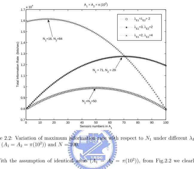
(25) is labeled as “Maximum Information Rate Deployment”. This deployment can be applied to the applications of rescuing the survivals form the wild fires, flooding regions, in cases where there are many regions to be observed. In these applications we don’t consider the critical issue of energy constrain which pose significant problem of network lifetime, since we only consider the importance of information and extend the coverage as large as possible to obtain the maximum information.. 2.3. Analysis of MIRD. In this section we we analyze the performance of our derivations with the parameters listed below:. E l r Ai Ni N λEi. Initial Energy of a sensor packet size of each event sensing range & transmitting range area of i-th region number of sensors deployed in i-th region total number of sensors event occurring rate of the i-th region. 1000 J 20 bits 1 m m2. 1/m2 /sec. Table 2.1: Parameters used in the analyses.. From (2.13) and (2.14) we obtain the optimal value of N1 and N2 to maximize I(N1 , N2 ). We can verify this derivation through Fig.2.2. It clearly depicts the variation of the total information rate I(N1 , N2 ) as a function of N1 with respect to different λE1 and λE2 when the areas of A1 and A2 are fixed and identical(A1 = A2 = π(102 )). Those arrows indicate the optimal deployment of N1 and N2 to obtain maximum information rate. We can observe that the total information rate increases as N1 increases from 0 towards the optimal value, where the slope of total information rate is positive and sharp initially. The total information rate would reach the maximum value where the corresponding value of N1 is the best deployment, which is exactly the value obtained from (2.13). 15.

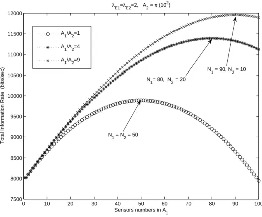
(26) A = A = π (102). 4. 1.7. 1. x 10. 2. λE1=λE2= 2. 1.6. λE1=3, λE2=2. Total Information Rate (bits/sec). 1.5. λE1=2, λE2=4. N1=16, N2=84. 1.4. 1.3. 1.2 N = 71, N = 29 1. 2. 1.1. 1. 0.9 N =N =50 1. 2. 0.8. 0.7. 0. 10. 20. 30. 40 50 60 Sensors numbers in A. 70. 80. 90. 100. 1. Figure 2.2: Variation of maximum information rate with respect to N1 under different λE , while (A1 = A2 = π(102 )) and N = 100. With the assumption of identical areas (A1 = A2 = π(102 )), from Fig.2.2 we clearly obtain a sense of putting more sensors in the area with larger λE if maximum information rate is desired. This is consistent with our intuition since more sensors in the area with larger λE would receive more information. For example, if λE1 = 3 and λE2 = 2, the optimal value of N1 is 71, that is larger than N2 = 29. Notice that when λE1 = λE2 = 2, we get N1 = N2 = 50, fa1 = fa2 = 0.3935; when λE1 = 3, λE2 = 2, we get N1 = 71, fa1 = 0.5084 and N2 = 29, fa2 = 0.2517; whenλE1 = 2 and λE2 = 4, we get N1 = 16, fa1 = 0.1479 and N2 = 84, fa2 = 0.5683. After examining the variation of I(N1 , N2 ) while λE1 differs with λE2 and A1 A2 are identical, we then study the variation of I(N1 , N2 ) if A1 and A2 are varying, λE1 and λE2 are identical. Fig.2.3 depicts the variation of I(N1 , N2 ) as a function of N1 with respect to different area ratios A1 /A2 = m. We assume λE1 = λE2 = 2‘ and A2 = π ∗ (102 ), and vary. 16.

(27) the ratio m to see the variation of I(N1 , N2 ). The result coincides with our intuition that we should put more sensors in the larger area to obtain more information. From (2.4) we know A1 and A2 are related to area coverage fa1 and fa2 , respectively, through the parameters D1 and D2 . It implies that by putting more sensors in the area, we could obtain more information while better area coverage fa is achieved. λ =λ =2, A = π (102) E1. E2. 2. 12000. A /A =1. 11500. 1. 2. A /A =4 1. 2. 11000 Total Information Rate (bits/sec). A1/A2=9 N1 = 90, N2 = 10. 10500. N1= 80, N2 = 20. 10000. 9500. N1 = N2 = 50. 9000. 8500. 8000. 7500. 0. 10. 20. 30. 40 50 60 Sensors numbers in A. 70. 80. 90. 100. 1. Figure 2.3: Variation of maximum total information rate with respect to N1 for different areas of A1 /A2 where λE1 = λE2 = 2, N = 100. Comparing Fig.2.3 with Fig.2.2, we conclude that variation of λE is more critical than variation of area, since a slight change in λE would cause a significant change of N1 and N2 . Notice that when A1 = A2 = π(102 ) and λE1 = λE2 = 2, the optimal deployment is N1 = N2 = 50, fa1 = fa2 = 0.3935 ; when A1 = 4 · A2 and λE1 = λE2 = 2, we get N1 = 80, fa1 = 0.1813 and N2 = 20, fa2 = 0.1813; when A1 = 9 · A2 and λE1 = λE2 = 2, we get N1 = 90, fa1 = 0.0952 and N2 = 10, fa2 = 0.0952, which indicates that if λE1 = λE2 , the optimal deployment is the number of sensors that makes both fa1 and fa2 the same.. 17.

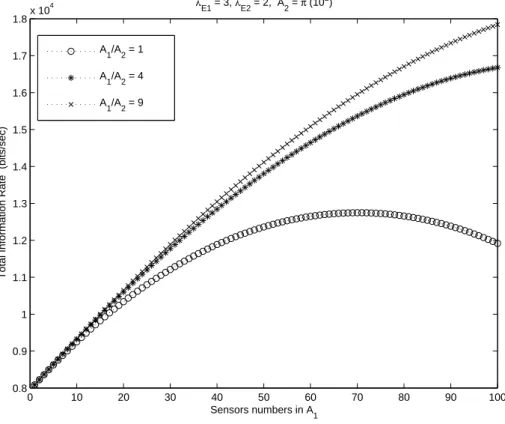
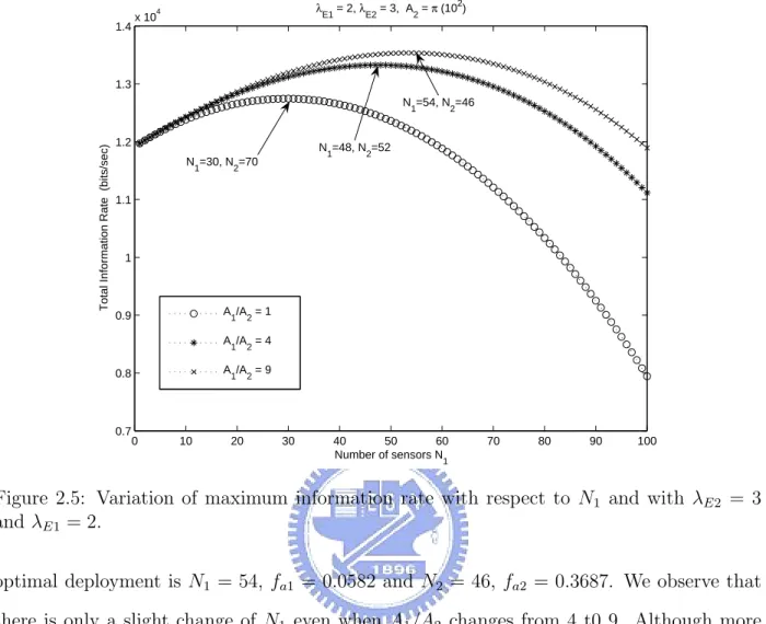
(28) From the results of Fig.2.2 and Fig.2.3, we should have an appreciation of deploying more sensors in the region which either has a larger λE or a larger area, hence area and λE can be considered as two critical factors in determining the optimum value of N1 and N2 . We keep some parameters in Fig. 2.3, i.e., A1 /A2 = m, m = 1, 4, 9, but change λE1 to be 3 in Fig. 2.4. Since A1 and λ1 are larger than A2 and λ2 , respectively, we would put more sensors in A1 . In the case of m = 4 and m = 9, even if we put all the sensors N = 100 in A1 , the slope of total information rate still positive, which means N1 has not reached the optimal value yet even if N1 = N . λ. 4. 1.8. E1. x 10. = 3, λ. E2. = 2, A = π (102) 2. A1/A2 = 1. 1.7. A1/A2 = 4. Total Information Rate (bits/sec). 1.6. A1/A2 = 9. 1.5. 1.4. 1.3. 1.2. 1.1. 1. 0.9. 0.8. 0. 10. 20. 30. 40 50 60 Sensors numbers in A1. 70. 80. 90. 100. Figure 2.4: Variation of maximum information rate with respect to N1 and with λE1 = 3, λE2 = 2, N = 100. What if we let λE2 = 3 and λE1 = 2 while A1 /A2 = 1, 4, 9? We can see the result in Fig.2.5. When λE2 = 3, λE1 = 2, A2 = π(102 ) and A1/A2 = 1, the optimal deployment is N1 = 30, fa1 = 0.2592 and N2 = 70, fa2 = 0.5034; when A1 /A2 = 4, the optimal deployment is N1 = 48, fa1 = 0.1131 and N2 = 52, fa2 = 0.4055; when A1 /A2 = 9, the. 18.

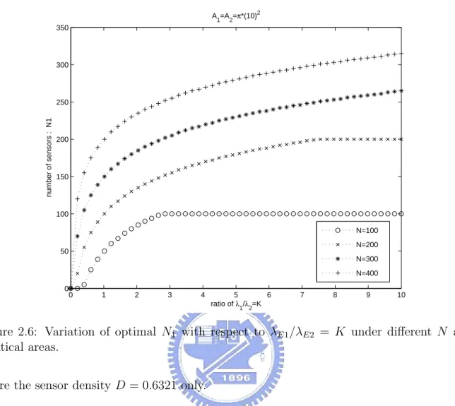
(29) λ. 4. 1.4. E1. x 10. = 2, λ. E2. = 3, A = π (102) 2. 1.3 N =54, N =46. Total Information Rate (bits/sec). 1. 1.2. 2. N1=48, N2=52. N1=30, N2=70 1.1. 1. A1/A2 = 1. 0.9. A /A = 4 1. 0.8. 0.7. 2. A /A = 9 1. 0. 10. 20. 2. 30. 40 50 60 Number of sensors N. 70. 80. 90. 100. 1. Figure 2.5: Variation of maximum information rate with respect to N1 and with λE2 = 3 and λE1 = 2. optimal deployment is N1 = 54, fa1 = 0.0582 and N2 = 46, fa2 = 0.3687. We observe that there is only a slight change of N1 even when A1 /A2 changes from 4 t0 9. Although more sensors should be put in the larger area while λE1 = λE2 , here the numbers are less than those in Fig. 2.3. By observing the variation of fa1 and fa2 in both Fig. 2.3 and Fig. 2.5, we conclude that the effect of λE is critical when fa is relatively small, and is irrelevant when fa is relatively large. We can verify this conclusion in later discussion. Now we examine the optimal value of N1 with respect to the ratio of λE when areas are identical and fixed. In Fig.2.6 we assume A1 = A2 , and vary the ratio of λ1 /λ2 = K while N could be 100, 200, 300 and 400. We see that the optimal value of N1 increases as the ratio λ1 /λ2 = K increases, and eventually N1 = N at some critical value of K. Namely, even if we put all the N sensors in one area, it doesn’t achieve enough coverage of the area yet to obtain information. For example, when N = 100, we obtain N1 = 100 at λE1 /λE2 = 2.9,. 19.

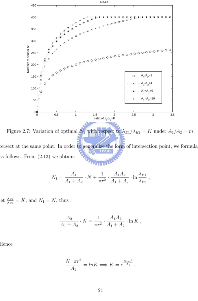
(30) A =A =π*(10)2 1. 2. 350. 300. number of sensors : N1. 250. 200. 150. 100 N=100 N=200. 50. N=300 N=400 0. 0. 1. 2. 3. 4. 5 6 ratio of λ /λ =K 1. 7. 8. 9. 10. 2. Figure 2.6: Variation of optimal N1 with respect to λE1 /λE2 = K under different N and identical areas. where the sensor density D = 0.6321 only. In Fig. 2.6, N acts like a DC component for it shifts the curves upwards or downwards but does not change the shape, as we can see in the cases of N = 300, when we deploy N1 = 250 in A1 and the corresponding fa1 is 0.9179; when N = 400, we deploy N1 = 300 in A1 and the corresponding fa1 is 0.9502, which indicates an enough area coverage is achieved to obtain most of the information. To examine the effect of λE in detail, we vary both λE and area to see the variation of optimal N1 . In Fig.2.7 we assume N = 400, A1 /A2 = m, m = 1, 4, 9, 16 and λE1 /λE2 = K. We observe that the curve reaches to the limitation of N quickly, thus the effect of λE is critical when fa is relatively small. Here we obtain the same conclusion again. In Fig.2.8, we assume N = 200 is fixed and let A2 /A1 = m and λE1 /λE2 = K, which is a little bit different from the case in Fig. 2.7. Surprisingly we observe that all the curves in20.

(31) N=400 450. 400. 350. Number of sensor N1. 300. 250. 200. A1/A2=1. 150. A1/A2=4 100. A1=A2=9 A1=A2=16. 50. 0. 0. 0.5. 1. 1.5 2 ratio of λ /λ =K 1. 2.5. 3. 3.5. 2. Figure 2.7: Variation of optimal N1 with respect to λE1 /λE2 = K under A1 /A2 = m. tersect at the same point. In order to generalize the form of intersection point, we formulate as follows. From (2.13) we obtain:. N1 =. let. λE1 λE2. A1 1 A1 A2 λE1 ·N + 2 · · ln , A1 + A2 πr A1 + A2 λE2. = K, and N1 = N , thus : 1 A1 A2 A2 ·N = 2 · · ln K , A1 + A2 πr A1 + A2. Hence : N ·πr 2 N · πr2 = lnK =⇒ K = e A1 . A1. 21.

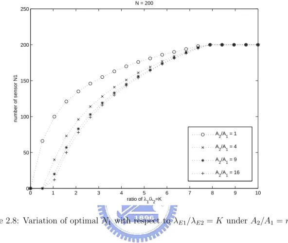
(32) which is independent of A2 /A1 = m. Therefore the intersection point is determined once A1 is determined. N = 200 250. number of sensor N1. 200. 150. 100 A2/A1 = 1 A2/A1 = 4. 50. A2/A1 = 9 A2/A1 = 16 0. 0. 1. 2. 3. 4. 5 6 ratio of λ /λ =K 1. 7. 8. 9. 10. 2. Figure 2.8: Variation of optimal N1 with respect to λE1 /λE2 = K under A2 /A1 = m.. 22.

(33) Chapter 3 Maximum Information Capacity Deployment In the previous chapter, we propose the “Maximum Information Rate Deployment”(MIRD) method for optimal sensor deployment in two areas. This method doesn’t consider the issue of energy constraint, for the objective is to obtain maximum information rate at some instant of time, thus energy consumption is completely ignored. Without lose of generality, now consider the situation : given two regions A1 and A2 , each region has its own area and event occurring rate, then how to deploy sensors in each region to obtain the maximum information capacity within the network lifetime? To deal with this issue, we first introduce the formulation of energy consumption in each transmission. Next, we formulate the relationship between energy consumption and network lifetime in a probability sense, thereby the total generated information capacity during the network lifetime period is determined. In short, through the combination of network lifetime and the “Maximum Information Capacity Deployment”(MICD), we can determine the optimal number of sensors to be deployed in each region.. 3.1. Network lifetime and information capacity. The idea behind our analyses of network lifetime is quite simple. We assume every sensor has the same initial energy E and define one transmission of an event as “one round”. Each 23.

(34) round would consume the same energy Eevent , then the number of rounds that one sensor can last is simply determined by Rounds = E/Eevent . The detail analyses starts from this simple assumption. In our work, we only discuss communication energy consumption. We do not include the energy loss of sensing here. The reason is that energy loss of sensing depends heavily on the specific application. Nevertheless, such energy loss can be easily integrated into the equations once the sensing energy model of specific application is defined. The first order model of energy consumption presented in [7] is used here. In this model Eelec = 50nJ/bit is the energy dissipated to active the transmitter or receiver circuitry and ²amp = 10pJ/bit/m2 for the transmit amplifier to deliver each bit. Thus we can get the energy consumption to transmit a k -bit packet to distance d , denoted as ET x (k, d), and the energy to receive the same packet, denoted as ERx (k, d), as follows :. ET x (k, d) = Eelec ∗ k + ²amp ∗ k ∗ d2 ,. (3.1). ERx (k, d) = Eelec ∗ k .. (3.2). We assume the transmission range of each sensor is r , which is the same as the sensing range. Then, we can simplify 3.1 as :. ET x (k, r) = KT x ∗ k ,. where KT x = Eelec + ²amp ∗ r2 . Hence, the energy consumption of a sensor on receiving l bits from the distant d and transmit k bits to the distant r can be computed as follows:. 24.

(35) ET x (k, r) + ERx (l, d) = Eelec ∗ k + ²amp ∗ k ∗ r2 + Eelec ∗ l. = KT x ∗ k + Eelec ∗ l .. (3.3). Since we adopt the random deployment of Poisson Point Process under Boolean Sensing Model, it is reasonable and straightforward to assume all sensors are identical. Specifically, we further assume only one sink node exists to collect the information and the rest are all identical sensors with same sensor parameters and functionalities. In a wireless sensor network, the sensor located far away from the sink node would transmit data to the sink node by means of multi-hop communication. Therefore, the sensors closer to the sink node will have to transmit not only their own sensing data, which is defined as the “Originating traffic”, but also relayed data of the other nodes, being termed as the “Relaying traffic”. As a result, the initial energy of these sensors will be used up the earliest among all sensors, since their traffic load is heavier than the other sensors. Thus, in such a random deployed wireless sensor network, we focus on the region R having area πr2 around the location of sink node, which is called the “inner circle”. If all the sensors deployed in the inner circle, called inner sensors, use up their initial energy, there will be no sensors to relay the information obtained from outer sensors to sink node. The time period when all the inner sensors use up their energy is therefore defined as the network lifetime for the wireless sensor network of concern. Here are some implicit assumptions to simplify the network lifetime analysis. Firstly, the traffic load from outer sensors to be relayed to sink node is evenly divided by sensors deployed in the inner circle R, which implies some ideal routing protocol is in place. Secondly, we assume the packet size of each event l is small enough and sensors can use any level of power to complete the transmission. Finally, the sensed outer information to be relayed is proportional to the outer area (Ai − πr2 ) · fai and is independent of the number of sensors 25.

(36) deployed in the outer region. To begin with, we consider the following situation : there are two regions to be monitored, which have area size A1 , A2 and event occurring rate λE1 , λE2 , respectively. In general, we assume that there are N1 sensors in A1 , N2 sensors in A2 and take s sensors in the inner circle of A1 , w sensors in the inner circle of A2 . Without lose of generality, we discuss the case of A1 first, and then it is easy to obtain similar result of A2 . Since there are s sensors in the inner circle of A1 , hence (N1 − s) sensors are in the outer region (A1 − π · r2 ). From previous results, the averaged traffic to be relayed by s inner sensors to the sink node is expressed as follows : Ireceive,s|A1 = λE1 · l · (A1 − πr2 ) · fa1,s , where 2. fa1,s = 1 − e(−Douter,s ·πr ) , and Douter,s =. N1 − s . A1 − πr2. The information to be transmitted by the s inner sensors per unit time can be denoted as :. Itransmit,s|A1 = [πr2 + (A1 − πr2 )fa1,s ] · λE1 · l .. (3.4). Therefore, the energy consumption of the s inner sensors can be computed as :. Ereceive,s|A1 +Etransmit,s|A1 = λE1 ·l ·(A1 −πr2 )·fa1,s ·Eelec +[πr2 +(A1 −πr2 )fa1,s ]·λE1 ·l ·Ktx , (3.5). Assume that every sensor has identical initial energy E and the energy consumption can 26.

(37) be evenly divided by s inner sensors, we define a parameter named Rounds(s) which is the network lifetime time that s sensors can last before their total energy s · E be used up. Thus Rounds(s) is written as :. Rounds(s) =. =. s·E Ereceive,s + Etransmit,s s·E . λE1 · l · (A1 − πr2 ) · fa1,s · Eelec + [πr2 + (A1 − πr2 )fa1,s ] · λE1 · l · Ktx. (3.6). The network lifetime of N1 is therefore determined by Rounds(s). From (3.4) and (3.6), the total information capacity that the sink node of A1 can receive from s inner sensors through the network lifetime is :. Itotal,s|A1 = Rounds(s) · Itransmit,s|A1 =. [πr2 + (A − πr2 )fa1,s ] · λE1 · l · s · E . λE1 · l · (A − πr2 ) · fa1,s · Eelec + [πr2 + (A − πr2 )fa1,s ] · λE1 · l · Ktx. (3.7). Similarly, we define the network lifetime of A2 to be Rounds(w), expressed as :. 27.

(38) Rounds(w) =. =. w·E Ereceive,w + Etransmit,w. λE2 · l · (A2 −. πr2 ). w·E , · fa2,w · Eelec + [πr2 + (A2 − πr2 )fa2,w ] · λE2 · l · Ktx. (3.8). and the total information capacity that the sink node of A2 can receive from w inner sensors through the network lifetime is :. Itotal,w|A2 = Rounds(w) · Itransmit,w|A2 =. [πr2 + (A2 − πr2 )fa2,w ] · λE2 · l · (w · E) . λE2 · l · (A2 − πr2 ) · fa2,w · Eelec + [πr2 + (A2 − πr2 )fa2,w ] · λE2 · l · Ktx. (3.9). Since we observe two regions to obtain desired information, we consider A1 and A2 as two sub-networks of the whole network. Thus it is straightforward to define the network lifetime of the whole network as :. Rounds = min{Rounds(s), Rounds(w)} ,. (3.10). which means the shorter one of Rounds(s) and Rounds(w) would dominate the network lifetime. When either of these two sub-networks run out of its energy in the inner circle, it stops gathering data from the environment. Since information is the main concern of the 28.

(39) discussion, it doesn’t matter whether another sub-network is working or not, hence (3.10) is a reasonable definition of network lifetime of the whole network. From the above discussion, the total information capacity of the whole network can be formulated as follows:. Itotal|(s,w) = Itotal,s|A1 + Itotal,w|A2 = Rounds · Itransmit,s|A1 + Rounds · Itransmit,w|A2 ,. (3.11). where the Rounds is given as (3.10). Thus, we obtain the total information capacity when there are s sensors in the inner circle of A1 and w sensors in the inner circle of A2 . Recall that we assume all the sensors are deployed in the area by the Poisson Point Process, we can compute the probability of s sensors deployed in the inner circle of A1 , and the probability of w sensors deployed in the inner circle of A2 , and through the concept of probability we can obtain the average total information capacity. From Sec.2.1.3, we can compute the probability of s sensors in the inner circle of A1 when there are N1 sensors deployed in the area A1 , given as :. P (N (A) = s|N1 ) = e(−D1 ·A) ·. (D1 · A)s , s!. (3.12). where A = πr2 and D1 = N1 /A1 . Next, the probability of w sensors located in the inner circle of A2 is:. P (N (A) = w|N2 ) = e(−D2 ·A) ·. where again A = πr2 while D2 = N2 /A2 . 29. (D2 · A)w , w!. (3.13).

(40) As (3.12) and (3.13) are independent, the probability of obtaining Itotal(s,w) in (3.11) can be expressed as :. P (Itotal|(s,w) ) = P (N (A) = s|N1 ) · P (N (A) = w|N2 ) .. (3.14). We observe that s and w are variables which can vary from 0 to N1 and from 0 to N2 respectively, thus if N1 and N2 are specified, the expected total information capacity is formulated as:. E[Itotal ] = E[Itotal|(s,w) ]. =. X. Itotal|(s,w) · P (Itotal|(s,w) ). s,w. =. N1 X N2 X. P (N (A) = s|N1 ) · P (N (A) = w|N2 ) · Itotal|(s,w) .. (3.15). s=0 w=0. Consequently, we can apply (3.15) to estimate the total information capacity for a particular (N1 , N2 ) and then look for the optimum deployment where E[Itotal ] is maximum.. 30.

(41) 3.2. Simulation Results A2 = π (52), λ1 = λ2 = 2 2. A1 = π (5 ). N1 = 500. 3500. A1 = π (7.52) A1 = π (102). Total Information Capacity : E[ I total ]. 3000. 2500. N1 = 770 2000. N 1 = 870 1500. 1000. 500. 0. 0. 100. 200. 300. 400 500 600 Sensor numbers N. 700. 800. 900. 1000. 1. Figure 3.1: The effect of varying area ratio upon maximum information capacity where N = 1000. Now we have the analytical form of E[Itotal ], by MATLAB simulations we can observe the properties of E[Itotal ]. First we assume N = 1000, let λE1 = λE2 = 2 and A2 = π(52 ), A1 could be π(52 ), π(7.52 ) and π(102 ), the resulting variation of E[Itotal ] is shown in Fig. 3.1. In order to demonstrate more clearly, in Fig. 3.2 shown next page, we let A1 be π(12.52 ), π(152 ) and π(202 ) and again show the variation of E[Itotal ]. From the figures we can tell that the effect of area size is evident and significant. Since the network lifetime is determined by the number of sensors deployed in the inner circle, and the deployment follows the Poisson Point Process, we should put more sensors into the larger area to increase the probability of sensors be deployed in the inner circle. In this case, the number of sensors deployed in the inner circle can increase, so are the network lifetime and the information capacity. When we increase the number of senors in A1 , which is N1 , the number of sensors N2 is decreased, i.e. 31.

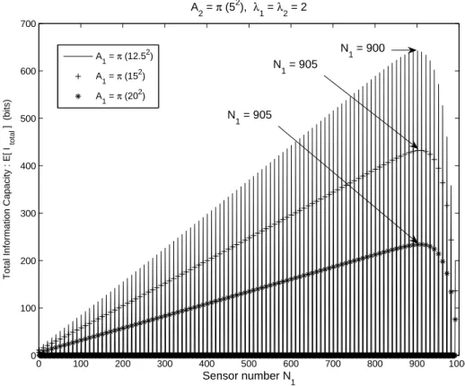
(42) we increase the network lifetime of A1 but decrease the network lifetime of A2 . The total information capacity would reach an maximum value for some optimal values of N1 and N2 , as we can see in the figures. There is an interesting observation that the effect of varying area ratio would saturate eventually, as depicted in Fig. 3.2. The reason is simple, we can’t put too few sensors in A2 , that would cause the network lifetime of A2 be too short. Since very few sensors would be deployed in the inner circle of A2 , the lifetime of the whole network will be short as well. Thus there exists a threshold of saturation. When optimal deployment of N1 reaches this threshold, it would remain the same but the total information capacity decreases. For example, for the case A1 = π(152 ) and A1 = π(202 ) in Fig. 3.2, the optimal N1 for both cases are the same, but the total informal capacity decreases as A1 increases. 2. A2 = π (5 ), λ1 = λ2 = 2 700. N1 = 900. A = π (12.52) 1. 600. N1 = 905. A = π (152) 1. Total Information Capacity : E[ I total ] (bits). 2. A1 = π (20 ). N1 = 905. 500. 400. 300. 200. 100. 0. 0. 100. 200. 300. 400. 500. 600. 700. 800. 900. 1000. Sensor number N. 1. Figure 3.2: The effect of varying area ratio upon maximum information capacity where N = 1000. After examining the effect of area upon total information capacity, now we fix the area A1 , A2 and vary λE to see the effect of λE upon total information capacity, the result is shown 32.

(43) A = A = π (52), λ = 2 1. 2. 2. 4000 λ1 = 2 λ1 = 6. 3500. N1 = 775. N = 705. N1 = 500. 1. λ1 = 10. Total Information Capacity : E[ I total ]. 3000. 2500. 2000. 1500. 1000. 500. 0. 0. 100. 200. 300. 400 500 600 Sensor numbers N. 700. 800. 900. 1000. 1. Figure 3.3: The effect of varying λE upon maximum information capacity. in Fig. 3.3. We can tell the difference between varying area ratio and varying λE ratio. The variation of total information capacity is irrelevant to the variation of λE ratio, which is due to the assumption that the traffic load is evenly divided by those sensors deployed in the inner circle. The total energy of those inner sensors implicitly imply the total information capacity that the sink node can receive during the network lifetime. When λE is larger, the energy consumption is larger, which leads to a shorter network lifetime, and vice versa. In either case the total information capacity is the same, although the optimal values of N1 and N2 varied with different λE ratio. Hence the conclusion here is that the maximum total information capacity is irrelevant to variation of λE ratio, only the area ratio would affect the total information capacity.. 33.

(44) 3.3. Searching Algorithm for Optimal Deployment. Here we introduce an algorithm to search for the optimal value of N1 , and then N2 is therefore determined by N2 = N − N1 . The detailed MATLAB algorithm is listed in Appendix A. We start from the concept of expected value, and by Dichotomy we can converge our searching to the optimal value. From the definition of network lifetime of (3.10), we have an idea of that the optimal value of N1 occurs when Rounds(s) = Rounds(w), that is because if either one of them is bigger, assume Rounds(s) is bigger than Rounds(w), it implies that we should take some sensors from A1 and deploy them into A2 to prolong the lifetime Rounds(w) in the probability sense. From the idea described above, we first examine the initial deployment, which is the expected value of sensors to be deployed in the inner circle of each area. For example, in A1 , the expected number of sensors to be deployed in the inner circle can be expressed as :. E[s] =. X · πr2 . A1. (3.16). Next, the expected number of sensors to be deployed in the inner circle of A2 is :. E[w] =. (N − X) · πr2 . A2. (3.17). The initial deployment can be determined from (3.16) and (3.17), i.e., E[s] = E[w],given as :. X=. A1 ·N . A1 + A2. (3.18). After obtaining X we can compute E[Itotal ] for the cases of X − 1, X and X + 1, respectively.. 34.

(45) This is because, from the observations of the simulation results of MICD, the maximum value of N1 occurs at the point that the slope changes from positive to negative. Since it is not possible to determine the derivative of E[Itotal ] and X is a discrete value, hence we compute E[Itotal ] for the cases of X − 1, X and X + 1 for obtaining the slope. Here we use the simplest method of Dichotomy to approach the optimal value from the initial deployment X, i.e., if E[Itotal ] of X + 1 is greater than E[Itotal ] of X, and E[Itotal ] of X is greater than E[Itotal ] of X − 1, the slope of E[Itotal ] at X is positive, which implies we should put more sensors to obtain a larger E[Itotal ]. Thus, the optimal value certainly exists in the interval [X, N ]. We set an variable named of f set to be (N − X)/2, and by examining the slope at Y = X + (N − X)/2, we can determine whether the optimal value lies in the interval [X, Y ] or [Y, N ]. Namely, if the slope at Y is positive, then the optimal value exists in the interval [Y, N ]; if it is negative, the optimal value appears in the interval [X, Y ]. Assuming that the optimal value exists in the interval [X, Y ], then we set the value of of f set to be :. of f set =. Y −X . 2. (3.19). Repeat the same process and then we can narrow the searching interval, eventually the optimal value is obtained. The detail algorithm is shown in Appendix A. By using this algorithm, we can examine the effects of varying ratio of area or λE . The results are shown below.. Fig. 3.4 depicts the optimal value of N1 with respect to the ratio of A1 /A2 = K while λE1 and λE2 are identical and fixed, and N = 1000. It is seen that, when K is small, we should put plenty of sensors to the larger area even if there is only a slight change of area ratio, which implies that in the Maximum Information Capacity Deployment, area is the critical concern. Moreover, the optimal value of N1 saturates when A1 /A2 is large. 35.

(46) A = π (52), λ 2. E1. =λ. E2. =2. 1000. 900. 800. K = 6.25, N = 907 Optimal number of sensors N1. 1. 700. K = 4, N = 867. 600. 1. 500. K=2.25 , N1 = 774 400. 300. K=1, N = 500 1. 200. 100. 0. 0. 2. 4. 6. 8 A /A =K 1. 10. 12. 14. 16. 2. Figure 3.4: Optimal N1 of MICD under varying area ratio. Fig. 3.5 depicts the optimal value of N1 with respect to the ratio of λE1 /λE2 = m while A1 = A2 , and N = 1000. We can tell that the optimal value of N1 is less sensitive to the variation of λE ratio on comparing Fig. 3.4 and Fig. 3.5. The curve of Fig. 3.4 increases sharply and reach the saturation state relatively quickly, while the curve of Fig. 3.5 increases slowly and smoothly, and doesn’t reach saturation even when λE1 /λE2 = m is very large. The effect could be seen more clearly in Fig. 3.6.. 36.

(47) λ. E2. = 2, A = A = π (52) 1. 2. 900. 850. Optimal number of sensors N1. 800. 750. 700. 650. 600. 550. 500. 0. 2. 4. 6. λ /λ E1. 8. E2. 10. 12. 14. 16. =m. Figure 3.5: Optimal N1 of MICD under varying λE ratio. 950. 900. Optimal number of sensors N1. 850. 800. 750. 700. 650. 600. 550. 500. 0. 2. 4. 6. 8 10 λE1/λE2 = A1/A2 = r. 12. 14. 16. Figure 3.6: The comparison of Optimal N1 with respect to varying λE ratio and area ratio. 37.

(48) Chapter 4 Generalized Maximum Information Rate Deployment 4.1. Generalized form of MIRD. We can generalize the deployment problem of Chapter 2 to K regions, and each region has its own area Ak and average event occurring rate λEk , respectively. The deployment problem can be formulated as :        . N. =. K X. Ni ,. i=1.        I(N1 , . . . , Nk ) =. K X. (4.1) fai · (λEi · Ai · l) ,. i=1. where   fai = . 2. 1 − e−Di πr , (4.2). Di =. Ni Ai. i = 1, . . . , k .. The general form of the number of sensors Ni of the ith region Ai for the K-area case can be computed as :. 38.

(49) K X. I(N1 , . . . , NK ) =. fai · (λEi · Ai · l) =. i=1. Let Xi = Ai λEi l and Ri =. πr2 , Ai. K X. N. − Ai πr2. (1 − e. i. ) · (λEi · Ai · l) .. i=1. then. I(N1 , . . . , NK ) =. K X. Xi · (1 − e−Ni Ri ) ,. i=1. By applying the method of Lagrange Multiplier to this optimization problem, we formulate the objective function as :. g(N1 , . . . , NK ) = I(N1 , . . . , NK ) + λ(N − N1 − N2 − . . . − NK ) ,. (4.3). where λ is an unknown scaler to be determined. The maximum value of I(N1 , . . . , NK ) ∂g occurs when = 0, j = 1, . . . , K, written as : ∂Nj. ∂g ∂Nj. = Xj Rj e−Nj Rj − λ = 0. =⇒ λ = Xj Rj e−Nj Rj ,. j = 1, . . . , K .. (4.4). Thus. Nj =. 1 [ ln(Xj Rj ) − ln λ ] . Rj. Since. N1 + . . . + NK = N , 39. (4.5).

(50) hence. Pk j=1. =⇒. 1 [ ln(Xj Rj ) − ln λ ] = N Rj. ln λ =. S2 − N , S1. (4.6). where S1 and S2 are two constants, calculated as :. k k X 1 1 X = 2 Aj , R πr j j=1 j=1. S1 =. k X ln(Rj Xj ). S2 =. j=1. Rj. k 1 X = Aj ln(πr2 λEj l) . πr2 j=1. From (4.5) and (4.6), we get. Nj. 1 = Rj. ·. N S2 + ln(Xj Rj ) − S1 S1. ¸. k X. =. Aj Aj ln(πr2 λEj l) − 2 · 2 πr πr. Ai ln(πr2 λEj l). i=1 k X. + Ai. i=1. Ai k X. j=1. 40. (4.7). Ai. i=1. Let αj = πr2 λEj l, then (4.7) can be simplified as   k X      Aj ln αj       Aj Aj  j=1 Nj = k N + ln α − , j k  πr2  X X      Aj Aj      j=1. ·N .. (4.8).

(51) Here we show a 3-dimensional plot as shown in Fig. 4.1 to demonstrate that the total information rate indeed reaches maximum value at the exact values of sensors estimated from (4.8).. 2400. Total Information Capacity. 2300. X: 7 Y: 7 Z: 2302. 2200 2100 2000 1900 1800 1700 25 20. 25 15. 20 15. 10 10. 5 Sensor numbers N2. 5 0. 0. Sensor numbers N1. Figure 4.1: 3-areas case of MIRD, where N = 21, λE1 = λE2 = λE3 = 2, A1 = A2 = A3 = π(52 ).. 4.2. Analyses of 3-area case of MIRD. Here we show some conceptual analyses of 3-area case of MIRD. First we consider the third area having fixed parameters, thus there are four modes of the this area : (1). A3 is large and λE3 is small; (2). A3 is small and λE3 is large; (3). Both A3 and λE3 are large; (4). Both A3 and λE4 are small. Under these four modes of the third area, first we fix the value of λE1 and λE2 to be 2, and vary the ratio of A2 /A1 = K, A1 = π(52 ) to see the effect of area upon optimal deployment of N1 , N2 and N3 , when N = 600. The results are shown in the next few pages. First we compare Fig. 4.2a with Fig. 4.2b, the difference is A3 = π(102 ) in Fig. 4.2a being larger than A3 = π(2.52 ) in Fig. 4.2b. We observe that the variation of N3 in Fig. 4.2a 41.

(52) is larger than that in Fig. 4.2b, we should put more sensors to N3 when A3 is large in order to increase the area coverage fa3 and obtain more information. Since λE1 = λE2 = λE3 = 2, N2 would be larger than N3 when A2 is larger than A3 . A = π (102),λ 3. E3. = 2, A = π (52), λ 1. E1. =λ. E2. = 2, N = 600.. 500 N1. 450. N2. 400 Number of sensors N1,N2 and N3.. N3 350. 300. 250. 200. 150. 100. 50. 0. 0. 1. 2. 3. 4. 5 A /A =K 2. 6. 7. 8. 9. 10. 1. (a). Figure 4.2: Optimal deployment of N1 , N2 and N3 with respect to variation of area ratio : A2 /A1 = K while there are four modes of the third area. Then we compare Fig. 4.2a with Fig. 4.2d, the difference is that λE3 = 10 in Fig. 4.2d, which is larger than λE3 = 2 in Fig. 4.2a, while A3 = π(102 ). We can see that even A2 grows to very large, we still put large number of sensors to N3 , which is caused by the large area of A3 with large λE3 , as it’s more efficient to put more sensors in A3 to obtain more information. Now we compare Fig. 4.2c with Fig. 4.2b, with A3 = π(2.52 ) and λE3 = 10 in Fig. 4.2c and λE3 = 2 in Fig. 4.2b. Here the curve of N3 is similar to each other, which due to A3 = π(2.52 ) is small, we need only few sensors in A3 to achieve enough area coverage fa3 . For example, when N3 = 50 and A3 = π(2.52 ), fa3 = 0.9997, when N3 = 25, fa3 = 0.9817. 42.

(53) A = π (2.52), λ 3. E3. = 2, A = π (52), λ 1. E1. =λ. E2. = 2, N = 600.. 600. Number of sensors N1,N2 and N3.. 500. 400. 300. 200. 100. 0. 0. 1. 2. 3. 4. 5 A /A =K 2. 6. 7. 8. 9. 10. 8. 9. 10. 1. (b) A = π (2.52),λ 3. E3. = 10, A = π (52), λ 1. E1. =λ. E2. = 2, N = 600.. 600. Number of sensors N1,N2 and N3.. 500. 400. 300. 200. 100. 0. 0. 1. 2. 3. 4. 5 A2/A1=K. 6. 7. (c). Figure 4.2: Optimal deployment of N1 , N2 and N3 with respect to A2 /A1 = K while there are four modes of the third area. 43.

(54) A = π (102),λ 3. E3. = 10, A = π (52), λ 1. E1. =λ. E2. = 2, N = 600.. 600. Number of sensors N1,N2 and N3.. 500. 400. 300. 200. 100. 0. 0. 1. 2. 3. 4. 5 A /A =K 2. 6. 7. 8. 9. 10. 1. (d) A = π (52), λ. 4. 9. 1. x 10. E1. =λ. E2. = 2, N = 600. Maximum total Information Rate (bits/sec). 8. 7. A = π (102), λ 3. E3. =2. A3 = π (2.52), λE3 = 2. 6. A3 = π (102), λE3 = 10. 5. A3 = π (2.52), λE3 = 10 4. 3. 2. 1. 0. 0. 1. 2. 3. 4. 5 A2/A1=K. 6. 7. 8. 9. 10. (e) Maximum total information rate with corresponding optimal deployment with respect to A2 /A1 = K.. Figure 4.2: Optimal deployment of N1 , N2 and N3 with respect to A2 /A1 = K while there are four modes of the third area. 44.

(55) In the end we depict the variation of maximum information rate with respect to A2 /A1 = K under four modes of the third area in Fig. 4.2e. We can see that the highest curve is the mode of both λE3 and A3 are large, and the lowest curve is the mode of both λE3 and A3 are small, which is reasonable result based on our previous discussion. After complete the discussion about the effect of area, now we fix the areas of A1 and A2 to be π(52 ), and vary λE2 /λE1 = m to see the effect of λE upon optimal deployment and maximum total information rate, while there are again four modes of the third area. Firstly we compare Fig. 4.3a with Fig. 4.3b, we observe that the curves of N1 , N2 and N3 are flat and there is little difference whether λE3 is large or small when determining the optimal deployment. This is due to the area coverage fa is enough, for example, when N3 = 400 and A3 = π(102 ), fa3 = 0.9817; when N1 = 100 and A1 = π(52 ), fa1 = 0.9817; while λE2 /λE1 = m is growing, we should take some senors from N3 , N1 to N2 . A = π (102), λ =2, λ 3. E3. E1. = 2, A = A = π (52), N = 600. 1. 2. 600. N1 500. N2 N. Number of sensors N1, N2 and N3. 3. 400. 300. 200. 100. 0. 0. 1. 2. 3. 4. 5 λE2/λE1= m. 6. 7. 8. 9. 10. (a). Figure 4.3: Optimal deployment of N1 , N2 and N3 with respect to variation of λE2 /λE1 = m while there are four modes of the third area. 45.

(56) Comparing Fig. 4.3b with Fig. 4.3c, we observe that N3 in Fig. 4.3b is around 4 times than that in Fig. 4.3c. It’s reasonable that we should put more sensors in the larger area. Notice that when A3 = π(102 ) and N3 = 400, then fa3 = 0.9834; when A3 = π(2.52 ) and N3 = 80, then fa3 = 0.9999. Now comparing Fig. 4.3c with Fig. 4.3d, the difference is λE3 = 10 in Fig. 4.3c and λE3 = 2 in Fig. 4.3d. It seen that the curves of optimal deployment are very similar, which implies that the effect of λE becomes irrelevant to optimal deployment when area coverage is large enough. Notice that when A3 = π(2.52 ) and N3 = 80, fa3 = 0.9999; when A2 = π(52 ) and N2 = 220, fa2 = 0.9998, then we can get a better understanding of this conclusion. We demonstrate the curves of maximum total information rate under corresponding optimal deployment in Fig. 4.3e. We find that the curves are straight lines, which differ from the case previously discussed, that is due to the area coverage fa is an exponential form with respect to the information rate, while that of λE is a linear form. From the discussions of varying area and varying λE in 3-area case of MIRD, we can conclude that area is a critical concern to the optimal multi-area WSN deployment, which implies that when the total number of sensors N are not enough for every region to achieve sufficient coverage, the non-linear effect of exponential form is critical. From Fig. 4.2a and Fig. 4.2d, Fig. 4.3c and Fig. 4.3d, we conclude that the effect of λE is critical when fa is small, and becomes irrelevant when fa is sufficient large, which is the same conclusion obtained in the analyses of 2-area MIRD. There are too many scenarios that can be discussed, for example we can vary N to see what is the resulting effect. This is somehow too complicated to be investigated, thus here we only discuss some simple scenarios, but the basic principle still holds.. 46.

(57) A = π (102), λ =10, λ 3. E3. E1. = 2, A = A = π (52), N = 600. 1. 2. 600. Number of sensors N1, N2 and N3. 500. 400. 300. 200. 100. 0. 0. 1. 2. 3. 4. 5 λ /λ = m E2. 6. 7. 8. 9. 10. 8. 9. 10. E1. (b) A = π (2.52), λ =10, λ 3. E3. E1. = 2, A = A = π (52), N = 600. 1. 2. 5 λE2/λE1= m. 6. 600. Number of sensors N1, N2 and N3. 500. 400. 300. 200. 100. 0. 0. 1. 2. 3. 4. 7. (c). Figure 4.3: Optimal deployment of N1 , N2 and N3 with respect to variation of λE2 /λE1 = m while there are four modes of the third area. 47.

(58) A = π (2.52), λ =2, λ 3. E3. E1. = 2, A = A = π (52), N = 600. 1. 2. 600. Number of sensors N1, N2 and N3. 500. 400. 300. 200. 100. 0. 0. 1. 2. 3. 4. 5 λ /λ = m E2. 6. 7. 8. 9. 10. E1. (d) A = π (102),λ. 4. 10. 3. x 10. E3. = 10, A =A =π (52), λ 1. 2. E1. = 2, N = 600. 9. Maximum total Information Rate (bits/sec). 8 A = π (2.52), λ = 10 3. 7. E3. 2. A3 = π (10 ), λE3= 10. 6. A3 = π (102), λE3= 2. 5. A3 = π (2.52), λE3= 2. 4. 3. 2. 1. 0. 0. 1. 2. 3. 4. 5 λE2/λE1=m. 6. 7. 8. 9. 10. (e) Maximum total information rate with corresponding optimal deployment with respect to λE2 /λE1 = m.. Figure 4.3: Optimal deployment of N1 , N2 and N3 with respect to λE2 /λE1 = m while there are four modes of the third area. 48.

(59) Chapter 5 Conclusion In this work we introduce the Maximum Information Rate Deployment(MIRD) and the Maximum Information Capacity Deployment(MICD) for multi-area WSNs. We assume the sensors are randomly deployed by the 2-dimensional Poisson Point Process, and the occurrence of event follows the Poisson Process. In the MIRD, we don’t consider the issue of energy consumption and network lifetime, but focus on how to deploy the sensors in multiple areas to obtain the maximum information rate. Through detailed analyses of 2-area MIRD, we should put more sensors into the larger area in order to achieve better coverage fa , and should put more sensors in the area with larger λE . Still we conclude that the effect of λE is a critical issue of MIRD when area coverage fa is not enough. Later we discuss the energy consumption and define the network lifetime of multi-area WSNs, and obtain the deployment when maximum information capacity is desired. Through detailed simulation results, we conclude that area is the most critical issue of MICD, since the network lifetime is determined by those sensors around the sink node and more sensors would increase the probability of sensors to be deployed around the sink node. Finally in the analyses of 3-area case of MIRD, we apply Lagrange Multiplier to obtain the optimal sensor deployment. It becomes more complicated when determining the optimal deployment if there are more areas, however the conclusions obtained from 2-area MIRD still holds. 49.

(60) Appendix A Searching Algorithm for Optimal Deployment of MICD We express the searching algorithm as the follows :. //Initial deployment get expected number of sensors N_1 : N1 = X; //determine initial offset offset = \frac{(N-N1)}{2};. while{} x = E[I_{total}(N_1-1)]; y = E[I_{total}(N_1)]; z = E[I_{total}(N_1+1)];. // slope at N1 is positive if y<z && y>x N_1 = N_1 + offset; offset = offset/2; 50. X/{A1}=(N-X)/A2;.

(61) if offset < 1 offset = 1 end. // slope at N1 is negative elseif y>z && y<x N_1 = N_1 - offset; offset = offset/2; if offset < 1 offset = 1 end. // This is the case we are looking for, // slope change from positive to negative and optimal value appears elseif y>z && y>x N1 break; end end. 51.