Active noise cancellation by using the linear quadratic Gaussian
independent modal space control
Mingsian R. Bai and Chifong Shieh
Department of Mechanical Engineering, National Chiao Tung University, 1001 Ta Hsueh Road, Hsinchu 30050, Taiwan, Republic of China
(Received 1 August 1994; accepted for publication 25 November 1994)
The objective of this study is to develop an active noise controller based on optimal control approaches for enclosed Gaussian noise fields. By independent modal space control, the individual mode in the acoustic field is suppressed by the corresponding modal control exerted by loudspeakers. The formulation of the modal controller is considerably simplified because modal coupling is neglected. For the Gaussian noises considered in this study, the linear quadratic Gaussian algorithm in conjunction with the Kalman-Bucy filter is employed to perform state feedback and estimation. The developed controller is validated by simulations for a duct and a rectangular room. The results indicate that the technique will yield significant noise reduction if one uses the same number of controlled modes, microphones, and loudspeakers. Satisfactory performance is possible if one carefully avoids placing microphones and loudspeakers at the nodal points.
PACS numbers: 43.20.Ks, 43.50.Ki
INTRODUCTION
Noise control for enclosed acoustic fields falls into two categories: the passive approach and the active approach. The former is conventional and is based on some well-
developed
design
methods
such
as the acoustic
filter
theory.
•
On the other
hand,
active
noise
control
(ANC)
2 is based
on a
principle that one artificially generates an antifield to de- structively interfere with the undesirable noise field. It pro- vides certain advantages over the passive approach. These attractive features include improved low-frequency perfor- mance, reduction of size and weight, zero back pressure, and programmable flexibility of design. Advances are being made toward developing a commercial hybrid active- passive noise controller in which the low-frequency attenua- tion is provided by an active system, while the high- frequency attenuation is provided by passive hardware. There are many applications of the ANC technique, includ- ing silencers for gas pipelines, noise cancelers for air condi- tioning systems, mufflers for internal combustion engines,
noise
attenuators
for vehicle
or airplane
cabins,
and
so
forth.
2
This study focuses primarily on the development of an ANC technique for enclosed Gaussian noise fields, based on
the linear
quadratic
Gaussian
(LQG)
3 algorithm
in conjunc-
tion with independent
modal
space
control
(IMSC).
4'5
The
analysis is motivated by the formulation of the large space
structure
(LSS)
6'7 since
both
systems
are of the distributed
type and have an infinite number of degrees of freedom. The control actions for LSS may be taken in the actual space as well as in the modal space. The latter approach is adopted in this study due to the simplicity of the controller design. This simplicity stems from uncoupling a continuous system (de- scribed by a partial differential equation) into a set of simple oscillators (described by modal ordinary differential equa- tions) via orthogonality of eigenfunctions. In theory, one can control the entire system by controlling the infinite number
of modes of the system. In practice, one is only able to con- trol low-frequency modes, e.g., below the Schroeder's cutoff frequency, where modal decomposition is meaningful. The applications of modal control can be found in many areas in structural dynamics, such as beam vibration, flo•w•-dnduced
vibration,
airfoil
fluttering,
and
so forth.
6-•ø
Among the modal control techniques, the IMSC seeks to control the individual mode of a continuous system by modal controls by neglecting modal coupling. This provides a re- markable reduction of problem size in controller design. However, IMSC requires distributed types of sensors and
actuators
which
are essentially
free of spillover
effects.
5'•
This poses a problem because the most commonly used transducers in acoustic applications are discrete types, e.g., microphones and loudspeakers. Thus a suitable approxima- tion scheme must be taken to represent the measurement and control actions of the acoustic field by using a finite number of discrete sensors and actuators.
In the design of the modal controller, two techniques are available to accomplish the state feedback. One method is based on pole allocation and the other is based on linear
quadratic
(LQ) optimal
control.
•2-•4
In this
research,
the lat-
ter is adopted because it not only admits a reasonable bal- ance between the control error and control effort but also yields a stable control system. In addition, if the control sys- tem of interest is subjected to stochastic excitations, then the LQG algorithm should be employed. In viewing that the LMS algorithm and its variants are prevailing methods in the
ANC community,
2 the LQG-IMSC
technique
proposed
in
this paper provides a useful alternative in attenuating noises in enclosures.
A duct and a rectangular room are selected as test cases in a simulation to investigate the effects of various control parameters. The results indicate that the developed technique will yield significant noise reduction if the same number of controlled modes, microphones, and loudspeakers are em-
v(o,o
x=0 x=/ x=L=/+0.6a (a) Speaker Microphone (b)FIG. 1. (a) Schematic diagram of an open-ended duct of length 2 m, driven
by a rigid piston; (b) configuration of the LQG-IMSC system for the duct.
ployed. Satisfactory performance is possible if one carefully avoids placing actuators and sensors at the nodal points.
I. THEORY AND METHOD
A. Modal equations of the acoustic fields
In this section, modal equations of a duct and a rectan- gular room are derived by using the orthogonality of eigen- functions. For the duct case of Fig. 1, it is assumed that one end of the duct is driven by a rigid piston of surface velocity v(O,t) and the other end is left open with radiation imped- ance z n . The surface velocity is assumed to be Gaussian white. Since only the plane waves below the cutoff fre- quency are of interest, the duct field is essentially reduced into a one-dimensional problem. The governing equation of the duct field is •5
1 02p(x,t) 02p(x,t)
cW
= f ( x,
t ) ,
( )
subject to the boundary conditions
8p(O,t) Ov(O,t)
•= 8x -p •= 8t -pa(O,t), (2)
p(l,t)=ZnV(l,t), (3)
and some initial conditions, where p(x,t) is the sound pres- sure in the duct, a(0,t) is the surface acceleration of the piston, f(x,t) is the control function, c is the speed of sound, and p is the density of medium. The open end of the duct can be approximated by a pressure-released boundary with the effective length of the duct L increased by 0.6x the radius a
(for an unflanged
circular
duct).
•5 That
is,
p(x,t)=O at x=L(=l+O.6a). (4)
Solving the eigenvalue problem associated with Eqs. (1), (2), and (4) yields the eigenvalues
I I LQO-•SC Controller
• ß
Speaker
'Microphone-;•f ß Primary noise source
FIG. 2. Configuration of the LQG-IMSC system for a 1 m X 1.5 m x2 m rectangular room containing a monopole noise source.
kr=[(rc/2L)(2r-1)] 2, r=l,2,...,m
(5) and the normalized eigenfunctionscos
(6)Since the orthogonal eigenfunctions •br(x) form a complete set, the sound pressure p(x,t) and the control function f(x,t) can be expanded as follows:
p(x,t) = • p•(t) rk•(x),
r=l
(7)
f(x,t)
= • •-•
r=lf•(t)
qb•(x),
(8) where P r(t) is the modal pressure and fr(t) is the modal control function. Conversely, pr(t) and f•(t) can be ex-tracted
by modal
filtering:
•6
p•(t)= •-•
p(x,t)
qb•(x)dx,
(9)f •(t) = f(x,t) rkr(x)dx. (10)
With some manipulations, the modal equation for the duct
can
thus
be expressed
as
•6
d2pr(t)
d2t
•+
krC2pr(t)=
pc2a(t)+ fr(t),
r= 1,2,...,o•, (11)
where the first term at the right-hand side represents the modal excitation due to the primary noise.
On the other hand, assume that a rectangular room of
dimensions
L x, L y, and
L z , as shown
in Fig. 2, is bounded
by rigid walls. A monopole source with known volume ve- locity per unit volume q(t) is present in the room. Hence the governing equation of the problem is
0
1 02p(x,t)
_ V2p(x,t)
+ p q(t)6(X_Xs)+f(x,t)
c-• Ot • - •
subject to the rigid-walled boundary conditions
Op
OX(O,y
'z,t)=0,
•xx
(Lx'Y'Z't)=O
'Op
(x,O,z,t)
=0, Op
Oy
•yy
(x,Ly
,z,t)=0,
(13)
OP
Oz '
(x,y
O,t)=O
' Op
•zz
(x'y'Lz't)=O'
and some initial conditions, where x-(x,y,z) and xs=(x s ,ys ,%) are the position vectors of the field point and the source point, respectively, f(x,t) is the control function, and 8(x-x s) is the three-dimensional Dirac delta function. Solving the eigenvalue problem of Eqs. (12) and (13) yields the eigenvalues
Xr= -E-x/
+
+ -E-z/
(14)and the normalized eigenfunctions
•r(X)=C xLyLz
cos'
Lx cos
Ly cos
Lz '
05)
where
nx,ny,nz=O,1,2,...,
o• and r-l,2,...?. Note that the
subscript
r is being.•.used
as a triple index, so that
r=(nx,ny,nz).
•en, Similar
to the duct
case,
the sound
pressure p(x,t). and the control hnction f(x,t) can be ex- panded on the basis of the eigenfunctions
p(x,t)
= • pr(t)qbr(X),
r=l (16)f(x,t) = • 1/C2fr(t)qbr(X).
r=l (17)Using
the
orthog,onality
of eigenfunctions,
the
modal
pres-
sure
and
the moii•l
control
function
can
be obtained
by the
modal filter
fv
pr(t)
= • P(X,t)qbr(x)dx,
(18)fr(t)
= f /(x,t)qbr(x)dx,
(19) where V is the domain of the volume integral for the room. Thus the partial differential equation in Eq. (12) can be un-coupled
into
the
following
modal
equations:
16
d2pr(t)
O
dt
•+
•'rC2pr(t)=P
• q(t)qbr(Xs)+
fr(t)'
r= 1,2,...,m. (20)
It can be observed from Eqs. (11) and (20) that the modal equations of the one-dimensional duct problem and the 2666 J. Acoust. Soc. Am., Vol. 97, No. 5, Pt. 1, May 1995
three-dimensional room problem are essentially of the same form except for the definitions of the eigenfunctions and the
source terms.
B. Control by state feedback and estimation
Continuous systems such as the aforementioned duct and room have an infinite number of natural modes. This requires an infinite-order controller if global control is de- sired. In practice, modal truncation is often necessary to in-
clude
only the predominant
low-order
modes
(say,
n modes)
in order for the controller to be implementable. This leads to a finite number of modal equations
d2pr(t) •
d2
•
+ XrC2pr(
t) =
pc2a(
t) + f r(
t),
r= 1,2,...,n (21)
for the duct and
d2pr(t)
09
'
dt
•+
XrC2pr(t)=P
• q(t)qbr(Xs)+
fr(t)'
r= 1,2,...,n (22)
for the rectangular room. Either of the modal equations in Eqs. (21) and (22) can be expressed as the following modal state form (for the rth mode only):
ir(t) = Arxr(t) + Brfr(t) + Wrl (t),
Y
r(t)
= Crxr(t)
+ Drwr2
(t),
(23)
where
Xr=[rOrPr(t)Pr(t)]
T is the rth modal
state
vector,
•Or
- c •r is the rth nature
frequency,
fr(t) is the modal
control function for the loudspeakers, and y r(t) is the modal output measured by the microphones. Note that the first com- ponent of the state vector is given as rOrPr(t), rather than just pr(t) for better conditioning of matrices. This is a necessary step to avoid numerical problems in solving the Riccatti equation. The coefficient matrices in the modal state equa- tion are accordingly defined as
0
Dr=[0 1 ].
(-O r
gr •
1]'
Cr=[
1/to
r 0],
(24)
The matrices Wrl(t ) and Wr2(t ) representing the noise terms of the source and the sensor, respectively, in the modal space are defined as Wrl(t) = 0
2x• pc2a(
t)
[ 0 ]
Wrl(t)=
p •-•
q(t)qbr(Xs)
for the duct or (25)
for the room and (26)
Wr2(t)-- 0
Wr2(t) for both the duct and the room, (27) where Wr2(t) is the intensity of the modal sensor noise. It can be proved that the modal state equations are both con-
trollable
and
observable.
5 In the study,
the source
noise
and
the sensor noise are assumed to be zero mean and Gaussian
white. That is, the covariance matrix of the noise terms sat-
isfies
Wrl(tl)
E Wr2(tl
) [WrTl(t2)
Wr•(t2)
] =¾r(tl)•5(tl--t2),
(28) where the intensity matrix of the joint process ¾r(t) is de- fined as
¾rll(t)
Vr(t)-
VrT21(t)
with ¾r12(t) ¾r22(t) (29) Vrl I = o o 0 Vr• Vrl 2 = Vr21 =o o]
0 Vrl 2 ' Vr2 2 =o o]
0 Vr22 'Here, the stochastic process is said to be nonsingular if
Vr22>0
and uncorrelated
if Vr•2=0.
3 In our case,
we re-
stricted ourselves to the controller design for the nonsingular and uncorrelated white noise only.
According to the method of IMSC, state feedback is carried out for each individual mode of the physical plant. Hence the modal control function of the rth mode is gener- ated as a linear combination of the modal pressure and its
first time derivative, i.e.,
f r( t) = GrXr = -- grPr( t) - hrt3r( t). (30) One question remaining is how to determine the modal gains gr and h r in Eq. (30). Two of the commonly used
techniques
are pole allocation
and optimal
control.
•2-14
In
this research, the latter method is adopted because it not only admits a reasonable balance between the control error and control energy but also yields a stable control system. Since the acoustic system in our case is subjected to stochastic excitations, a more general optimal control approach, the
LQG algorithm,
is employed.
TM Note, however,
that the
presence of the Gaussian white noise in the system does not
alter the form of solution as its deterministic LQ version,
except to increase the minimal value of the optimal
criterion.
3 Because
modal
coupling
is neglected,
the global
optimum can be obtained by minimizing the following per- formance index for individual modes:
Jr=E
( T
X r Qrxr + Rrf r)dt + XrPlrX2
T
r ,0
(31)
where E{ ) denotes the expected value, Qr=diag{Qr,Qr}, Qr >•0, Rr>O, Plr is a real symmetric positive semidefinite matrix, and t o and t• are the initial time and the final time, respectively. The scalars Q r and R r stipulate the relative im- portance of the control error and control energy. A large Qr :Rr ratio corresponds to expensive control, while a small
Q r :Rr ratio corresponds to cheap control. Minimization of the performance index in Eq. (31) amounts to regulating the system response as close to the zero state while, on the other hand, keeping the expenditure of control energy as low as possible.
The optimal modal control gains gr and h r in accord with the performance index in Eq. (31) can be calculated by
Gr =R 1 T
•- BrPr,where
Pr is the solution
of the Riccati
equation
3
(32)
_ •}r=
gr I _ PrBrTR
•-1
BrPr
+ ArTpr
+ PrAr
'
(33)subject to the final condition Plr(tl)=Plr, where I is a 2X2 identity matrix. In this study, only the steady-state case is of concern, i.e., •r=0, and Eq. (33) reduces to the algebraic Riccati equation. Solving the algebraic Riccati equation leads to the following closed-form solutions:
2 'Jr-
R r) - 1ar (Dr]}
1/2
P r l l = R r { 2 (Dr
[ 4 (Dr2
+ ( (D
r
--
,
2+Rr)-lRr (Dr],
Pr12=Pr21=Rr[
q(Dr2
+ ( (Dr
--
(34)Pr22=Rr{ 2[•Or
--2+( 2 -1R
(Dr R r) r]+ 2•o•-
1[
(Dr
2 .}_
((Dr2Rr)-
1Rr]3/2
} 1/2.
The modal LQG regulator should work very well when the information of states is fully available. In reality, how- ever, the information of states is generally incomplete or in- accurate. This calls for the need of a modal state observer
that
is based
on the Kalman-Bucy
filter
3
•r(t) = Ar•r(t)
+ arf r + Kr[y
r(t) - Ci.•r(t)],
(35)
where
•r(t) = [(Drier(t) t•r(t)] T is the estimated
modal
state vector. Consider the state estimation error
er(t)=•r(t)--Xr(t ). (36)
The optimization problem amounts to finding the modal gain matrix K r such that the weighted mean-square estimation
error
E{err(t)Wrer(t)}
is minimized,
where
Wr is a symmet-
ric and positive definite matrix. The optimal solution of the matrix K r (which is independent of the matrix Wr) can be
calculated
by
3
Kr(t)=Qr(t)Crr(t)V•-2•(t),
t>•to,
(37)
where Q r is the solution of the Riccati equation
(•r= Vrlli_
QrCr
T - 1
V•22CrQr
+ QrArT+
ArQr
.
(38)
Since
only
the steady-state
case
is of interest
((•r=0), the
closed-form solution of Qr simply reads
Qrll Vrll{2(Dr[4(Dr2+(
= (Dr2
+ Vrll)-1
Vrll (Dr]__ }1/2,
=
2+Vrll)-lVrl -(Dr],
(39)
Qr12 Vrll[4(Dr2'}-((Dr
1
2.}_( 2Vr
1 )-lVrl ]
Qr22= Vrl l{- 2[ (Dr (Dr 1 12.}_( 2
-1
3/2}1/2.
'}-
2(D•-
1[
(Dr
(DrVr ) Vrll]11
•m• Actuators
I
:"1
Acoustic
p(x,O
.I Sensors
I
Discretization regulator Interpolation
ii
I
...
I .
I
I I Inverse
• • ModM
state I K•m•
modM
L• ModM
L I
[
•mod• filter••
feedback
l½,,,,
I state
obsever
[e,•
filter I-
I
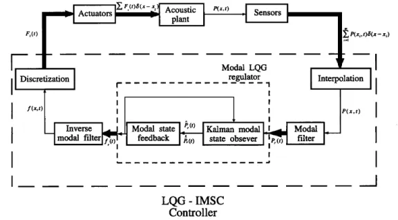
LQG- IMSC Controller
FIG. 3. Overall •C system framework based on the LQG-IMSC technique.
C. Discrete sensors and actuators
The ideal IMSC formulation requires distributed sensors and actuators. If this requirement is satisfied, then every mode of the continuous system can be controlled and no
spillover
will occur.
5 In practical
implementation
of the
ANC
system, only discrete loudspeakers and microphones are available from the state of art. This produces spillover prob- 1. ems, as will be discussed in the end of this section.
First, the numerical aspect concerned with discrete sen- sors is discussed. Since in practice sound pressure can only be measured by a finite number of discrete microphones, an appropriate interpolation scheme must be used to accurately reconstruct the original acoustic field, i.e.,
m
p(x,t)= • Si(x)p(xi,
t ),
i=1
(40)
where/5 (x,t) is the interpolated sound pressure, p (xi ,t) are the sound pressures measured by the finite number of dis- crete microphones, and S i(x) are interpolation functions.
Several
options
of interpolation
functions
are
available.
•7 In
this study, the interpolation function based on the Rayleigh- Ritz method is employed to reconstruct the acoustic field because it makes use of the eigenfunctions that provide a better approximation of the system characteristicsß According to the Rayleigh-Ritz method, the sound pressure p(x,t) can be expressed as the linear combination of eigenfunctions
n
p(x,t)= • ar(t)(•r(X),
r=l
(41)
where ar(t ) are the modal, coordinates. Therefore substitut- ing rn measured sound-pressure data {p(xi,t)}, i= 1,2,...,rn into Eq. (41) gives the following linear equations'
p(x•,t) p(x2, t) ß ß ß ß ß ß ß ß ß p(Xm, t) 4,2(x,) '" (x2) >2(x2) ... a•(t) a2(t) ß X , an(t)
or, written more compactly,
•>n (Xm)
(42)
{p (xb t)} = [• ]{ar(t)}, (43)
where [•] is an m Xn real matrix that contains spatially
sampled
eigenfunctions.
The coefficients
{ar(t)} can be ob-
tained by pseudoinverting Eq. (43)'
{ar(t)} = [• ]+ {p (xb
t) }.
(44)Note that the pseudoinverse becomes the actual inverse for a nonsingular [•] if the same number of microphones is used as the controlled modes. Substituting Eq. (44) into Eq. (41) yields
m n
P(X,t)
= • • [r!P]r•Ckr(X)p(xi,
t),
i=1 r=l
(45)
where
[•]r• stands
for the
ri component
of the
matrix
[•]+.
Comparing Eq. (45) with Eq. (40) indicates that the interpo- lation function based on the Rayleigh-Ritz method takes the
following form:
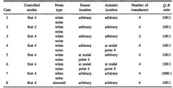
TABLE I. Simulation cases for the duct.
Controlled Noise Sensor Actuator Number of Q :R
Case modes type location location transducers ratio
1 first 4 white arbitrary arbitrary 4 100:1
noise
2 first 2 white arbitrary arbitrary 4 100:1
noise
3 first 4 white arbitrary arbitrary 2 100:1
noise
4 first 4 white arbitrary at nodal 4 100:1
noise point 4
5 first 4 white at nodal arbitrary 4 100:1
noise point 4
6 first 4 white at nodal at nodal 4 100:1
noise point 4 point 4
7 first 4 white arbitrary arbitrary 4 1000:1
noise
8 first 4 sinusoid arbitrary arbitrary 4 100:1
n
Si(x)
= • [(I)]r•r(X)-
r=l
(46)
Parallel to the above-mentioned discrete sensor problem, a finite number of discrete loudspeakers employed to control the acoustic fields renders a similar approximation problem. If one uses as many loudspeakers as microphones and allo- cates the loudspeakers at the points x i, i= 1,2,...,rn, the associated control function can be written as
m
f(x,t) = • Fi(t) 8(x- xi),
i=1
(47)
where Fi(t ) are the amplitudes of the discrete control func- tions produced by the ith loudspeaker. This corresponds to the modal control functions
m
fr(t) = • qbr(xi)Fi(t),
r = 1,2,...,n,
(48)
i=1
which can also be written in the following matrix form:
{fr(t) } = [ • ]{Fi(t)}, (49)
where [cI)] has the same form as in Eq. (43). In IMSC, the modal control functions are determined first and the actual
control functions are then computed. Hence we need the in- verse relation to that given by Eq. (49), i.e.,
{Fi(t)}=[•]+{f r(t)},
(5O)where
[cI)]
+ is the pseudoinverse
of [cI)].
It should
be noted
that a pseudoinverse is not an actual inverse and the above process does not yield genuine IMSC. To design a control function for each controlled mode independently as required by IMSC, one must have as many loudspeakers and micro- phones as the controlled modes, m-n, in which case
[cI)]
+ = [cI)]
-•. The effect
of this
point
will be explored
further
in Sec. II.
A final note regarding spillover effects is in order. It can be shown in IMSC that control spillover will not destabilize the system, although it can cause degradation in the system
performance.
5 Observation
spillover
alters
the system
eigen-
values and can possibly produce instability in the residual modes. This is particularly true if the loudspeakers and mi-
crophones
are not collocated.
5
The overall ANC system framework based on the LQG- IMSC technique is depicted in Fig. 3. The sound pressure measured by the discrete microphones is interpolated, modal filtered, and fed to the modal LQG regulator. The regulator then produces optimal modal control functions that are in turn sent to the inverse modal filter and discretized into ac-
TABLE II. Simulation cases for the rectangular room.
Controlled Sensor Actuator Number of Q :R
Case modes location location transducers ratio
1 first 4 arbitrary 2 first 2 arbitrary 3 first 4 arbitrary 4 first 4 arbitrary 5 first 4 at nodal plane (0,1,1) 6 first 4 at nodal plane (0,1,1) arbitrary 4 100:1 arbitrary 4 100:1 arbitrary 2 100:1 at nodal 4 100:1 plane (0,1,1) arbitrary 4 100:1 at nodal plane (0,1,1) 4 100:1
TABLE III. Modal frequencies of the acoustic field inside the duct.
Mode index Modal frequency (Hz)
i 43.1 2 129.4 3 215.7 4 302.0 5 388.3 6 474.6 7 560.9 8 647.2
tual control functions for the discrete loudspeakers. The en- tire process forms a closed-loop modal control system for noise cancellation.
II. NUMERICAL SIMULATION
Simulation cases are designed to investigate the effects of control parameters on the LQG-IMSC technique. The pa- rameters for the simulation include the type of primary noise,
number of controlled modes, number of sensors and actua- tors, location of sensors and actuators, and the Q:R ratio.
The simulation cases for the duct and the room are shown in Tables I and II, respectively. Although mode shapes are glo- bal properties and the modal control technique should pre- sumably achieve global control, the results presented below show the power spectra (in decibels) calculated by averaging the sound pressure only at the sensor locations. This is not only because of the limitation of computer facility but also because we are more interested in creating quiet zones, e.g., the vicinity of the passenger's heads in a car cabin, which is in fact the only possibility in practical applications at high-
frequency
ranges.
2 The power
spectrum
calculation
is based
on 20 records of 1024 time samples for FFT. In each of the following cases, the simulation parameters will be changed one at a time to investigate the performance of the LQG- IMSC controller. 8o[- •. 70 v
• so
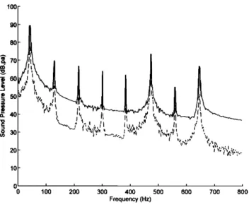
.e 5o a. 40 e- o 30- 2O 10 0 0 100 200 300 400 500 600 700 8 0 Frequency (Hz)FIG. 5. Response spectrum of case 2 for the duct problem (• uncon-
trolled field; --- controlled field). Four microphones and four loudspeakers
are employed to control the first two modes. The microphones and loud- speakers are collocated at x =0.25, 0.75, 1.25, and 1.75 m, respectively. The
Q:R ratio is selected to be 100:1.
A. The duct case
The LQG-IMSC technique is first applied to a duct of length 2 m and radius 0.1 m whose natural frequencies asso- ciated with the first eight acoustic modes are listed in Table III. In case 1, four loudspeakers and four microphones are
used to control the first four modes with Q:R=100:l. The
primary noise is zero-mean Gaussian white noise. This is
chosen as the reference case. In the simulation result of Fig.
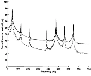
4, significant reduction (maximum 20 dB) of the sound- pressure spectrum can be observed in the frequency range of interest (800 Hz). It is interesting to note that all of the first eight modes are affected by not only the control action (for the first four modes) but also the spillover effect.
In case 2, the controller performance is investigated if
lOO
70so
5O 40 30 2O 10 0 0 i i i i 100 200 300 400 500 600 700 800 Frequency (Hz)FIG. 4. Response spectrum of case 1 for the duct problem ( uncon-
trolled field; --- controlled field). Four microphones and four loudspeakers
are employed to control the first four modes. The microphones and loud-
speakers are collocated at x=0.25, 0.75, 1.25, and 1.75 m, respectively. The Q:R ratio is selected to be 100:1.
2670 J. Acoust. Soc. Am., Vol. 97, No. 5, Pt. 1, May 1995
,oo[
•. 70'%.,',
,;,
, il . ,..., .., ,_.. a- 40- P, o• • ,• .... 20 ]0 0 i i i i i i i 0 1 O0 200 300 400 500 (500 700 8•)0 Frequency (Hz)FIG. 6. Response spectrum of case 3 for the duct problem ( uncon-
trolled field; --- controlled field). Two microphones and two loudspeakers
are employed to control the first four modes. The microphones and loud- speakers are collocated at x=0.25, 0.75, 1.25, and 1.75 m, respectively. The
Q:R ratio is selected to be 100:1.
,00[
• 7o't
,0
,,-.. /i,, ,
'•
....
• 30 20 10 0 i i 0 i00 200 300 400 500 600 700 800 Frequency (Hz)FIG. 7. Response spectrum of case 4 for the duct problem. ( uncon- trolled field; --- controlled field). Four microphones and four loudspeakers are employed to control the first four modes. The microphones are located at x=0.25, 0.75, 1.25, and 1.75 m, respectively. The loudspeakers are collo- cated at x =0.86 m, which is the nodal point of the fourth mode. The Q :R
ratio is selected to be 100:1. 100 90 80 70 50
40-
•
,,
...,, •,_..7•
•o
?'-'¾
.?-
lO 0 & i i i i i 0 100 200 300 400 500 600 700 800 Erequen• (Hz)FIG. 9. Response spectrum of case 6 for the duct problem ( uncon- trolled field; --- controlled field). Four microphones and four loudspeakers are employed to control the first four modes. The microphones and loud- speakers are collocated at x = 0.86 m, which is the nodal point of the fourth
mode. The Q:R ratio is selected to be 100:1.
only the first two modes are controlled. As shown in Fig. 5, excellent noise reduction of the first two modes is obtained, while the third mode and the fourth mode remain unchhnged. The peaks of the seventh mode and the eighth mode are changed due to spillover effects.
In case 3, the number of microphones and loudspeakers is reduced to two. The simulation result is shown in Fig. 6. Comparison between the results of cases 3 and 1 suggests that satisfactory performance of the controller can be achieved if a large number of transducers are used. This not unexpected since a large number of microphones and loud- speakers provide better approximations to the distributed field as required by the IMSC formulation.
,00[
•> 60 , •' L //' R' 40 g 30 '""" ' 20 10 0 i i i i i i 0 100 200 300 400 500 600 700 800 Frequen• (Hz)FIG. 8. Response spectrum of case 5 for the duct problem ( uncon- trolled field; --- controlled field). Four microphones and four loudspeakers are employed to control the first four modes. The microphones are collo- cated at x=0.86 m, which is the nodal point of the fourth mode. The loud- speakers are located at x=0.25, 0.75, 1.25, and 1.75 m, respectively. The
Q:R ratio is selected to be 100:1.
Because the loudspeakers and microphones are of dis- crete nature, how one places these transducers is critical to the controller performance. In case 4, the effect of locations of loudspeakers is investigated. If loudspeakers are placed at the nodal point of the fourth mode, the result in Fig. 7 shows that the peak of the fourth mode has not been reduced. The fourth mode is uncontrollable by this loudspeaker arrange- ment. Conversely, in case 5, if the microphones are placed at the nodal point of the fourth mode, the result in Fig. 8 shows that no attenuation has occurred at the peak of the fourth mode. The fourth mode is unobservable by this microphone arrangement. In case 6, the microphones and loudspeakers are collocated at the nodal point of the fourth mode. It can be observed from the result in Fig. 9 that the performance is improved.
,00[
90 80• •o
• 40 '
v ....
•'..' • •,•..• •' •P' I•, •1 ,•,.20[
, ½,;..,.,',.-,::.,,
10 0 i i i i i , 0 100 200 300 400 500 600 700 800 Frequency (Hz)FIG. 10. Response spec•trum of case 7 for the duct problem ( uncon- trolled field; --- controQed field). Four microphones and four loudspeakers are employed to control the first four modes. The microphones and loud- speakers are collocated at x=0.25, 0.75, 1.25, and 1.75 m, respectiYely. The
Q:R ratio is selected to be 1000:1.
• so o,. 40 • 30 20- 0 i ! i I i i 100 200 300 400 500 600 700 800 Frequency (Hz)
FIG. 11. Response spectrum of case 8 for the duct problem ( uncon-
trolled field; --- controlled field). Four microphones and four loudspeakers
are employed to control the first four modes. The microphones and loud- speakers are collocated at x =0.25, 0.75, 1.25, and 1.75 m, respectively. The Q:R ratio is selected to be 100:1. The primary noise is the sinusoidal signal.
In case 7, the Q:R ratio is further increased to 1000:1,
while the other settings remain the same as in case 1. The result in Fig. 10 shows that larger reduction of noise level
can indeed be obtained than that of case 1. However, one
may not be able to increase the Q:R ratio indefinitely in practical implementation since this may overdrive the loud- speakers.
As can be seen in the above-mentioned cases, Gaussian
white noises can be successfully suppressed by the LQG- IMSC technique. In case 8, the primary noise is changed into sinusoidal type. The result in Fig. 11 shows that the LQG algorithm yields only limited attenuation away from the fre- quency of the sinusoid but no attenuation at the frequency of the sinusoid. This is because the sinusoidal noise is non- Gaussian type and thus the Kalman-Bucy filter does not
function
properly.
More
precisely,
the
solution
of the
Riccatti
equation based on the assumption of Gaussian noise is no longer the optimal one for the sinusoid. This implies that, for the highly correlated non-Gaussian noises, such as the sinu- soids and periodic noises, one should resort to simpler meth-
ods
like repetitive
control.
•s
B. The rectangular room case
Next, the LQG-IMSC technique is applied to a rectan-
gular room of dimensions 1 m X 1.5 m x2 m whose natural
TABLE IV. Modal frequencies of the acoustic field inside the rectangular
room.
Mode index Modal frequency (Hz)
(0,0,1) 86.3 (0,1,0) 115.0 (0,1,1) 143.8 (1,0,0) and (0,0,2) 172.6 (1,0,1) 193.0 (1,1,0) and (0,1,2) . 207.4 (1,1,1) ,. 224.7 (0,2,0) 230.1 • 70
I:L
0'•.lr•
l•
A
.-.
•
•
50I I I I ,•
100 150 200'"'
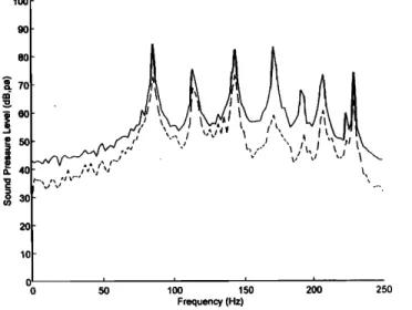
250 Frequency (Hz)FIG. 12. Response spectrum of case 1 for the rectangular room problem ( uncontrolled field; --- controlled field). Four microphones and four loudspeakers are employed to control the first four modes. The microphones
and loudspeakers are collocated at (0.1, 0.2, 0.3), (0.2, 0.7, 1.3), (0.15, 1.3, 1.6), and (0.9, 1.4, 1.9 m), respectively. The Q:R ratio is selected to be
100:1.
frequencies associated with the first eight acoustic modes are listed in Table IV. Several important parameters explored in
the duct case, such as number of controlled modes, number
of microphones and loudspeakers, and location of sensors and loudspeakers, will be revisited for the rectangular room
case.
In case 1, four loudspeakers and four microphones are used to control the first four modes of the sound field inside the rectangular room. This is used as the reference case. The simulation result in Fig. 12 shows significant noise reduction of all modes (maximum 30 dB) achieved by the LQG-IMSC technique. If four actuators are used, four modes can be c9n- trolled independently. Although more modes can be attenu- ated than expected, as demonstrated in Fig. 12, it is actually
80 •. 70 •, 50 •- 40 o 30 2O 10 0 0 i i 50 100 150 200 250 Frequency (Hz)
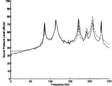
FIG. 13. Response spectrum of case 2 for the rectangular room problem
(• uncontrolled field; --- controlled field). Four microphones and four
loudspeakers are employed to control the first two modes. The microphones and loudspeakers are collocated at (0.1, 0.2, 0.3), (0.2, 0.7, 1.3), (0.15, 1.3,
1.6), and (0.9, 1.4, 1.9 m), respectively. The Q:R ratio is selected to be
100:1.
100 100 80 • 70 • 5o a. 40 (• 3o 0 I J l 0 50 100 150 200 250 Frequency (Hz)
FIG. 14. Response spectrum of case 3 for the, rectangular room problem
(• uncontrolled field; --- controlled field). Two microphones and two loudspeakers are employed to control the first four modes. The microphones
and loudspeakers are collocated at (0.1, 0.2, 0.3) and (0.2, 0.7, 1.3 m),
respectively. The Q:R ratio is selected to be 100:1.
a function of actuator locations. In case 2, if the control is
imposed on only the first two modes, the first two resonance
peaks
are significantly
attenuated,•as
shown
in Fig. 13. How-
ever, the noise level of the (1,0,1)':mode is increased because of the spillover effect.
In case 3, only two loudspeakers and two microphones are employed to control the enclosed noise field. The simu- lation result is shown in Fig. 14. In comparison with the reference case 1, less noise attenuation is obtained by using the reduced number of transducers. This situation is basically the same as that of the duct case.
In case 4, the loudspeakers are placed on the nodal plane of the (0,1,1) mode. The result in Fig. 15 shows that noise
,00[
'•. 70 v 6O ß 5013.
40
'?/%.//.-./"--
0 I I I I , 0 50 100 150 200 250 Frequency (Hz)FIG. 15. Response spectrum of case 4 for the rectangular room problem
( uncontrolled field; --- controlled field). Four microphones and four loudspeakers are employed to control the first four modes. The microphones
are located at (0.1, 0.2, 0.3), (0.2, 0.7, 1.3), (0.15, 1.3, 1.6), and (0.9, 1.4, 1.9
m), respectively. The actuators are located at (0.1, 0.75, 0.8), (0.2, 0.7, 1), (0.5, 0.75, 1), and (0.9, 1.4, 1 m), respectively, which are on the nodal plane
of mode (0,1,1). The Q:R ratio is selected to be 100:1.
80 •. 70 . 5O s. 40 • 30 0 i i i i 0 50 100 150 200 250 Frequency (Hz)
FIG. 16. Response spectrum of case 5 for the rectangular room problem (• uncontrolled field; --- controlled field). Four microphones and four loudspeakers are employed to control the first four modes. The microphones are located at (0.1, 0.75, 0.8), (0.2, 0.7, 1), (0.5, 0.75, 1), and (0.9, 1.4, 1 m), respectively, which are on the nodal plane of mode (0,1,1). The loudspeak- ers are located at (0.1, 0.2, 0.3), (0.2, 0.7, 1.3), (0.15, 1.3, 1.6), and (0.9, 1.4,
1.9 m), respectively. The Q:R ratio is selected to be 100:1.
level of the (0,1,1) mode cannot be reduced because this mode appears uncontrollable to the controller for this par- ticular loudspeaker arrangement. In case 5, the microphones are placed at the nodal plane of the (0,1,1) mode. Figure 16 shows a poor control performance and serious spillover be- cause of the incomplete microphone measurement. Similar to the duct case, if the loudspeakers and the .microphones are collocated, the control performance can be improved, as shown in Fig. 17. It can be concluded from these results of the rectangular room that similar behavior of the LQG-IMSC technique has occurred as that of the duct case. As a conse- quence, an increase of the dimensionality of the problem does not necessarily lead to an increase of the complexity of
,00[
[ 70• •o
• 50 a. 40 •o 3o i i i i 50 100 150 200 250 Frequency (Hz) 20FIG. 17. Response spectrum of case 6 for the rectangular room problem ( uncontrolled field; --- controlled field). Four microphones and four loudspeakers are employed to control the first four modes. The microphones and loudspeakers are collocated (0.1, 0.75, 0.8), (0.2, 0.7, 1), (0.5, 0.75, 1), and (0.9, 1.4, 1 m), respectively, which are on the nodal plane of mode
(0,1,1). The Q:R ratio is selected to be 100:1.
the controller formulation. Of course, this statement is true
only when the increase of the number of I/O channels in a hardware configuration required by a three-dimensional problem is not considered.
III. CONCLUSION
In this study, the LQG-IMSC algorithm is employed to
control enclosed Gaussian noise fields. In IMSC, state feed- back and estimation is carried out for each individual mode,
ß • ?.3" .
which
results
in a slmpl½.
f6rmulatlon
of controller
design.
Control gains are determined by the LQG algorithmsthat pro- vides a proper weight (depending on the power rating of the loudspeaker) between the state of disturbance and ,expendi- ture of control energy. The simulation results of a duct and a rectangular room exhibit the effectiveness of the developed active noise canceler that provides global reduction of noise level in the enclosed fields.
Although an ideal IMSC algorithm requires distributed sensors and actuators, only discrete microphones and loud- speakers can be used in the ANC application. However, the
simulation
results
indicate
that
good
performance
can
possi-
bly be achieved by using a moderate number of microphones and loudspeakers. When the number of microphones and the
number
of loudspeaker•
are both
selected
to be identical
ßto
the number
of controlled
modes,
i.e., the transformation
'/na-
trices in Eqs. (46) and (50) are both square, satisfactory con- trol performance could be obtained. Naturally, this might limit the use of IMSC when one wishes to control many modes and an exceedingly large number of transducers might
cause
a potential
problem
in practical
implemen[ation.
In ad-
dition, great care has to be taken not to plade the micro- phones and loudspeakers right at or near the nodal points.
Another
problem
that
may
arise
in using
discrei'e
types
of
sensors and actuators is the spillover effect. This undesirable phenomenon may be alleviated by collocating the micro- phones and loudspeakers. Hardware implementation based on digital signal processors to verify the observation ob- tained from this simulation is currently under way.
ACKNOWLEDGMENT
The work was supported by the National Science Coun- cil in Taiwan, Republic of China, under Project No. NSC 83-0401-E-009-024.
1M. L. Munjal, Acoustics of Ducts and Mufflers (Wiley, New York, 1977). 2p. A. Nelson and S. J. Elliott, Active Control of Sound (Academic, London,
1992).
3H. Kwakernaak and R. Sivan, Linear Optimal Control Systems (Wiley-
Interscience, New York, 1972).
4 H. 6z and L. Meirovitch, "Stochastic independent modal space control of distributed-parameter systems," J. Optimization Theory Appl. 40, 121- 154 (1983).
5L. Meirovitch, Dynamics and Control of Structures (Wiley-Interscience,
New York, 1990).
6M. J. Balas, "Trends in large space structure control theory: Fondest hope,
widest dreams," IEEE Trans. Autom. Control Ac-27, 522-535 (1982).
7 G. S. Nurre, R. S. Ryan, H. N. Scofield, and J. L. Sims, "Dynamics and
control of large space structures," J. Guidance Control Dyn. 7, 514-526 (1984).
8L. Meirovitch and H. Baruh, "Control of self-adjoint distributed param- eter systems," J. Guidance Control Dyn. 15, 60-66 (1982).
9L. Meirovitch and H. 6z, "Control of distributed gyroscopic systems,"
AIAA Pap. 78, 330-340 (1978).
løM. J. Balas, "Active control of flexible systems," J. Optimization Theory Appl. 25, 415-436 (1978).
11L. Meirovitch and L. M. Silverberg, "Globally optimal control of self-
adjoint distributed systems," Optimal Control Appl. Methods 4, 365-386 (1983). ';
12 m. J. Grimbld and M. A. Johnson, Optimal Control and Stochastic Esti- mation, Theory and Applications (Wiley, New York, 1988).
i3.A.E. Byson, Jr. and Y. C. Ho, Applied Optimal Control (Hemisphere, New York, 1981).
14 B. D. O. Anderson and J. B. Moore, Optimal Control, Linear Quadratic Methods (Prentice-Hall, Englewood Cliffs, NJ, 1990).
15A. D. Pierce, Acoustics: An Introduction to its Physical Principles and Applications (Acoustic Society of America, Woodbury, NY, 1989). 16R,. Haberman, Elementary Applied Partial Differential Equations, with
Fourier Series and Boundary Value Problems (Prentice-Hall, Englewood Cliffs, lql], 1987).
17L. Meirovitch and H. Baruh, "The implementation of modal filters for control of structures," J. Guidance Control Dyn. 8, 707-716 (1985). 18K. K. Chew and M. Tomizuka, "Steady-state and stochastic performance
of a modified discrete-time prototype repetitive controller," Trans. ASME
J. Dyn. Syst. Meas. Control 112, 35-41 (1990).