The effects of Gaussian beams on optical coherence tomography

(1)

Chun-Chu Liu

a

, Chi-Hsiang Cheng

b

, Chien-Wei Chiu

b

and I-Jen Hsu

b*

a

_{Department of Electrophysics, National Chiao Tung University, Hsinchu, 300, Taiwan,}

b

_{Department of Physics, Chung Yuan Christian University, Chungli 32023, Taiwan}

ABSTRACT

The theory of optical coherence tomography (OCT) was conventionally considered as the light beams propagating in the system to be in the forms of planar waves. However, the actual behaviors of the light beams in an OCT system are more likely to be Gaussian beams. With the consideration of the light beam passing through the focal lens in the sample arm to be a Gaussian beam, we deduced the theory of OCT in an analytic form. We also simulated and analyzed the interference signals with different positions of the photodetector and the interface in the sample as well as their transverse patterns spectrally. The results were demonstrated by experiments with a Fourier-domain OCT system.

Keywords: Gaussian beam, optical coherence tomography, interference, ultra-broadband, transverse pattern

1. INTRODUCTION

Optical coherence tomography (OCT) is a noninvasive imaging technique to extract cross-sectional information from biological tissues1, 2_{. It has been rapidly developed and is useful in biomedical applications}1-7_{. Among the alternative}

configurations of OCT systems, Fourier-domain OCT (FD-OCT) records the information as the function of frequency and obtains the structure of a tissue with Fourier transformation8-11. A typical OCT system is based on the configuration of a Michelson interferometer. The theory of OCT was conventionally considered as the light beams propagating in the system to be in the forms of planar waves. Under such an assumption, the theory of OCT is quite simple and is consistent with most of the experimental results. However, the actual behaviors of the light beams in an OCT system are more likely to be Gaussian beams12, 13_.

While considering the effects of Gaussian beams, the interference signals in an OCT system will be different to that resulting from planar waves. Furthermore, the effects will be more crucial when an ultra-broadband light source was used to achieve a high-resolution imaging, which is one of the most important issues in the current development of OCT. The problem of the larger deviation of objective lens from focal plane makes the fail description for the mirror position by the interference signals14_.

In this work, we develop the mathematical expression for the light beam from the sample arm that has the characteristics of a Gaussian beam. We calculated the interference signals received by the detector, and simulated the effects of Gaussian beam in the interference signals with the sample mirror placed at different positions deviated from the focal plane of the objective. The theoretic predictions were also demonstrated with a FD-OCT system.

2. THEORY

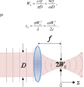
A typical OCT system is based on the configuration of a Michelson interferometer as shown in Fig. 1. The reference mirror moves longitudinally (x) and the sample mirror is put at a distance S from the focal plane of the objective lens. After reflected by the beamsplitter, the light beam propagates to and reflected by the reference mirror and finally stop at the detector with a traveling distancelR, while the optical length of sample arm is lS,

D D R R=2L +L =2(l+ f +x)+L l , (1) D D S S =2L +L =2(l+ f +S)+L l , (2)

SPIE-OSA/ Vol. 6627 66270T-1

(2)

Fig. 1. The OCT system.

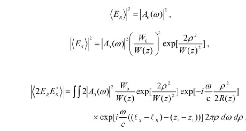
where f is the focal length of the objective lens, l is the distance between the beam splitter and focal plane, and lD is the distance from beam splitter to the detector. The required time for the sample and reference beams to travel from the beam splitter, reflected by the mirror, and finally arrived the detector are lS/c and lR/c, respectively. We suppose the light beam of the reference arm is the planar wave in the whole journey after the collimator. The wave function of a planar wave is the function of ω, z, and t,

)] ( exp[ ) ( ) , , ( z t A0 i t kz ER ω = ω ω − , (3)

where A0(ω) is the spectral amplitude and the experimental measurement is the power spectral density

2 0(ω)

A .

On the other hand, the signal of the sample arm is supposed to be a Gaussian distribution beam since it has been focused by the objective lens. One can obtain the beam waist W0 by the incident beam diameter D,

D cf D f W ω π λ 4 2 0= = , (4)

as shown in Fig.2 Rayleigh range

c W W z 2 2 0 2 0 0 ω λ π ₌ = . (5)

Fig. 2. The sample single propagates through an objective lens and focus with waist W0 at where z = 0.

SPIE-OSA/ Vol. 6627 66270T-2

(3)

While the Gaussian beam at a distance from the waist is smaller than z0, the radius of the curvature of the wavefront is

approximate to the planar wave, i.e. at waist the radius is infinite. After exceeding the Rayleigh range, the radius will gradually increase.

We set the traveling coordinate z for the sample beam at the waist as the beginning position z = 0, as shown in Fig.2, the light beam is reflected by the mirror, goes back passing the lens and splitter, and finally arrives the detector. To estimate the beam size and radius of the curvature of wavefront, we utilize the ABCD matrix,

⎟ ⎟ ⎟ ⎟ ⎠ ⎞ ⎜ ⎜ ⎜ ⎜ ⎝ ⎛ − − − + − = ⎟⎟ ⎠ ⎞ ⎜⎜ ⎝ ⎛ + ⎟⎟ ⎟ ⎠ ⎞ ⎜⎜ ⎜ ⎝ ⎛ − ⎟⎟ ⎠ ⎞ ⎜⎜ ⎝ ⎛ = ⎟⎟ ⎠ ⎞ ⎜⎜ ⎝ ⎛ f S f f LS S f f L S f f L D C B A 2 1 2 2 1 1 0 2 1 1 1 0 1 1 0 1 , (6)

with L=l+ f . We can obtain the beam size,

2 / 1 0 2 0 2 2 2 ₂ ₂ ₎ ₍ ₎ ( 2 ⎟⎟ ⎠ ⎞ ⎜⎜ ⎝ ⎛ _× + − + − ⋅ = π ω π f z z f L LS fS f c WD , (7)

and the radius of curvature of the wavefront of Gaussian beam,

2 0 2 2 0 2 2 2 ) ( ) 2 2 ( 2 ) ( ) 2 2 ( z f L f fS LS S z f L LS fS f RD ⋅ − + − − ⋅ − + − + = , (8)

at detector as shown in Fig. 3. At detector center the traveling coordinate of the sample signal is z1

D L l f S z1= 2 + + + , (9)

and deviated from the center at transverse coordinate ρi, the traveling coordinate is zi,

1 2 2 _z R R zi = i− i −ρi + . (10)

Fig. 3. The sample single propagates through an objective lens and focus with waist W0 at where z=0.

Here, we use the cylindrical coordinate, since the Gaussian beam has the cylindrical symmetry at the traversed planar. The wave function of a Gaussian laser beam wave function toward + can be express as the function of ρ, ω, z, and t, zˆ

)] ( exp[ ] ) ( 2 exp[ ] ) ( 2 exp[ ) ( ) ( ) , , , ( 2 2 2 0 0 i t kz z R c i z W z W W A t z ES ρ ω = ω ρ − ω ρ ω − . (11)

The intensity of the interference between two electric fields in Eqs. (3) and (11) is

* 2 2 2 R S S R D E E E E I = + + , (12) SPIE-OSA/ Vol. 6627 66270T-3

(4)

1500 CO 1000 ci, 500 800 850 900 950 1000 Wavelength(nm) with 2 0 2 ) (ω A ER = , ] ) ( 2 exp[ ) ( ) ( ₂ 2 2 0 2 0 2 z W z W W A ES ρ ω _⎟⎟ ⎠ ⎞ ⎜⎜ ⎝ ⎛ = , (13) and , 2 ))] ( ) (( exp[ ] ) ( 2 c exp[ ] ) ( 2 exp[ ) ( ) ( 2 2 1 2 2 2 0 2 0 * ρ ω πρ ω ρ ω ρ ω d d z z c i z R i z W z W W A E E i R S S R − − − × − =

_∫∫

l l (14)

in which we integrate with all of the frequency and the beam area over the detector. The parts of ER 2 and

2

S

E are dc signals and we only need to consider their cross-interference term ₂ *

S RE

E in Eq. (14). Here, the transverse distribution of the interference signal, i.e. the intensity in ρ direction since the signals have the cylindrical symmetry, is

. ))] ( ) (( exp[ ] ) ( 2 c exp[ ] ) ( 2 exp[ ) ( ) ( 2 2 1 2 2 2 0 2 0 * ω ω ρ ω ρ ω ρ d z z c i z R i z W z W W A E E i R S S R − − − × − =

_∫

l l (15)

3. NUMERICAL AND EXPERIMENTAL RESULTS

For comparison, we setup a Fourier Domain (FD) OCT system as Fig.1. The light source in our system is a superluminescent diode (SLD D890, Superlum Diodes Ltd.) with a spectral bandwidth of 150 nm (FWHM) centered at 890 nm as Fig. 4 and axial resolution of 3.7 µm in air. The collimated light (by an object lens: 60X, NA = 0.85, f = 2.9mm) is split half (50%) to the reference mirror and half to the reference mirror. At the sample side, a near IR achromatic doublet lens (Thorlabs, Inc.) with focal length 7.5mm makes the photon beam reflected by the sample has the character of Gaussian beam; while at the reference side, the photon beam is reflected by the mirror directly and remain to be the planar waves. Finally the interference signals are received by a spectrometer (USB2000, Ocean Optics, Inc.). The data obtained by the spectrometer are the interference intensity in frequency domain. For the time domain distribution one will need to do the Fourier transformation that we do this analysis by software LabVIEW.

Fig. 4. The spectral density distribution with the center wave length 890 nm and band width 150 nm.

SPIE-OSA/ Vol. 6627 66270T-4

(5)

1.0 0.8 = 50.6 >, 40 = 0.4 0) C 0.2 0.0 -30 -20 -10 0 10 20 30

Mirror position (6orn)

0.8 t406 0.4 5 02 S =

3Opm,f,

S90pm 0.8 00 0.4 02 ₍ p S150pm 0.8 00 0.4 02 p p 0 10 20 30 40 50 sO Mirror position (pm) 10 S2101sm 0.8 00 0.4 4, C — 02 70 80 90 100 110 120 120 130 140 150 160 170 180 Mirror position (pm) Mirror position (pm)

10 10 S = 2TOpm S = 330pm 0.8 0.0 05 06 0.4 A/ 0.4 02 02 -. 180 180 200 210 220 230 240 240 250 260 270 280 280 300 00 310 320 330 340 350 360 Mirrorposition (pm) Mirror position (pm) Mirror position (pm)

The experimental parameters such as spectral intensity A0(ω)2 in Fig. 4 will be used as the input in Eq. (15), as

well as D=0.96mm, L_D =32cm, L_R=12cm, l=11.25cm, f =7.5mm, and LS =l+ f +S.

3.1 Interference signals 3.1.1 Numerical Results

In Eq. (14), we have calculated the interference intensity including the effect of Gaussian beam. With the same spectral density distribution as in experiment in Fig. 4, we obtain numerical simulation results as shown in Fig. 5. Basically, if the sample mirror is set at the focal plane of the lens (S = 0), the incident light will be reflected along the same path of incidence and arrive the detector. The signal pattern is symmetry with respect to the position of S = 0. However, if S is unequal to zero, the optical path will be totally different. For example, when the sample mirror is put at where S is larger than zero, as shown in Fig.1, the optical path will be reflected outward and the beam size will be enlarged. The interference signal will become asymmetry as | S | > 0. In our numerical results, the signals have apparently asymmetric as | S | > 150 µm. We also find that the more asymmetric happens at S < 0 side. We show the interference signals with S = 0, 30, 90, 150, 210, 270, and 330 µm in Fig. 5(b) and S = 0, -30, -90, -150, -210, -270, and -330 µm in Fig. 5(c), respectively.

Fig. 5(a). Numerical simulation of the interference signal with S = 0 µm.

Fig. 5(b). Numerical simulation of the interference signals with S = 30, 90, 150, 210, 270, and 330 µm.

SPIE-OSA/ Vol. 6627 66270T-5

(6)

0.4 02 A I -260 -350 -340 -330 -320 -310 -300 Mirror position (1sm) S-3Opm 0.8 p 10 0.6 2' 0.4 5 0.2 :.: S-9Ogm 05 0.4 02 A A

L

-50 -40 -35 -20 -10 S=-l5Opm A 0.8 05 0.4 02 A A -120 -110 -100 -90 -80 -70 -60 -180 -170 -160 -150 -140 -130 -120 Mirror position (urn) S = -3301im 0.8 06 l.0 0.8 0.6 0 0.4 C 0.2 0.0 -30 -20 -10 0 10 20 30 Mirror position (psm)

Fig. 5(c). Numerical simulation of the interference signals with S = -30, -90, -150, -210, -270, and -330 µm.

3.1.2 Experimental Results

In comparison with the theoretic simulation, we list the corresponding experimental results in Fig. 6 which have been analysed with Fast Fourier transformation from the original experimental data that are the frequency domain signals. Except the pattern with S = 0 with well right and left symmetric, the phenomenon of asymmetries happens in other patterns. As the distance S enlarges, in Figs. 6(b) and 6(c), the signal at left side enhanced. In which the abnormal behavior of patterns S = ±30 µm is happened by the self-interference effect at S = 0. All of the patterns except S = 0 have the phenomenon of asymmetries in their signals in experimental results. The theoretical and experimental results are qualitatively consistent. Both results can be found the higher asymmetric effect in S < 0, Figs. 5(c) and 6(c), than in S > 0, Figs. 5(b) and 6(b).

Fig. 6(a). Experimental results of the interference signal with S = 0 µm.

SPIE-OSA/ Vol. 6627 66270T-6

(7)

0.0 S150pm 06 04 0.2 135 50 90 100 110 120 120 140 150 160 170 180 Mirror position (pm) Mirror position (pm)

S = 330gm 04 0.2

vvv •

x0O

200 260 270 280 280 300 300 310 Mirror position (pm) 0.s S90pm 06 04 0.2

n-*

1\ I'\ V S = 30gm 00 0 10 20 30 40 50 60 Mirror position (pm) 60 10 S = 270gm 0.9 0.9 0.8 0.8 04 - 155 ₁₉₀ ₂₀₀ ₂₁₀ ₂₂₀ Mirror position (pm) 0.2 00 240 240 230

I

320 330 340 300 360 Mirror position (pm) IC 0.9 0.6 04 C 0.2 or_-2'.0 -230 -220 -210 -200 -190 -190 Mirror position (gm)

CL

-60 -50 -40 -30 -20 -10 C Mirror position (1sm) 1.0 S -DOpm 00 00 04 02 120 110 100 90 00 70 60 -190 -170 -160 -150 -140 -130 -120 Mirror position (0tro)

sToTMrnL

Mirror position (oom) Mirror position (0tm)

Fig. 6(b). Experimental results of the interference signals with S = 30, 90, 150, 210, 270, and 330 µm.

Fig. 6(c). Experimental results of the interference signals with S = -30, -90, -150, -210, -270, and -330 µm.

3.2 Transverse distributions (ρ direction distributions)

With Eq. (15), we also simulate the transverse distribution the interferences of the reference and sample beams with sample mirror set in different positions. Figure 7 shows the numerical simulations results with S = 0, ±30, ±60, ±90, ±150, ±210, ±270, and ±330 µm. Observing Fig. 7(b) with S > 0 and Fig. 7(c) with S < 0, we can conclude that theory calculate reveal that the sample beam at the detector will enlarge its beam size with |S| growing. The later one, S < 0, spreads more conspicuously as S grows.

SPIE-OSA/ Vol. 6627 66270T-7

(8)

0.8 = Z 0.5 00 C 0.4 C 0.2 = Osm. 0.0 0.2 0.4 0.6 0.8 1.0 p(mrn) 0.0 0.0 2' 0.4 C 0.2 0.0 '- 0.( 0.6 R 10 0.6 3' 00 0.4 0.2 1.Llo .\ ! S=lSOgm. 0.0- -0.6- -0.4 0.2 0.0 0.0 0.2 0.4 0.6 0.6 1.0 0.0 0.2 0.4 0.5 0.0 1.0 p(mm) p(mm) 04 06 S=2IOm 04 00 S27Ogm

:°

04 06 S33OMm p(mm) p(mm) p(mm) S3Ooom 0 S90pm 0.0 0.6 0.4 0.2 .0 0.2 0.4 0.0 0.0 p(mm) S —_l50m 00 02 04 06 08 10 p(rr00) 10 08 06 S-33Om 04 02 00 S=-3Oom 08 0.4 0.2 S—-9Oom 0.0 0.2 0.4 0.6 0.8 1.0 00 02 04 06 08 p(rrnrl) p(rrlno) S-21Oom 08 06 04 02 S_L27Om 0.0 0.2 0.4 0.6 0.8 p(mm) 1.0 0.0 02 0.4 0.5 08 1.0 0.0 U2 04 0.6 US 10 p(mm) p(mm)

Fig. 7(a). Numerical simulation of transverse interference signals with S = 0 µm.

Fig. 7(b). Numerical simulation of transverse interference signals with S = 30, 90, 150, 210, 270, and 330 µm.

Fig. 7(c). Numerical simulation of transverse interference signals with S = -30, -90, -150, -210, -270, and -330 µm.

SPIE-OSA/ Vol. 6627 66270T-8

(9)

4. CONCLUSIONS

We have developed the mathematical expression for the light beam from the sample arm that has the un-neglected effects of Gaussian beam. We have calculated the interference intensity between reference and sample signals at the detector. We test the effects of Gaussian beam in the interference signals with the sample mirror is put at different positions from the focal plane of the objective lens. We have set up a Fourier domain (FD) OCT systems and succeeded to demonstrate our theoretic predictions that the interference signals are affected by the characters of the Gaussian distribution waves. We also have studied the transverse distributions for different sample positions by theory simulations and obtained the more spreading signals in cross-sections as sample mirror moving away the focal plane of the objective lens.

ACKNOWLEDGEMENTS

This research was supported in part by the National Science Council of Republic of China under the Grant No. NSC 95-2112-M-033-004 and NSC-95-2112-M-009-041-MY2.

REFERENCES

1. D. Huang, E. A. Swanson, C. P. Lin, J. S. Schuman, W. G. Stinson, W. Chang, M. R. Hee, T. Flotte, K. Gregory,C. A. Puliafito, and J. G. Fujimoto, “Optical coherence tomography,” Science 254, 1178–1181 (1991).

2. E.g., James G. Fujimoto, “Handbook of optical coherence tomography,” Chapter 1, Edited by B.E. Bouma, G.J.Tearney, Marcel Dekker, Inc. (2002).

3. E. A. Swanson, D. Huang, M. R. Hee, J. G. Fujimoto, C. P. Lin, and C. A. Puliafito , “High-speed optical coherence domain reflectometry,” Opt. Lett. 17, 151-153(1992).

4. A. F. Fercher, W. Drexler, C. K. Hitzenberger, and T. Lasser, “Optical coherence tomography - principles and applications, ” Rep. Prog. Phys. 66, 239-303 (2003).

5. W. Drexler, U. Morgner, F. X. Kartner, C. Pitris, S. A. Boppart, X. D. Li, E. P. Ippen, and J. G. Fujimoto, “In vivo ultrahigh-resolution optical coherence tomography,” Opt. Lett. 24, 1221–1223 (1999).

6. H. Lim, Y. Jiang, Y. M. Wang, Y. C. Huang, Z. P. Chen, and F. W. Wise, “Ultrahigh-resolution optical coherence tomography with a fiber laser source at 1 µm, ” Opt. Lett. 30, 1171-1173 (2005).

7. B. Povazay, K. Bizheva, A. Unterhuber, B. Hermann, H. Sattmann, A. F. Fercher, W. Drexler, A. Apolonski, W. J. Wadsworth, J. C. Knight, P. St. J. Russell, M. Vetterlein, and E. Scherzer, “Submicrometer axial resolution optical coherence tomography, ” Opt. Lett. 27, 1800-1802 (2002).

8. M. Wojtkowski, A. Kowalczyk, R. Leitgeb, and A. F. Fercher, "Full range complex spectral optical coherence tomography technique in eye imaging, ” Opt. Lett. 27, 1415-1417 (2002).

9. R. Leitgeb, W. Drexler, A. Unterhuber, B. Hermann, T. Bajraszewski, T. Le, A. Stingl, and A. Fercher, “ Ultrahigh resolution Fourier domain optical coherence tomography, ” Opt. Express 12, 2156-2165 (2004).

10. R. Leitgeb, C. K. Hitzenberger, and A. F. Fercher, “Performance of Fourier domain vs. time domain optical coherence tomography, ” Opt. Express 11, 889-894 (2003).

11. Maciej Wojtkowski, Vivek Srinivasan, Tony Ko, James Fujimoto, Andrzej Kowalczyk, and Jay Duker, “Ultrahigh-resolution, high-speed, Fourier domain optical coherence tomography and methods for dispersion compensation,”

Opt. Express 12, 2404-2422 (2004).

12. Javier Alda , “Laser and Gaussian Beam Propagation and Transformation,” Encyclopedia of Optical Engineering, Marcel Dekker, Inc. (2003).

13. B.E.A. Saleh, and M.C. Teich, “Fundamentals of photonics”, Wiley, p80 (1991).

14. Y. Yasuno, J. I. Sugisaka, Y. Sando, Y. Nakamura, S. Makita, M. Itoh, and T. Yatagai, “Non-iterative numerical method for laterally superresolving Fourier domain optical coherence tomography,” Opt. Express 14, 1006-1020 (2006).

SPIE-OSA/ Vol. 6627 66270T-9