以抽樣激發配合線性預測所設計的畫面內視訊編碼法

國

立

交

通

大

學

資訊科學與工程研究所

碩

士

論

文

以抽樣激發配合線性預測所設計的畫面內視訊編碼法

Excitation-based Linear Prediction for

Intra-Frame Video Coding

研 究 生：游瑋玲

指導教授：蔡淳仁 教授

以 抽 樣 激 發 配 合 線 性 預 測 所 設 計 的 畫 面 內 視 訊 編 碼 法

Excitation-based Linear Prediction for

Intra-Frame Video Coding

研 究 生：游瑋玲 Student：Wei-Ling Yu

指導教授：蔡淳仁 Advisor：Chun-Jen Tsai

國 立 交 通 大 學

資 訊 科 學 與 工 程 研 究 所

碩 士 論 文

Submitted to Institute of Computer Science and Engineering College of Computer Science

National Chiao Tung University in partial Fulfillment of the Requirements

for the Degree of Master

in

Computer Science

June 2010

Hsinchu, Taiwan, Republic of China

Abstract

In this thesis, we propose a new intra-prediction method for very high quality

image coding. Unlike many new image coding standards, such as the intra coder of AVC/H.264 or JPEG-XR, which apply 2-D spatial predictions to remove correlation

in image data, the proposed technique converts 2-D image signals to 1-D signal using Hilbert curve scan patterns before predictive coding. A linear filter is used to estimate

the predictor of the 1-D signal. The prediction errors are non-uniformly down-sampled using a closed-loop optimization process, and used as the excitation

signal of the predictor model. The predictor can then be constructed by using a synthesis filter and the coded excitation signal. The error residuals between the

original image signal and the reconstructed predictor is then computed and coded into image bitstreams.

For residual coding, 1-D integer cosine transform is used to further compact the energy in residuals. After transform coding, arithmetic coding on the predictor

description and the residuals are applied. From the experiments, the proposed intra-prediction method has much better prediction quality compares to the intra

prediction method in AVC/H.264. In particular, the technique performs well for image areas with complex repeated textures. Since current CAVLC/CABAC coders in H.264

are not suitable for very high bitrate coding, some modifications of CABAC is also proposed in this thesis to improve entropy coding efficiency.

The proposed intra-coding method is integrated into JM16.1, the reference implementation of AVC/H.264, as a new coding mode and the experimental results

Acknowledgement

I am heartily thankful for my adviser, Professor Chun-Jen Tsai, who guides me to

understand this subject and also encourage me whenever I encounter obstacles. His wide knowledge and logical way of thinking have been of great value for me.

I warmly thank Y.C. Sun for his valuable advices and friendly help. I also wish to thank my friends. Thank you for cheering me up.

Lastly, I owe my loving thanks to my family. They always support my interest and always accompany me. Without their encouragement and understanding it would

Content

Chapter 1.

Introduction ... 1

Chapter 2.

Previous Work ... 4

2.1.  Overview of image coding ... 4 

2.2.  Design examples of image coding standard ... 4 

2.2.1.  JPEG image coder ... 5 

2.2.2.  H.264 intra coder ... 6 

2.3.  Signal predictions in speech codecs ... 10 

Chapter 3.

Proposed Intra Coding Method ... 13

3.1.  Intra Prediction Block Diagram ... 14 

3.2.  Preprocessing ... 14 

3.2.1.  Hilbert scanning ... 14 

3.2.2.  Segmentation... 15 

3.2.3.  Increase bit depth of signal ... 16 

3.3.  Mode decision ... 17 

3.4.  Linear prediction (Analyzer) ... 17 

3.5.  Synthesizer ... 18 

3.6.  Excitation sampling ... 19 

3.7.  Quantization ... 22 

3.7.1.  Linear prediction coefficient ... 22 

3.7.2.  Maximal excitation ... 23 

3.7.3.  Excitation value ... 23 

3.8.  Predictor entropy coding ... 24 

3.8.1.  Segmentation mode ... 24 

3.8.2.  Excitation position ... 24 

Chapter 4.

Proposed Residual Coding ... 26

4.1.  Transform coding ... 26 

4.2.  Entropy coding in H.264 ... 27 

4.2.1.  CAVLC ... 27 

4.2.2.  CABAC ... 28 

4.2.3.  Issues of CAVLC/CABAC in H.264 ... 30 

Chapter 5.

Implementation ... 34

5.1.  Coding structure ... 34 

5.2.  Prediction bitrate ... 35 

Chapter 6.

Experimental Results ... 37

6.1.  Subjective predictor quality ... 37 

6.2.  Predictor bitrate and predictor quality ... 38 

6.3.  Performance comparisons ... 39 

Chapter 7.

Conclusions and Future Work ... 42

vii

List of Figures

Fig. 1 DCT-based encoder processing steps ...5 

Fig. 2 lossless mode encoder processing steps ...6 

Fig. 3 H.264 encoder ...7 

Fig. 4 4x4 intra block prediction modes ...10 

Fig. 5 16x16 intra block prediction modes ...10 

Fig. 6 LPC-based speech decoder ... 11 

Fig. 7 CELP speech encoder ...12 

Fig. 8 proposed intra prediction structure ...14 

Fig. 9 Hilbert curve ...15 

Fig. 10 scan 2-D image to 1-D signal ...15 

Fig. 11 segmentation example ...16 

Fig. 12 direct form realization of analyzer ...18 

Fig. 13 comparison between luma residual bitrate and LPC order ...18 

Fig. 14 direct form realization of synthesizer ...19 

Fig. 15 residual distribution of H.264 intra coding and RPE-based method ..21 

Fig. 16 closed-loop encoder (analysis by synthesis) ...21 

Fig. 17 residual distribution of irregular excitation selection and modified the excitation value properly ...21 

Fig. 18 implementation of lattice structure of all-pole filter (top) and all-zero filter (bottom) ...23 

Fig. 19 binarization of excitation position ...25 

Fig. 20 zigzag scan ...28 

Fig. 21 example of arithmetic coding ...29 

Fig. 22 CABAC encoder block diagram ...30 

Fig. 23 flower.cif bitrate saving ...32 

Fig. 24 mobile.cif bitrate saving ...33 

Fig. 25 foreman.cif bitrate saving ...33 

Fig. 26 encoding flowchart ...35 

Fig. 27 mobile: left figure is our proposed predictor, 23.6dB; right figure is H.264 intra predictor, 17.9dB ...37 

Fig. 28 flower: left figure is our proposed predictor, 23.4dB; right figure is H.264 intra predictor, 16.7dB ...38 

Fig. 29 Stefan: left figure is our proposed predictor, 25.9dB; right figure is H.264 intra predictor, 19.8dB ...38 

Fig. 30 foreman: left figure is our proposed predictor, 28.6dB; right figure is H.264 intra predictor, 27.6dB ...38 

viii

Fig. 31 flower, mobile coding performance ...40 

Fig. 32 stefan, foreman coding performance ...40 

ix

List of Tables

Table 1 ratio of intra blocks in inter-frame (average video quality at 44dB) ....2 

Table 2 segment length ...16 

Table 3 bitrate comparison of CAVLC and CABAC ...32 

Table 4 bitrate allocation of proposed intra prediction ...36 

Table 5 header cost of proposed intra prediction ...39 

Table 6 average intra predictor quality (dB) ...39   

Chapter 1. Introduction

Media compression is one of the key technologies for rich-multimedia

applications. Although motion picture coding have been the focus of source coding researches for the past decades, there are many new reasons that call for more

advanced still image coding techniques.

First of all, as visually lossless coding becomes a common requirement for HD

or Ultra-HD video sequences, there will be more macroblocks coded in intra or raw

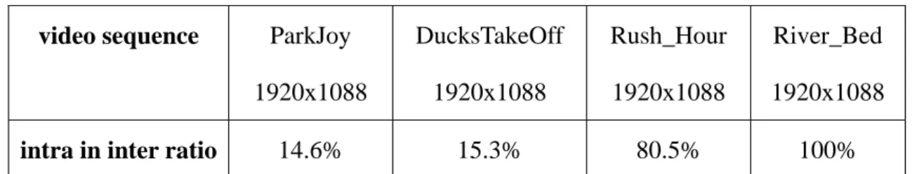
PCM modes. For example, Table 1 shows the ratio of intra macroblocks in inter-frame for some high quality video sequences, encoded by AVC/H.264 reference software JM 16.1. This ratio will be increased when the object has large motion or

complex texture, such as the MPEG HD test sequences Rush_Hour and River_Bed. Since the quality of inter-coded macroblocks also depends on these intra-coded

macroblocks, intra coding efficiency becomes a key factor for high quality video applications. Secondly, for video studio editing and archiving applications, intra-only

video coding has always been a preference since it facilitates non-linear editing and causes less image processing and editing distortions than complex inter-frame video

coding techniques. Thirdly, transfer of uncompressed raw video data across hardware system buses or transmission cables is becoming expensive as the video resolution increases towards ultra-HD (8K4K) format. Traditional practices to solve this problem is to apply chroma-channel sub-sampling (e.g. YCBCR 4:2:0) or interlacing

sub-sampling. However, these sub-sampling techniques are not acceptable for super high quality video sequences. To fulfill this application requirement, some technical

requirement proposal has been submitted to ISO/IEC MPEG organization to request for a new standard for a low-complexity, fixed rate intra-only video coding standard

2 [32].

video sequence ParkJoy

1920x1088 DucksTakeOff 1920x1088 Rush_Hour 1920x1088 River_Bed 1920x1088

intra in inter ratio 14.6% 15.3% 80.5% 100%

Table 1 ratio of intra blocks in inter-frame (average video quality at 44dB)

Although spatial prediction tool in AVC/H.264 increases efficiency of intra coding significantly, it does not work well for macroblocks with complex textures.

In this thesis, we try to design a new intra codec that adopts a new mathematical model for prediction with the following characteristics:

 The coding process requires very little coding buffer. For some of the

near-lossless applications mentioned above, coding buffer is an expensive

resource. For example, for near lossless video transport across system buses and cables, it would be too expensive to include large coding buffer on the

sender-side and the receiver-side. Preferably, there is an option to perform scanline-based linear coding/decoding without any buffer.

 The codec complexity is low and the operations can be parallelized without

much efficiency loss. Sequential coding algorithms may access more

reconstructed information to achieve higher prediction accuracy, it cannot be parallelized. For applications that requires high coding throughput, this

may be an issue.

 The codec is targeted for very high quality video applications. With the

development of new generations of display systems, high quality video content is becoming more and more important. As shown in Table 1, when

video quality reaches 44dB (or above), intra coding becomes more important. For low bitrate applications, one cannot allocate too many bits to

3 design philosophy may change and allows for more overhead in predictor

description to reduce overall coding distortion.

 Fixed compression ratio can be achieved without complex rate control

algorithms. Again, some applications require strict constant bitrate of the compressed content (i.e. fixed compression ratio throughout the whole

sequence). However, with traditional video compression techniques fixed compression ratio is very hard to accomplish with single-pass rate control

algorithm, if possible. However, multi-pass rate control algorithm requires large coding buffer and high complexity. This makes it very difficult to

design in-circuit real-time compressor and decompressor. With fixed compression ratio, video data can be transmitted in fixed clock cycles and

transmission delay can also be controlled precisely, which is ideal for near-lossless raw video transmission over system buses or cables.

The organization of the thesis is as follows. Chapter 2 conducts a survey on existing image coding techniques and presents the design of two most popular intra

coding standards, namely the JPEG image codec and the AVC/H.264 intra codec. Chapter 3 presents the framework of the proposed one-dimensional intra codec with

excitation-based prediction. The coding of residual signals is discussed in Chapter 4. Integration of the proposed image codec into H.264 video codec is described in

Chapter 5 and some experimental results are given in Chapter 6. Finally, some conclusions and discussions are given in Chapter 7.

4

Chapter 2. Previous Work

In section2.1, many image coding methods are briefly described. The popular

still image coding standard (JPEG and JPEG2000) are illustrated in section 2.2. AVC/H.264 intra codec is also introduced. Due to advanced spatial prediction tool,

AVC/H.264 intra codec outperforms both JPEG and JPEG 2000 for general image coding. In section 2.3, some speech codecs are presented.

2.1. Overview of image coding

There are many different image coding algorithms. Different transform coding methods are developed, such as discrete cosine transform and wavelet transform. In

[1], they introduce a new approach to image compression based on decomposing the image using the orthogonal wavelet transform. From the analysis of these transform

codecs, wavelet transform outperforms 1dB than DCT in still image coding, but it is less obvious for video coding [2]. Instead of scalar quantization, vector quantization is

also introduced to image coding [3]. To judge the performance of coded image quality, an objective quality measurement is also an important topic. Peak

signal-to-noise ratio (PSNR) is a common measure of video quality. Structure similarity index (SSIM) is an image quality measure which has been shown to be

more consistent with human perception for medium quality contents [4].

Some image and video coding standards will be discussed in the following

sections.

2.2. Design examples of image coding standard

In this chapter, I will introduce the still image coding method which is popular in

5 algorithm is presented in section 2.2.1. In section 2.2.2, I will briefly describe H.264

which has higher coding efficiency in video compression technology. And the video processing flowchart is also detailed in this section.

2.2.1. JPEG image coder

For the past few years, a joint ISO/CCITT committee known as JPEG (Joint Photographic Experts Group) has been working to establish the first international

compression standard for continuous-tone still images. JPEG features a DCT-based

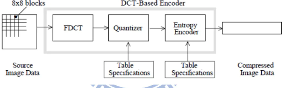
lossy compression and it is sufficient for a large number of applications. In Fig. 1, we could clearly see that coder includes three main parts: transform, quantization, and entropy coding. The image is processed block by block.

Fig. 1 DCT-based encoder processing steps

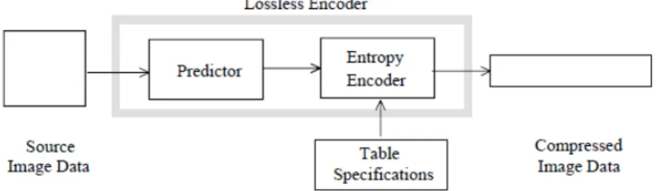
JPEG also supports lossless compression using prediction method, which is

called JPEG-LS, and this encoder structure is shown in the Fig. 2. JPEG-LS is a late addition to the JPEG standard. Encoder can access the left, upper-left, upper blocks as references to predict the current block. Lossless codec typically produce around 2:1

compression for color images with moderately complex scenes [5]. More information can be referenced in [6].

6

Fig. 2 lossless mode encoder processing steps

While JPEG2000 provides an advantage in compression efficiency over JPEG,

its primary advantage lies in its rich feature set. Central to this standard is the scalability that allowing image components can be accessed at different resolution and

spatial region of interest [7]. Two primary reasons for JPEG2000’s superior performance are the wavelet transform and embedded block coding with optimal

truncation (EBCOT) [8].

2.2.2. H.264 intra coder

The major video coding standard like MPEG-2, MPEG-4 Visual, and H.264

incorporates motion estimation (ME) and compensation (MC), a transform stage and entropy coding. The model is often described as hybrid DPCM/DCT codec [9][10].

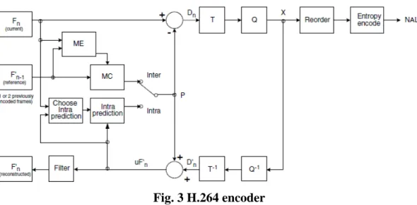
H.264 is the most high performance video codec in today, Fig. 3 shows H.264 encoder flowchart. The encoder includes two dataflow paths, ‘forward’ path is from

left to right and ‘backward’ path is from right to left. Because encoder side needs the reconstructed image to predict next frame, backward path is the reconstruction path

7

Fig. 3 H.264 encoder

H.264 also processes the images in blocks and can divide the image into more

small blocks compared to JPEG. H.264 contains three prediction modes: intra prediction, inter prediction and bi-directional prediction [11]. Intra prediction exploits

spatial correlation within one picture. In intra prediction (I-frame), the neighboring reconstructed macroblocks in current frame are used to predict the current macroblock.

If the I-frame is also an IDR-frame, the latter inter-frames cannot access the previous frame before IDR-frame as reference frame. This IDR-frame is designed for random

access in the video. For inter prediction (P-frame), previous reconstructed images are used to predict the current frame. This part involves motion estimation and motion

compensation, and encoder can select the best reference frame joint rate and distortion optimization. Macroblocks in inter-frame also can be coded in intra blocks. When

there is a scene change, many macroblocks will be coded in intra blocks. And H.264 also provides bi-directional prediction (B-frame), encoder can reference more

reconstructed frames to improve the prediction accuracy.

After prediction using different modes, the prediction error, residual frame, is

transformed to another domain for removing the correlation. H.264 uses integer discrete cosine transform (DCT) for reducing the multiplication operation which can

8 coefficients include two parts, AC coefficient and DC coefficient. DC is the measure

of average value of image samples. There is strong correlation between DC coefficients of blocks so Hadamard transform is further used to compact the data

energy again. Current two-dimension transform includes two sizes, 4x4 and 8x8. After the transformation, data is quantized according to different quantization step size.

H.264 also supports rate-control which can adjust the quantization step dynamically at frame level and macroblock level to approximate the required bitrate.

The entropy coding in H.264 contains two methods, context adaptive variable length coding (CAVLC) and context-based adaptive binary arithmetic coding

(CABAC) [12]. Huffman coding needs to calculate the probability of each symbol and assign the integer bits for each symbol. But there are two disadvantages, we need

to transmit the probability tables and it also cause time delay. So CAVLC uses the fixed code-table which is trained by various video materials to encode the symbol and

the previous information is referenced in the encoding process. On the other hand, arithmetic coding transmits the whole symbols as a codeword, so it can be more close

to the optimal bitrate compare to Huffman coding. It’s obvious that using integer number of bits for each symbol is unlikely to come so close to the optimal number of

bits. Therefore the arithmetic coding can outperform the Huffman coding. H.264 also contains many context probability models to model the feature of data and the

probability model is converged in the encoding process. This design improves the coding efficiency and cause CABAC to outperform CAVLC.

Compare to JPEG and JPEG2000, still image coding in H.264 has higher coding efficiency because it involved the enhanced intra prediction algorithm and the

deblocking filter. In [13][14], they investigate the performance of H.264 intra coder and compare the quality of image, and the complexity with the commonly used image

9 has better performance than JPEG and JPEG2000. H.264 intra coding and JPEG2000

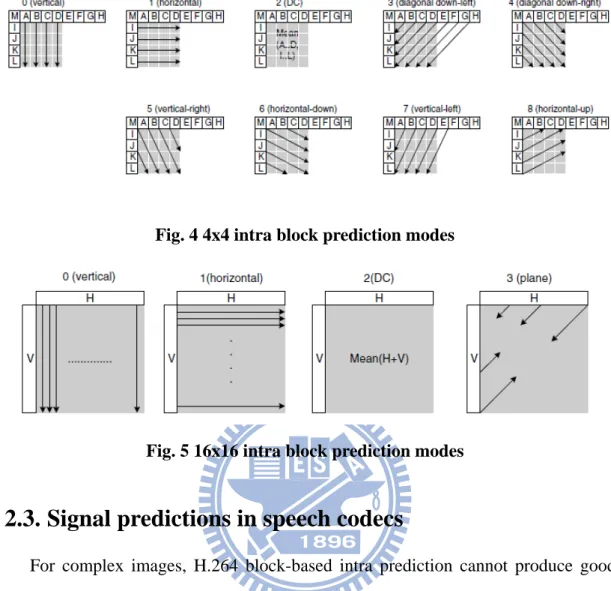
has similar performance at low bitrate condition, such as 1 bit per pixel. H.264 has 4 different prediction directions for 16x16 MBs and 9 different prediction directions for

4x4 blocks [15] shown in Fig. 4 and Fig. 5. Few approaches are proposed to reduce

the complexity of intra coding. In [16], they limit the intra prediction modes using the

directional information at the 16x16 prediction mode. In [17], early termination is decided by the computation of cost function and selective computation of highly

probable modes. And the paper [18] presents a three steps algorithm for H.264 4x4 intra prediction.

H.264 spends little bits at prediction so the prediction quality is worse at the complex areas. There are also some papers proposed to improve intra-frame quality.

In [19], they consider the distinct image singularities within the model of piece-wise smooth functions, etc edge. In [20],template matching is introduced to the subset of

current predictor set. It’s useful when the image contains repeated patterns but it suffers the problem of parallel encoding. Line-based and resample-based intra

prediction is also proposed in [21]. Resample-based intra coding is suitable for the high definition videos. However, intra prediction quality is still worse on complex

contents and it doesn’t remove the coherence between signals. That results in high residual bitrate at entropy coding stage. If we can find the trade-off between

prediction header cost and residual bitrate, the overall codec performance will be improved.

10

Fig. 4 4x4 intra block prediction modes

Fig. 5 16x16 intra block prediction modes

2.3. Signal predictions in speech codecs

For complex images, H.264 block-based intra prediction cannot produce good

predictor. Its method is suitable for smooth area but not for highly textured area, like grass and waves in the image. One way to handle prediction of complex signals with

repeated patterns is to use the coding method similar to speech coding to capture the edge information and the texture information of the image [22]. We can describe the

texture of the image using a way similar to speech codec to depict the formant of the voice without the constraint of the block shape. Images can be converted to

one-dimension information and then processed in one dimension domain.

Speech codec process the signals using linear prediction filter first, and then

prediction error called excitation is down-sampled by closed-loop or open-loop method. The number of reserved excitation represents the bitrate directly. Excitation

11 RPE-LTP based codec not only reserved the excitations by open-loop method but also

apply long-term prediction to catch the peak period of the voice [23]. In the previous experiments, it is shown that we only need to reserve 1/3 excitations and can simulate

the speech well enough. Some speech codec also use excitation code-book to select the proper excitations, and reduce the bits allocation for recording excitation with the

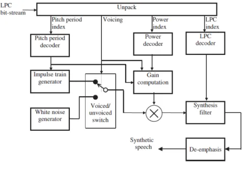
transmission of the code-book index. CELP-based method is one of the cases. Fig. 6 is the simple diagram of the LPC decoder. From the figure we can clearly see that

impulse train generator is for simulating the pitch period, and gain computation is mainly related to the energy level of the signal, and synthesis filter specify the

synthesis coefficients for reconstructing signals.

Fig. 6 LPC-based speech decoder

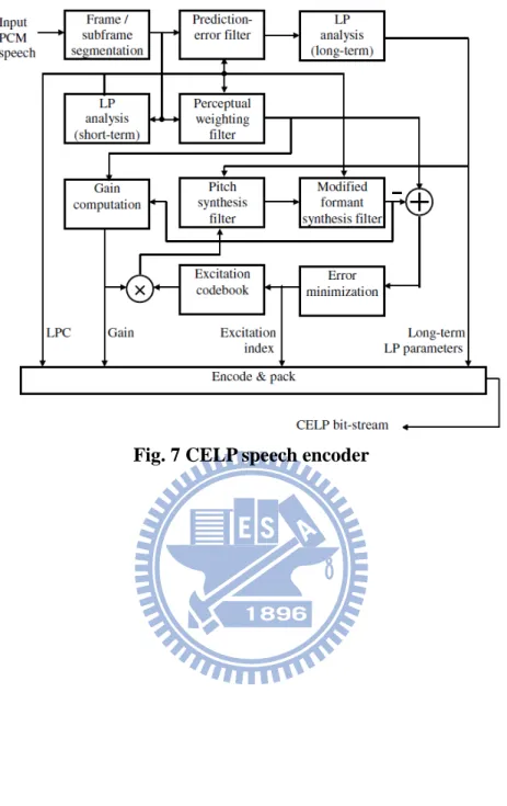
Fig. 7 shows the block diagram of a generic CELP encoder. The perceptual weighting filter in the diagram is for adjusting the prediction errors because human is sensitive to specific frequency band. So prediction error in different frequency band

may have different weighting. Excitation code-book is trained by the input signals, and this design is also a “close-loop” CELP encoder because it involves the error

12

13

Chapter 3. Proposed Intra Coding Method

Because we want to remove the artifacts of block-based prediction and predict

the repeated complex pattern more correctly, we try to predict the signals in one-dimensional domain with more flexible algorithms. Two-dimensional image

blocks will be scanned into one dimension data using Hilbert’s scanning order [24]. For the investigation in this thesis, 1616 macroblock size is scanned into 1-D signals using pre-computed Hilbert scan path. After expanding the 2-D image to 1-D 256 signals, different prediction methods will be applied according to the feature of the

signals. The signals are classified in two categories: smooth signal and textured signal. Fixed segment length is proposed in current coding structure and each segment

contains 16 samples. It can be observed that each pixel has close relation with neighboring pixels so the Hilbert scan path is able to convert a 2-D signal to 1-D

while maintain the spatial similarity within image pixels. A brief summary of the proposed intra-coding mechanism is described as follows.

For textured segment, we model the prediction error as random noise. First step, Signal is analyzed by order one linear prediction filter after segmentation. And then

prediction error is down-sampled using closed-loop (analysis-by-synthesis) method. The excitations are down-sampled irregularly with minimal spatial errors. For this

purpose, the synthesizer is also included at the encoder side to minimize prediction errors in spatial domain. Original magnitude of the excitation is modified at the

synthesizer for better prediction. Instead of uniform scalar quantization, vector quantization is used at the predictor description for textured segment to decrease the

header bitrate. Arithmetic entropy coding is also applied to the predictor syntax. Some context model is also designed for different header syntax to approximate optimal

14 bitrate. For smooth segment, we simply compute the mean of the samples and apply

uniform scalar quantization for prediction. The details of each step of the proposed algorithm are presented in the following sections.

3.1. Intra Prediction Block Diagram

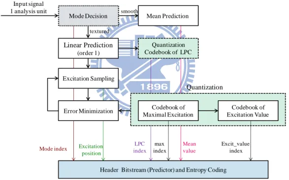
Fig. 8shows the proposed intra prediction framework and the syntax of predictor description. The mode decision module segment the input signal unit into smooth unit

or textured unit. For textured unit, the predictive coder is composed of three main parts: LP filter, excitation sampling, and quantization. After the predictive coder, the

predictor parameters are quantized and entropy coded.

Fig. 8 proposed intra prediction structure

3.2. Preprocessing

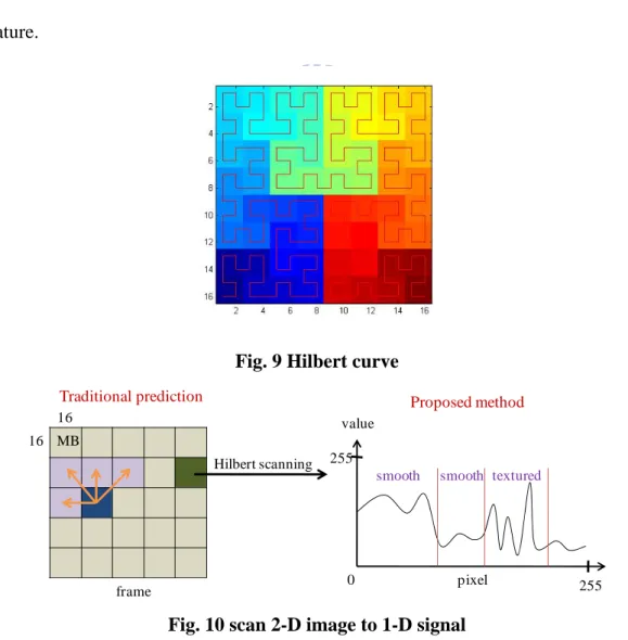
3.2.1. Hilbert scanning

The Hilbert curve is a space filling curve that visits every point in a square grid

and it was described by David Hilbert in 1982. Hilbert curve has been widely used in image processing because the coherence in neighboring pixels is very important. It is

also widely believed that Hilbert-space filling curve can achieve best clustering

Mode Decision Linear Prediction (order 1) Input signal 1 analysis unit Excitation Sampling Codebook of Excitation Value Codebook of Maximal Excitation Quantization Codebook of LPC Mean Prediction Error Minimization

Header Bitstream (Predictor) and Entropy Coding

Quantization

Mode index Excitation

position LPC index max index Mean value Excit_value index smooth textured

15 [24][25][26]. We can produce Hilbert curve in different resolution recursively and

apply to 2n x 2n image. 2-D image is scanned into 1-D signals using Hilbert’s

method, as shown in Fig. 9. Curve starts from left-bottom corner and ends at right-bottom corner. Hilbert’s method reserves the signal similarity so this pattern is used to process the signals in one dimension. Because we may integrate our intra

prediction method with current prediction methods in H.264, 16x16 block size is proper for scanning. This helps the further integration by intra mode decision at

macroblock level. And each macroblock in the frame is preprocessed like the Fig. 10 from upper-left to bottom-right. 1-D signal is further processed according to their

feature.

Fig. 9 Hilbert curve

Fig. 10 scan 2-D image to 1-D signal

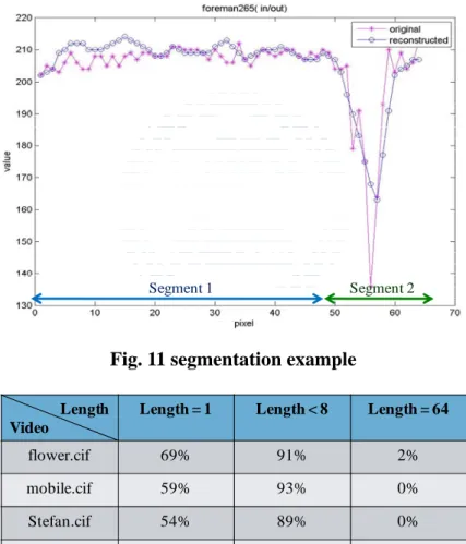
3.2.2. Segmentation

Signal is classified by three factors: variance, average value, and the intensity

16 16 MB Hilbert scanning 0 pixel ₂₅₅ value 255

Traditional prediction _{Proposed method}

smooth smooth textured

16 difference between neighboring pixels before we apply different algorithms to encode

the signals. Signals have same features will be merged and the length of segment is

adaptive. Fig. 11 is the example of segmentation, and the segment 1 is processed as smooth segment, and the segment 2 is processed as textured segment. From the

experiments of 4 cif sequences, Table 2, there are average 64% segments which length is equal to one analysis unit (16 samples). On the other hand, more bits is allocated for recording segment length, so fixed segment length (1 analysis unit) is

used at current design structure.

Fig. 11 segmentation example

Table 2 segment length

3.2.3. Increase bit depth of signal

To get higher prediction accuracy, the signals bit depth is extended from 8 bits to

11 bits. This way can decrease the rounding effect in the encoding process. And the

Segment 1 Segment 2

Length Video

Length = 1 Length < 8 Length = 64

flower.cif 69% 91% 2%

mobile.cif 59% 93% 0%

Stefan.cif 54% 89% 0%

foreman.cif 77% 100% 0%

17 post processing function is also needed to rescale the signal.

3.3. Mode decision

After scanning the 2-D signal into 1-D signal, different prediction method is used according to the feature of the signals. The variance of the signal is the mainly

measurement for its characteristic. In my proposed method, segment length is fixed in 16 samples at current stage. So we don’t need to spend more bits of recording the

segment length. Segment mode is decided by the fixed threshold. If the signal is smooth, I use simple mean value of the segment to predict. Otherwise, if the segment

has variance larger than the threshold, more flexible algorithm is applied to achieve better prediction quality. Fixed segment length could decrease the bits for segment

length description but neighboring segment may have similar feature. We may need to combine the segments which have same feature in the future. Two prediction modes

are supported in current intra prediction structure and spend one bit of storage.

3.4. Linear prediction (Analyzer)

If the segment is textured, we used more complex prediction algorithm. First, I

assume the signal x[n] is regressed on previous values of itself, plus an error term v[n]. And the a1, a2,…, aM are known as the autoregressive (AR) parameters and the v[n]

represents a white noise process if the prediction order is higher enough.

x n a x n 1 a x n 2 ⋯ a x n M v n

x n a x n 1 ⋯ a x n M v n

HA(z) denotes the system function of the AR analyzer and the direct form

realization is shown in the Fig. 12. This filter takes x[n] as its input and v[n] as its output. This all-zero filter (FIR) transforms an AR process at its input and white noise at its output.

18

H z V z

X z   a z

Fig. 12 direct form realization of analyzer

From the experiment result, order 3 filter can achieve good prediction quality.

When prediction order is higher than 3, it’s nearly useless. The relation between luma

residual bitrate and the order of LP filter is shown in Fig. 13. It is obvious that LPC order converges at 3 coefficients because textured segment has lower correlation between neighboring signals. But in the actual implementation, the bits allocation of

LP coefficients and the resulting residual bitrate are both considered. I select order 1 filter in my proposed prediction structure.

Fig. 13 comparison between luma residual bitrate and LPC order

3.5. Synthesizer

Decoder includes the synthesizer to reconstruct the signals. Encoder side also needs the synthesizer for optimal excitation down-sampling. Various excitation

positions are selected and reconstructed excitations are the input of the synthesizer at ] [n v ] [n x a1 aM 1 aM

z

z

z

19 encoder side. So encoder can simulate the operation of decoder side, and find the best

position of excitation by minimizing the spatial domain errors. Because encoder selects the excitation through synthesizer, this method is called “analysis by synthesis”

or “close-loop” method. On the other hand, excitation also would be quantized for transmission, so we can more accurate simulate the decoder’s operation by including

the quantization process in close-loop method. And the optimal excitation value is found by the synthesizer by reconstructing the original signal value. Although this

design would be more complex and time consuming compared to open-loop method which doesn’t include synthesizer at encoder, we can increase the prediction precision

and hence decrease the residual bitrate in latter part.

Synthesizer is an IIR filter to synthesize the signals by filtering white noise using

all-pole filter. Synthesizer filter and the direct form realization are illustrated in Fig.

14. There is an order 1 synthesizer corresponding to the order 1 analyzer at encoder

side. H z X z V z   1 H z   1 ∑ a z

Fig. 14 direct form realization of synthesizer

3.6. Excitation sampling

After signal is processed by LP filter, excitation should be down-sampled for

storage and transmission. The textured segment is more difficult to predict so has higher excitation amplitude, we should reserve more excitations to catch the valley or

] [n v x[n] a  1 aM  1 aM 

z

z

z

20 peak which may be the edge or texture in the image. 5 excitations are reserved in each

segment (nearly down-sample 3). And the position of excitation is selected by minimization the difference of original signal value and the reconstructed value. This

part includes the synthesizer for reconstructing the original signals and quantization error is also in consideration.

Example in Fig. 15 shows the residual distribution in frequency domain, and it’s clearly that RPE-based method has lower residual energy compared to H.264 intra

coding. Using fixed grid excitation selection and open-loop method to find the fine excitation positions is simple but not optimal. Open-loop method only considers the

total error magnitude after the excitation selection. It doesn’t reconstruct the signals and compare the prediction error in spatial domain. Thus I use closed-loop method to

choose the excitation optimally and adjust the excitation amplitude when synthesizing the signals. Adjust the original value of excitation can construct more accurate

reconstructed value by the synthesizer at decoder side. Optimal excitation amplitude can be reconstructed through synthesizing at encoder. The simple system diagram of

closed-loop method is shown in Fig. 16. In Fig. 17, the residual distribution is shown before and after we modified the excitation value properly. It reveals that the error

distribution using our proposed method is scattered in frequency domain and the residual energy is much lower. After excitation sampling in the below diagram,

quantization process is applied to excitations in my implementation. Thus the synthesis filter can get the same information as decoder side.

21

Fig. 15 residual distribution of H.264 intra coding and RPE-based method

Fig. 16 closed-loop encoder (analysis by synthesis)

Fig. 17 residual distribution of irregular excitation selection and modified the excitation value properly

0 1 2 3 4 5 6 7 8 9 10 11 12 13 14 15 0 50 100 150 200 250

MB191 after transformation (block1)

frequency ma g n it u d e H264 RPE-based LP analysis Synthesis filter Error minimization Excitation sampling Encode and bitstream Input signal LPC Excitation position and amplitude 0 1 2 3 4 5 6 7 8 9 10 11 12 13 14 15 0 10 20 30 40 50 60 70

MB148 after transformation (block1)

frequency ma g n it u d e IrrExcit IrrExcit+Modified

22

3.7. Quantization

The description syntax of the predictor is also quantized to reduce the header

bitrate. This part contains the quantization of linear prediction coefficient and excitation value for textured segment. In smooth segment, we only use uniform scalar

quantization on the average value of the signals.

For the textured segment, excitation is further divided to two parts: magnitude

of maximal excitation and the ratio of excitation value relative to maximal excitation value. It means each segment contains one maximal excitation magnitude and 5’s

relative rations. It is well know that vector quantization has better performance than scalar quantization. So instead of scalar quantization, vector quantization is used in

coding the excitation ratios and the vector code-book is trained by different video materials. Code-book is fixed in the codec so we don’t need to transmit it. And

Code-book size will be discussed in following sections.

3.7.1. Linear prediction coefficient

Linear prediction coefficient is converted to reflection coefficient (RFC) first.

Because using the reflection coefficients allows a straightforward supervision of

stability status, since the condition RFC 1 can easily be monitored. RFCs also can be found from the lattice filter structure, in Fig. 18 [22]. Four different video materials and 1/3 frames of the videos are selected for training the vector quantization

code-book of RFC. Smooth video like foreman.cif and the more complex video like flower.cif are included. Due to the trade-off between header bitrate allocation and

23

Fig. 18 implementation of lattice structure of all-pole filter (top) and all-zero filter (bottom)

3.7.2. Maximal excitation

After we down-sampled the excitations using close-loop method, maximal

excitation is sampled in these excitations and a quantization code-book is trained for its magnitude. From the experiment result, proper code-book size is 32 and it’s

sufficient to represent the amplitude. To signal the 5 excitations values, I only need to record the amplitude ratio relative to the value of maximal excitation. This is called

adaptive quantization (ADPCM). This design can encode the excitation amplitude in more flexible way.

3.7.3. Excitation value

As discussed previously, the amplitude of the reserved excitations is recorded as the ratio relative to the value of maximal excitation. For this part, I apply vector

quantization instead of scalar quantization to approximate the optimal bitrate. The code-book size may be limited by available memory, so the proper code-book size is

256x5 by experiments. Each segment has 5 ratios and code-book contains 256 vectors.

For simulating the operation at decoder side, encoder side will run 256 times to find the best quantization vector and the quantization error is computed at the

24 synthesizer. Although it has higher time and computation complexity at the encoder

side due to optimal quantization code-book selection but it still not affect the complexity of decoder side and improve the prediction accuracy.

3.8. Predictor entropy coding

The description of the predictor should be further coded for transmission and storage. Arithmetic coding is used for entropy coding. Like the CABAC in H.264, a

context model is constructed for encoding segment mode assuming the neighboring segments may have similar feature. And 16 context models are designed to encode the

position of excitations. For the other predictor syntax elements, I simply use equal probability to encode the symbols. H.264 uses probability table to update the context

probability and prevents the multiplication operations. Because my proposal is integrated into JM16.1 directly, transition rule and transition table of probability in

JM16.1 is reused for my intra predictor.

3.8.1. Segmentation mode

Each segment cost one bit for recording segmentation mode, smooth or textured.

Because the neighboring segments may have similar feature, I design a context model for syntax probability distribution. And from the experiments, this can save nearly

30% bits.

3.8.2. Excitation position

There are 16 samples in a segment and 5 positions of reserved excitations are

recorded. If we encode the position directly, we will spend 20 bits of each segment. So some context models are designed for recording the position of excitation in a way

similar to the encoding of significant map in H.264. In the binarization process, every position has a corresponding context model. If excitation is reserved in this position,

25 using arithmetic coding. And from the experiment result, it shows that this method

can save nearly 30% bits. Binarization rule is illustrated in Fig. 19, and the symbol is coded from first position to the last position. Because we already know the excitation

count is 5, we don’t need to encode the last excitation (marked X in the figure) in this example.

Fig. 19 binarization of excitation position

0 20 0 0 0 0 30 0 -6 0 0 0 0 17 2 0

0 1 0 0 0 0 1 0 1 0 0 0 0 1 1 X

Excitation value Binary map

26

Chapter 4. Proposed Residual Coding

The residual in each image block is transformed, quantized, and entropy coded into the compressed bitstream. In this chapter, we discuss the details on transform

coding and entropy coding.

4.1. Transform coding

Because the proposed intra prediction method processing signals in

one-dimension domain, the original 2-DCT in H.264 should be removed and redesign a suitable 1-D transform. On the other hand, the quantization process in H.264 is

integrated with transformation for decreasing rounding errors and H.264 also support adaptive quantization which models the distribution of quantization error, so the

quantization process is also redesigned for my proposed method. We will discuss these processes from this section.

Spatial domain information can be transformed to another domain and data in transform domain should be de-correlated and compact. I apply 1-D integer cosine

transform (ICT) on residual information using the theory of dyadic symmetry [27].

Definition of dyadic symmetry: A vector of 2m elements a , a , ⋯ a is said to have the ith dyadic symmetry if and only if a s ∙ a_⨁ , where ⊕ is the “exclusive or” operation, j ∈ 0, 2 1 , and i ∈ 1, 2 1 . s = 1 when the

symmetry is even and s = -1 when symmetry is odd. Detail theory of dyadic symmetry can be referenced at [28][29]. We can use this property to convert DCT to

ICT.

To eliminate the floating point arithmetic so the real magnitudes of the DCT

component is approximated by 8-bit integers. The paper [27] shows how to convert the order-8 cosine transform into a family of integer cosine transform. And an

27 order-2n T i, j orthogonal transform can be generated from an order-n T i, j transform as follows:

(a) The first n basis vector of T i, j : T i, j = T i, j

And T i, 2j 1   T   i, j     for  j ∈ 0, n 1 (b) The last n basis vectors of T i, j :

(i) T i n, 2j   T   i, j  

And T i n, 2j 1   T   i, j     for  j ∈ 0, 2,4, … , n 2

(ii) T i n, 2j   T   i, j   

And T i n, 2j 1   T   i, j     for  j ∈ 1,3,5, … , n 1

The above generation rules are used to compute the order-16 ICT coefficients and then transform matrix is applied to residual frame.

4.2. Entropy coding in H.264

There are two different entropy coding methods in H.264: context adaptive variable-length coding (CAVLC), context adaptive based arithmetic coding (CABAC).

In this chapter I will introduce these methods briefly and then discuss the drawback of current design. I also proposed a modification of CABAC which can reduce average

7% bitrate for very high bitrate videos. Proposed modification in CABAC is introduced in the last section.

4.2.1. CAVLC

Before the variable length coding, H.264 uses zigzag scan on the block to get the

transform data from low frequency to high frequency. Zigzag scan is shown in the Fig.

20. Run-length coding is applied to the scanned information. The number of continues

28 catch the distribution of the signals, various VLC tables are selected according to the

run-length codes. The transition rule between different VLC tables is also identified in the current H.264 codec. Because most coefficients in high frequency band are zeros,

VLC table will assign fewer bits for continuous zeros and small magnitude of high frequency coefficients. The VLC table is trained by various video sequences and its

mapping characteristic is for the signal which contains large energy at low frequency band.

Fig. 20 zigzag scan

4.2.2. CABAC

Arithmetic coding can achieve better coding efficiency compared to variable length coding because it represents the series data in one long floating number and

approach the optimal fractional number of bits required to represent each symbol. This prevents the integer bits assignment of each symbol, like Huffman coding. The

idea of arithmetic coding is illustrated in the Fig. 21. For example, there are two symbols, A and B. We already know the probability of A is 0.3 and probability of B is

0.7. When we read the symbol B, we can use the floating number in [0.3, 1] to represent B. After reading the second symbol B, [0.51, 1] represents “BB”. Finally,

the floating number in [0.51, 0.657] represents “BBA”.

H.264 prevents the multiplication operation on floating number, so a 9 bits

integer variable is used for representing the floating number in H.264 and H.264 outputs the codeword by shifting the variable.

29

Fig. 21 example of arithmetic coding

H.264 not only designs different context probability models for different syntax

but also has many probability models for each syntax element. Each syntax element has its own data distribution, so it should be model by a specific context probability

model. First, the context model is initialed for different syntax according to different frame type and quantization scale, and these models will be adjusted by different

video contents. H.264 will binaries the symbol first, and then put it to arithmetic entropy coder. By combining an adaptive binary arithmetic coding technique with

context modeling, a high degree of adaptation and redundancy reduction is achieved.

CABAC coding flowchart is shown in Fig. 22[12]. We can better approach the entropy bitrate of the signals by this process. To decrease the complexity of multiplication operation, H.264 use fixed probability transition tables to update the

context model. Probability quantization is also involved in the transition table for the limited memory.

P(A)=0.3 P(B)=0.7 Encode BBA in [0.51,0.657] 0 1 0.3 1 0.51 1 0.51 0.657 0.3 A B B B A

30

Fig. 22 CABAC encoder block diagram

4.2.3. Issues of CAVLC/CABAC in H.264

Current intra/inter prediction in H.264 is not sufficient so the residual

information still contains much similarity. For example, motion estimation is bad if the object has large motion. When the video content is too complex, intra block is

needed in inter frame. Moreover, more blocks will be coded in PCM mode. In the transform domain, most blocks energy is compacted to low frequency band. Current

entropy coding structure of CAVLC/CABAC is still designed for the data which contains much energy at low frequency band and lower energy at high frequency band.

If the block contains higher energy in high frequency band or the energy is scattering, we may spend more bits in entropy coding because the current model is not suitable

for these features.

Run-length coding in CALVC scans the number of continues zeros and the

magnitude of non-zero coefficient. Run-length code is encoded from low frequency to high frequency band. Transition between different VLC tables is decided by the

threshold which is fixed in each VLC table. Current threshold of the high frequency band is smaller compared to the other bands. If residual data have larger amplitude at

this band, VLC table will assign many bits to encode the coefficient. This would be a drawback of current CAVLAC model. In [30], they redesign a VLC-table for lossless

31 saving compared to the original CAVLC scheme in H.264.

CABAC has divided the transformed coefficient coding into two parts, significant map and significant coefficient. Significant map is for recoding the

position of non-zero coefficients and significant coefficient is for the coding of non-zero coefficient value. CABAC also further split the significant coefficient into

two parts, absolute part and one part. Value one is coded first and the remaining magnitude is further coded at absolute part. Most entropy bitrate comes from the

magnitude of transformed coefficients. CABAC in H.264 designs 5 context models to capture the data distribution and the transition between different context models

depending on the magnitude of the coefficients. If energy is scattering, this design is not suitable. On the other hand, significant map will allocate more bits when energy is

scattering because context model cannot predict the position of non-zero coefficient. Although CABAC has 16 context models for significant map, it’s still not proper

when energy is scattering or under large quantization scale condition.

4.3. Proposed modification in CABAC

CABAC has higher bitrate than CAVLC where their reconstructed video quality

is almost same under high bitrate condition. Five HD video sequences are tested and

the result is shown in Table 3. From the experiments, I found that there is a problem in the encoding of significant coefficient. CABAC encoding the magnitude of coefficient uses fixed threshold (value is 13) to divide the magnitude to two parts. If

coefficient magnitude is smaller or equal to this threshold, CABAC will encode the magnitude use many context probability models. And the probability model will be

updated through encoding process. Otherwise, CABAC encode the magnitude with equal probability model.

32

Table 3 bitrate comparison of CAVLC and CABAC

However, for the lossless or high bitrate videos, coefficient magnate will be large,

so the threshold should be smaller. Moreover, this threshold should be adjusted according to different bitrate or quantization scale. To measure the effect of adjusting

threshold, the original threshold in CABAC is modified and found that if we could adjust the threshold dynamically in different quantization scale, we can have more

bitrate saving under high bitrate or lossless condition. Experiment result using 4 CIF

sequences is shown in the Fig. 23toFig. 25. It reveals that this adjustment can lead to

average 7% bitrate saving for nearly lossless compression.

Fig. 23 flower.cif bitrate saving video method flower (48dB) mobile (47.6dB) stefan (51dB) city (50.8dB) funfair (50.7dB) CAVLC 14587 14560 13128 11877 14497 CABAC 15780 14893 13725 11800 14402 Kbit/s 25400 25600 25800 26000 26200 26400 26600 26800 27000 3 5 7 9 11 13 15 17 19 21 kbit/s threshold qp4 qp4 0 5000 10000 15000 20000 25000 3 5 7 9 11 13 15 17 19 21 kbit/s threshold qp12 qp12 12200 12250 12300 12350 12400 12450 12500 3 5 7 9 11 13 15 17 19 21 kbit/s threshold qp20 qp20 9710 9720 9730 9740 9750 9760 9770 9780 9790 9800 9810 3 5 7 9 11 13 15 17 19 21 kbit/s threshold qp24 qp24 gain: 1% gain: 13% gain: 0.5% _useless

33

Fig. 24 mobile.cif bitrate saving

Fig. 25 foreman.cif bitrate saving 15000 18000 21000 24000 27000 30000 33000 36000 39000 3 5 7 9 11 13 15 17 19 21 kbit/s threshold qp4 qp4 17500 18000 18500 19000 19500 20000 20500 21000 21500 22000 22500 3 5 7 9 11 13 15 17 19 21 kbit/s threshold qp12 qp12 12200 12250 12300 12350 12400 12450 12500 3 5 7 9 11 13 15 17 19 21 kbit/s threshold qp20 qp20 9480 9490 9500 9510 9520 9530 9540 9550 9560 9570 9580 3 5 7 9 11 13 15 17 19 21 kbit/s threshold qp24 qp24 gain: 15.5% _{gain: 9.9%} gain: 0.1% _useless 16500 17000 17500 18000 18500 19000 19500 20000 20500 3 5 7 9 11 13 15 17 19 21 kbit/s threshold qp4 qp4 10320 10340 10360 10380 10400 10420 10440 10460 3 5 7 9 11 13 15 17 19 21 kbit/s threshold qp12 qp12 5430 5435 5440 5445 5450 5455 3 5 7 9 11 13 15 17 19 21 kbit/s threshold qp20 qp20 3631 3632 3633 3634 3635 3636 3637 3638 3 5 7 9 11 13 15 17 19 21 kbit/s threshold qp24 qp24 gain: 6.2% useless useless useless

34

Chapter 5. Implementation

The whole proposed prediction structure has integrated into H.264 version JM16.1 using language C. I create a new slice type called MMES_I_SLICE for our

proposed intra frame and this parameter can be set in configure file. Main profile is used for the other setting. Because we only consider the luma prediction and compare

the experiment result with H.264 in current prediction structure, we bypass the chroma processing and only compare the luma residual bitrate. Our proposed method

also can be integrated with original intra prediction methods in H.264 by mode decision at macroblock level. H.264 supports adaptive rounding in quantization

process, and this method is based on adjusting the rounding offset to maintain an equal expected value for the input and output of the quantization process [31]. The

method provides up to about 1 dB of improvement in coding efficiency performance for high PSNR encoding. So H.264 can have higher reconstruction quality compared

to our proposed method. The reconstruction quality using our method is a little worse because I only use simple uniform rounding method now. On the other hand, I don’t

take rate control into consideration at this stage.

In this chapter I will briefly describe the implementation structure and the main

encoding flowchart. And then experiment results will be presented in next chapter.

5.1. Coding structure

The start point of my proposed intra-prediction is at the function:

encode_one_slice. I also integrate the new intra prediction method into original

intra-prediction modes in H.264 using mode decision. Encoder can jointly compare

35 at macroblock level.

I construct two main structures for the implementation: filter state and segment information. “Filter state” includes the lattice filter information which is mentioned in

previous chapter. “Segment information” includes the syntax of predictor description, such as segment mode, excitation ratio, and segment bitrate, etc.

Entropy coding functions (CABAC) in H.264 are reused and context probability model is also used for my proposed method. I apply arithmetic coding on the

predictor description and the residual information. Many context probability models are also designed to catch the data distribution of the syntax in intra prediction. But

for the residual coding, I don’t have large modifications. Fig. 26 shows the coding flowchart. This picture shows the main encoding function and pipeline in H.264.

Fig. 26 encoding flowchart

5.2. Prediction bitrate

Current bitrate allocation of predictor descriptions is shown in the Table 4.   encode_one_slice() mmes_IntraCoding_Start() 16 segments? start_macroblock() Save predictor mmes_intraResidualCoding() end_encode_one_macroblock()

Set coding state

write_macroblock()

end_macroblock() yes

no

Construct the predictor

Copy proposed predictor to H.264 predictor

Coding the residual of a MB

Set the prediction mode (our proposed/H.264) Check availability of

neighboring MB

Update some parameters

36 “Reducible row” means the syntax can be modified or not in the future. “Current bits”

row shows the current bits allocation for this syntax. I assign 4 bits for the smooth segment recording the quantized mean value. It’s clearly to see we allocate more bits

for textured segment and more complex algorithm is used to improve the predictor quality. Because context model is used for arithmetic entropy coding, bitrate of

segment mode and the position of excitations will be adapted. Through the encoding process, these models can describe the feature of data gradually. For the consistency, I

use equal probability model to encode the other syntax so their bitrate is same as quantization. We also can know form the table that most bits of the predictor

description coming from the excitations. Finally, if we want to integrate the new intra-prediction mode with current intra prediction modes in H.264, we will spend 1

more bit at macroblock level.

Table 4 bitrate allocation of proposed intra prediction

Header Cost

Mode Mean value

reducible no yes

Current bits adaptive 4

Smooth segment Header Cost Mode LPC (order 1) Excitation position Maximal excitation Excitation value

reducible no yes yes yes

Current bits adaptive 3 adaptive 5 8

37

Chapter 6. Experimental Results

Two 512x512 images (Lena, baboon) and four CIF sequences are tested using my proposed intra prediction (flower.cif, foreman.cif, Stefan.cif, mobile.cif). In this

chapter, I will present the comparison of predictor quality and then show the bitrate of predictor description and residual information. Section 6.1 shows the subjective

quality of intra prediction and compares our method with H.264. Section 6.2 reveals the average bits allocation of our predictor description. And the average objective

quality is also shown in this section. I also compare the performance with JPEG, and the section 6.3 shows experiment results.

6.1. Subjective predictor quality

From the figures below, it reveals that our proposed method predicts well at the textured area. The date in the calendar is more clearly and blocking artifact is

removed from the flower garden. We successfully catch the edge or pattern in the

image by optimal excitation down-sampling. Following figures from Fig. 27 to Fig.

30 show the prediction results.

Fig. 27 mobile: left figure is our proposed predictor, 23.6dB; right figure is H.264 intra predictor, 17.9dB

38

Fig. 28 flower: left figure is our proposed predictor, 23.4dB; right figure is H.264 intra predictor, 16.7dB

Fig. 29 Stefan: left figure is our proposed predictor, 25.9dB; right figure is H.264 intra predictor, 19.8dB

Fig. 30 foreman: left figure is our proposed predictor, 28.6dB; right figure is H.264 intra predictor, 27.6dB

6.2. Predictor bitrate and predictor quality

Table 5 and Table 6 shows the header cost of our proposed intra prediction method, and the predictor quality of 4 video sequences. From the Table 6, our

39 proposed method has more than 5 dB better prediction quality compared to H.264,

except foreman.cif. Our prediction method is not good enough for the smooth video content because we only using mean prediction. However, H.264 predicts the current

macroblock by accessing neighboring macroblocks as references, so H.264 can achieve higher prediction accuracy for smooth area. Current predictor structure

allocate much bits for better prediction but bits allocation cannot be adjusted according to different quantization scale. This design cause our coding performance

will be worse for low bitrate video.

Sequence mobile flower foreman Stefan

Kbits/frame 119.4 130.1 62.1 110.4

Table 5 header cost of proposed intra prediction

Sequence mobile flower foreman Stefan

Proposed 23.58 22.93 27.89 25.91

H.264 17.95 16.69 26.76 20.04

Table 6 average intra predictor quality (dB)

6.3. Performance comparisons

Four 352x288 size images and two 512x512 size images are tested by different

coding algorithms, and the below figures show the coding performance of JPEG, H.264, and our proposed method. From the experiment results, the performance of our

proposed method is similar to JPEG for video quality is lower than 40dB. Our method can outperform JPEG and H.264 intra for very high bitrate and complex video.

Because JPEG2000 is a little worse than H.264, and outperform than JPEG, we only compare three algorithms in this experiment.

The bitrate allocation of our proposed prediction method is one of the main reasons why our performance is bad. Current prediction algorithm doesn’t take rate

40 control into consideration so prediction cost is always fixed no matter how the

quantization scale changed. However, the current H.264 intra coding only uses nearly 3 KB to describe the predictor of 352x288 image. On the other hand, we can know

that this excitation-based linear prediction algorithm is suitable for the complex repeated video content. If the video content is smooth, the original design of H.264

intra-frame coding is sufficient.

Fig. 31 flower, mobile coding performance

Fig. 32 stefan, foreman coding performance

20 25 30 35 40 45 50 55 60 65 70 0 2 4 6 8 10 ps nr

bits per pixel flower jpeg proposed H.264 20 25 30 35 40 45 50 55 60 65 0 2 4 6 8 10 ps nr

bits per pixel mobile jpeg proposed H.264 30 35 40 45 50 55 60 65 0 1 2 3 4 5 6 7 ps nr

bits per pixel

stefan jpeg proposed H.264 30 35 40 45 50 55 60 65 70 0 1 2 3 4 5 6 ps nr

bits per pixel foreman

jpeg proposed H.264

41

Fig. 33 baboon, Lena coding performance

20 25 30 35 40 45 50 55 60 65 70 0 2 4 6 8 10 12 ps nr

bits per pixel baboon jpeg proposed H.264 30 35 40 45 50 55 60 65 70 0 1 2 3 4 5 6 ps nr

bits per pixel Lena

jpeg proposed H.264

42

Chapter 7. Conclusions and Future Work

From the previous experiments, excitation-based linear prediction is applicable to the complex repeated patterns compared to the block-based prediction of H.264.

The edge and texture in the images can be described with optimal excitation selection. Although the performance of our proposed method is worse under common video

bitrate, it has outperformed the H.264 for very high bitrate videos.

The entropy coder at H.264 is reused for residual coding, but the current entropy

coder is not suitable for my proposed method. So the overall performance is not better than H.264 mainly due to the entropy coding. Although my proposed intra-prediction

method has higher prediction quality than the original method in H.264, the entropy codec should be redesign to enhance the overall performance. And the current bitrate

allocation for the intra predictor still can be decreased by more efficient excitation coding method. The bits allocation of predictor also should be adapted at different

bitrate. In the future, non-linear prediction can be involved to current prediction structure.

43

References

[1] A. S. Lewis and G. Knowles, “Image Compression using 2-D Wavelet

Transform,” IEEE Trans. Image Process., vol. 1, no. 2, pp. 244-250, Apr. 1992. [2] Z. Xiong, K. Ramchandran, M. T. Orchard, and Y.Q. Zhang, “A Comparative

Study of DCT- and Wavelet-Based Image Coding,” IEEE Trans. Circuits, Syst.

Video Techn., vol. 9, pp. 692–695, Aug. 1999.

[3] I.K. Kim and R.H. Park, “Still Image Coding Based on Vector Quantization and Fractal Approximation,” IEEE Trans. Image Process., vol. 5, no. 4, pp. 589-597,

1996.

[4] Z. Wang, A.C. Bovik, H.R. Sheikh, and E.P. Simoncelli, “Image Quality

Assessment: From Error Visibility to Structural Similarity,” IEEE Trans. Image

Process., vol. 13, no. 4, pp. 600-612, Apr. 2004.

[5] G. K. Wallace, “The JPEG Still Picture Compression Standard,” Commun. ACM, vol. 34, pp. 30-44, Apr. 1991.

[6] Information technology — Lossless and near-lossless compression of

continuous-tone still images, ISO/IEC 14495–1 and ITU Rec. T.87, 1999.

[7] D. S. Taubman and M. W. Marcellin, “JPEG 2000: Standard for Interactive Imaging,” Proc. IEEE, vol. 90, no. 8, pp. 1336-1357, Aug. 2002.

[8] K. Varma, A. Bell, “JPEG2000-Choices and Tradeoffs for Encoders,” IEEE

Signal Process. Mag., no. 11, pp. 70-75, Nov. 2004.

[9] Iain E. G. Richardson, Video Codec Design, John Wiley & Sons Ltd, 2002. [10] Iain E. G. Richardson, H.264 and MPEG-4 Video Compression: Video Coding

for Next Generation Multimedia, John Wiley & Sons Ltd, 2003.

44 Video Specification (ITU-T Rec.H.264/ISO/IEC 14 496-10 AVC),” in Joint

Video Team (JVT) of ISO/IEC MPEG and ITU-T VCEG, Apr. 2005.

[12] D. Marpe, H. Schwarz, and T. Wiegand, “Context-Based Adaptive Binary

Arithmetic Coding in the H.264/AVC Video Compression Standard”, IEEE

Trans. on CSVT, vol. 13, Issue 7, pp. 620-636, Jul. 2003.

[13] A. Al, B. P. Rao, S. S. Kudva, S. Babu, D. Suman, and A. V. Rao, “Quality and Complexity Comparison of H.264 Intra Mode with JPEG2000 and JPEG,” Proc.

IEEE Int. Conf. Image Processing, vol. 1, pp. 525-528, Singapore, Oct. 2004.

[14] Boxin Shi , Lin Liu, and Chao Xu , “Comparison Between JPEG2000 and H.264

For Digital Cinema,” Proceeding of ICME, pp. 725-728, Hannover, Germany, Apr. 2008.

[15] T. Wiegand, G. J. Sullivan, G. Bjontegaard, and A. Luthra, “Overview of the H.264/AVC Video Coding Standard,” IEEE Trans. Circuits Syst. Video Technol.,

vol. 13, pp. 560–576, July 2003.

[16] J. S. Park and H. J. Song, ”Selective Intra Prediction Mode Decision for

H.264/AVC Encoders,” Transactions on Engineering, Computing and

Technology, vol. 13, pp.51-55, May 2006.

[17] B. Meng and O. C. Au, “Fast Intra-Prediction Mode Selection for 4x4 Blocks in H.264,” Proc. of IEEE Int. Conf. on Acoustics, Speech, and Signal, vol. 3, pp. III

- 389 – 92, Hong Kong, China, 2003.

[18] C. C. Cheng and T. S. Chang, “Fast Three Step Intra Prediction Algorithm for

4x4 Blocks in H.264,” IEEE Int'l Symp. on Circuits and Systems, vol. 2, pp. 1509 -1512, 2005.

[19] D. Liu, X. Sun, F. Wu, and Y.Q. Zhang, “Edge-Oriented Uniform Intra Prediction,” IEEE Trans. Image Process., vol.17, pp. 1827-1836, Oct. 2008.