以動態投射校準技術建立之穩健車牌辨識系統

全文

(1)以動態投射校準技術建立之穩健車牌辨識系統. 學生：王倉鴻. 指導教授：陳永平博士. 國立交通大學電機與控制工程學系. 摘要在過去的二十年裡，車牌辨識的技術迅速的發展而且廣泛的被應用，如：智慧型運輸系統、電子收費系統、影像執法系統、…等等。然而，在實際應用上的問題卻造成系統辨識能力的下降，諸如不穩定的光線環境、模糊的車輛影像、骯髒或不完整的車牌字元。本論文提出一個結合空間遮罩及列差分分析的車牌粹取方法來改善車牌定位的成功率，其定位成功的比率達到 98.9%。另外，亦針對切割時產生位移、削蝕或不完整的車牌字元設計了一個動態投射校準辨識方法，其平均辨識率更達到 99.3%。若能將本論文所提出的系統以低成本硬體加以實現，將來車牌辨識技術勢必成為相關應用中普遍及重要的一環。. i.

(2) Robust License Plate Recognition System Based on Dynamic Projection Warping Technology. Student: Tsang-Hong Wang. Advisor: Dr. Yon-Ping Chen. Department of Electrical and Control Engineering National Chiao Tung University ABSTRACT During the past two decades, license plate recognition technique has been increasingly developed and widely used in diverse applications such as intelligent transportation system (ITS), electronic toll-collection systems (ETCS), image enforcement system, etc. However, some practical problems impair the recognition rate, such as varying illumination outdoors, blurring image of a moving vehicle, dirty and fragmented license plate characters, and so forth. This paper proposes a novel license plate extraction method combined spatial mask method with row differential analysis procedure to improve the accuracy of license plate extraction and reaches the accuracy 98.9%. In addition, a robust character recognition method, dynamic projection warping, which is designed for shifting, paring, and fragmenting characters is also proposed in this paper and reaches the recognition rate 99.3%. If the proposed LPR system were implemented by low cost hardware, it could be very popular and practicable in the related applications.. ii.

(3) Acknowledgement. 在研究所的兩年中，首先我要感謝指導教授陳永平教授的諄諄教導，讓我在表達能力、思考邏輯以及英文寫作上都有大幅的進步，也使我得以順利完成此篇論文。也要感謝克聰、豐洲兩位學長在我遇到問題時幫助、陪伴我解決問題與提供寶貴的建議。最後，謝謝口試委員莊仁輝教授與林進燈教授提供寶貴的意見，讓整篇論文更加完整。另外，感謝可變結構控制實驗室的建鋒學長、天德學長、培瑄、翰宏、世宏、依娜、智淵以及學弟們的幫助，讓我順利走過研究所的兩年歲月。此外也謝謝世安和愷翔在課業與生活上的砥勵。最後特別感謝父母、妹妹以及好友姿宜對於我的支持、鼓勵以及協助。謝謝你們！謹以此篇論文獻給所有照顧我、關心我的親戚朋友們。王倉鴻 2004.6.27. iii.

(4) Contents. Chinese Abstract. i. English Abstract. ii. Acknowledgement. iii. Contents. iv. Index of Figures. vii. Index of Tables. ix. Chapter 1 ﹕Introduction. 1. 1.1 Problems statements. 1. 1.1.1 Disturbances caused by the vehicle headlamp or radiator. 2. 1.1.2 Disturbance caused by the illumination variation and complex texture of vehicles 1.2 The flowchart of proposed system Chapter2 ﹕The License Plate Extraction and Character Extraction. 3 4 6. 2.1 Introduction. 6. 2.2 Spatial Mask. 7. 2.3 Moving Average. 10. iv.

(5) 2.4 License Plate Segmentation. 12. 2.5 Row Differential Analysis Procedure. 14. 2.6 Binarilization. 17. 2.7 Character Extraction by Projection Method. 19. 2.8 License Plate Recovery and Inclined License Plate Compensation. 22. Chapter3 ﹕Character Recognition Based on DPW. 24. 3.1 Motivation. 24. 3.2 Feature Vector of Character Recognition. 25. 3.3 Dynamic Programming Technique. 29. 3.4 Dynamic Projection Warping. 33. 3.4.1 Fundamental Concepts of DPW. 34. 3.4.2 Basic Dynamic Projection Warping. 41. 3.4.3 Modified Dynamic Projection Warping. 48. Chapter4 ﹕Experiments. 52. 4.1 License plate extraction. 52. 4.2 Character Recognition. 55. 4.2.1 The recognition rates of basic DPW and modified DPW with different feature vectors 4.2.2 The comparison between different recognition methods. v. 56 59.

(6) Chapter5 ﹕Conclusion and further work. 60. Reference. 62. vi.

(7) Figures. Figure 1-1. System flowchart. 5. Figure 2-1. The grey level distribution of a character vertical stroke. 9. Figure 2-2. (a) Original car images. 9. Figure 2-2. (b) Images of operation with spatial mask. 9. Figure 2-3. (a) Input images of moving average. 11. Figure 2-3. (b) Results of moving average. 11. Figure 2-4. Rough license plate segmentation by projection. 13. Figure 2-5. License plate candidates. 13. Figure 2-6. Incorrect license plate candidates. 14. Figure 2-7. The grey level curve of the i-th row. 15. Firgure 2-8. (a) Correct license plate candidates. 16. Firgure 2-8. (b) Processed images. 16. Firgure 2-9. (a) Incorrect license plate candidates. 16. Firgure 2-9. (b) Processed images. 16. Figure 2-10. Extracted character group. 17. Figure 2-11. The grey level distribution of character groups and the related binary images.. 19. vii.

(8) Figure 2-12. the x-axis projection of binary character group images. 20. Figure 2-13. License plate recovery. 23. Figure 2-14. Inclined license plate compensation. 23. Figure 3-1. The RAV curve of each reference character. 28. Figure 3-2. The CAV curve of each reference character. 28. Figure 3-3. The minimum cost related to the optimal path. 30. Figure 3-4. Aircraft routing network and the minimum-fuel cost from city a to each other.. 33. Figure 3-5. The “path” of (3.15). 36. Figure 3-6. A comparison between the reference character and the shifted character image and their related CAVs. Figure 3-7. The “path” of a shifted input ϕ xc. 38 38. Figure 3-8. A comparison between the reference character and the pared character image and corresponding CAV.. 39. Figure 3-9. The “path” of a shifted input ϕ xc. 40. Figure 3-10. Three allowed sub-path in DPW. 41. Figure 3-11. The legal region of the path.. 43. Figure 4-1. The input grey-level images and the extracted license plates. 53. Figure 4-2. The three images failed in license plate extraction step. 54. viii.

(9) Table. Table 2-1 Normalized character templates. 22. Table 3-1 The value of important parameters of RB and RE. 46. Table 3-2 The most similar reference character image of each one in the database except for itself and the corresponding dissimilarity in the DPW space. 49. Table 3-3 The most similar reference character image of each one in the database except for itself and the corresponding dissimilarity in the modified DPW space. 51. Table 4-1 The number of each alphanumeric character extracted from input images. 55. Table 4-2 The number of each numeric character extracted from input images. 56. Table 4-3 Recognition rate (%) of alphanumeric characters. 57. Table 4-4 Recognition rate (%) of numeric characters. 58. Table 4-5 The recognition rates (%) of each modified DPW. 58. Table 4-6 The recognition rates (%) of conventional methods and proposed DPW. 59. ix.

(10) Chapter 1 Introduction. During the past two decades, image process technologies have been increasingly developed and widely used in diverse applications, especially the Intelligent Transportation System (ITS). One of the most important topics of ITS is the license plate recognition. License plate recognition systems have been physically utilized in many facilities, such as the small-scaled private parking systems and the large-scaled electronic toll-collection systems (ETCs). It is known that the algorithms related to recognizing and detecting processes directly influence the recognition rate. In addition, some practical problems also impair the recognition rate, such as varying illumination outdoors, blurring image of a moving vehicle, dirty or inclined license plates, and so forth. To tackle the above problems, many methods or algorithms have been proposed [1-7]. This paper will also develop a license plate recognition system to deal with the varying illumination and blurring problems. In general, the recognition process of a license plate includes three main steps. The first step is the license plate extraction, which could be implemented by methods based on morphology [2,3] and neural networks [4]. The second step is character extraction, where several techniques have been developed, such as histogram of. 1.

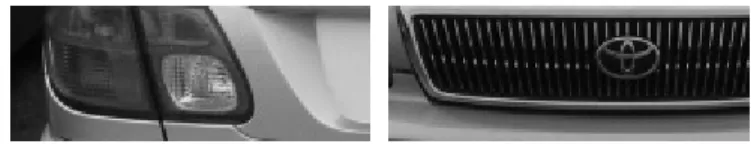
(11) projection of edge onto vertical and horizontal axes [5]. For the third step, character recognition, several algorithms have been also suggested, such as algorithms fulfilled by template matching methods [6] and neural networks [7]. Next, two main problems and the system flowchart will be expressed in this chapter.. 1.1 Problem Statements While the license plate recognition systems operate outdoors, it is easily perturbed by illumination variation or the complex texture of vehicles. Unfortunately, these disturbances will decrease the recognition accuracy. In order to design a robust license plate recognition system, it is necessary to analyze the disturbances and two important problems to be dealt with are proposed as following: 1.1.1 The disturbances caused by the vehicle headlamp or radiator The overall performance of license plate recognition would be highly affected by the license plate localization, which is the first stage of process. Some spatial masks have been proposed to strengthen the feature of license plate and apply histogram methods to detect its position. However, the vehicle headlamps and radiator often shows similar features like a license plate and then the algorithms could easily fail to locate the real license plate. Hence, how to ameliorate the disturbances resulted from the headlamps and radiator becomes an important problem.. 2.

(12) 1.1.2 The disturbances caused by the illumination variation and complex texture of vehicles In an outdoor environment like roadways or highways, the complex texture of vehicles and the varying illumination easily cause the extracted character image to be vague. The same problem also exists when a license plate is dirtied. As a result, the extracted characters will be over-segmented or under-segmented, which will reduce the recognition accuracy of the extracted characters. Therefore, it is also an important topic how to cope with the above problem to make the character recognition robustly is also an important topic. In order to improve the above drawbacks, this paper employs the row differential analysis method to reject the disturbances caused by the vehicle headlamp or radiator, which will be introduced in next chapter. In addition, an efficient character recognition approach incorporated with Dynamic Projection Warping methods will be developed in chapter 3.. 3.

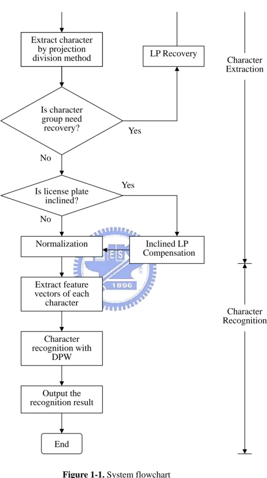
(13) 1.2 The flowchart of proposed system The algorithms of the proposed license plate recognition system in this paper are implemented by C language. They can be separated into three groups, license plate extraction, character extraction, and character recognition, which are all shown in the system flowchart Figure 1-1.. Begin. Input Car image (640×480 pixels). Convolute with spatial filter. LP Extraction. Moving average. Segment license plate candidate. Verification by RDA procedure. Not pass. Pass Extract character group by RDA procedure. 4.

(14) Extract character by projection division method. LP Recovery. Is character group need recovery?. Character Extraction. Yes. No Yes. Is license plate inclined? No Normalization. Inclined LP Compensation. Extract feature vectors of each character Character Recognition Character recognition with DPW. Output the recognition result. End Figure 1-1. System flowchart. 5.

(15) Chapter 2 The License Plate Extraction and Character Extraction. 2.1. Introduction Generally speaking, the procedure of license plate recognition system usually consists of three main steps, license plate extraction, character extraction and character recognition. Being the first step of vehicle license plate recognition system, the accuracy of license plate extraction directly affects the performance of the whole system. Therefore, the accuracy of license plate extraction should be dependable in this step. In the past two decades, several techniques of license plate extraction had been proposed such as color extraction method [8], symmetry [9], vertical edges [10], spatial mask [11] [12], and so on. In the real system, the proposed method has to be robust to various vehicles and complex environment. The color extraction method is not stable to various vehicles, especially to the white vehicle which has the same color as the license plate in Taiwan. The general symmetry transform method [9] which can reach the accuracy 93.6% has a impracticable computation cost, about a half minute, to apply to the real system. And the modified general symmetry transform method [9] which cost more than one second to extract out the license plate is still not suitable in. 6.

(16) the real system. The vertical edge matching method is good to the specific visual image which focuses on the license plate reliably. However, it is not easy to be stable in the complex environment with complicated background, which contains a large amount of vertical edges. Spatial mask method [11] [12] which is an efficient method of roughly extracting the license plate has an acceptable accuracy about 95%. However, the vehicle headlamps and radiator often shows similar features like a license plate in this method and then the algorithms could easily fail to locate the real license plate. Hence, how to ameliorate the disturbances resulted from the headlamps and radiator becomes an important problem. In this chapter, an improved license plate extraction method which combines spatial mask method and row differential analysis procedure that will be introduced later has been proposed. After a successful license plate extraction, the row differential analysis procedure is still helpful to searching character’s group. Then, by utilizing the projection method, characters can be extracted by its characteristics such as width, height, aspect ratio, the numbers, etc. Through a compensation of inclined license plate, each character will be normalized into 30×15 pixels for recognition.. 2.2. Spatial Mask When the license plate recognition system obtains a grey level image, the first. 7.

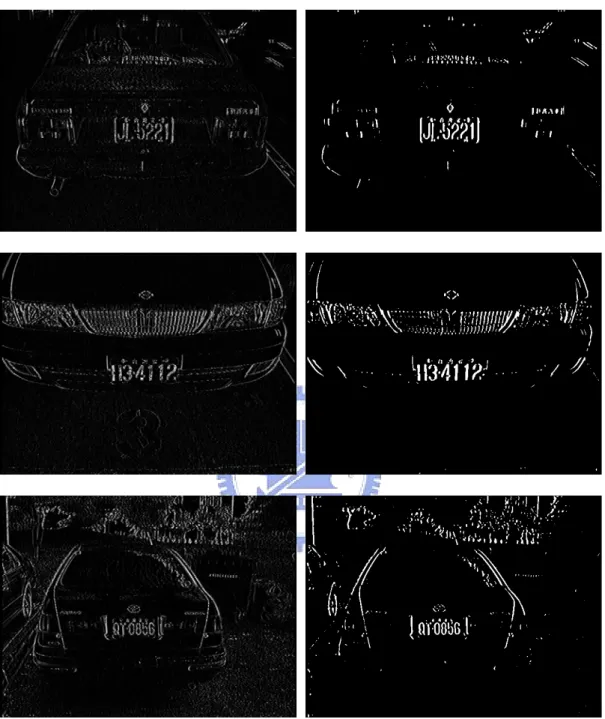
(17) goal is to extract out the license plate, which is regarded as a white rectangular metal plate and contains a character set including two alphanumeric characters and four numeric characters. The spatial filter method has been widely adopted in the step of license plate extraction [11], which requires a spatial mask to filter out character vertical strokes. Usually, the character stroke is about 5 pixels for a license plate of 110×40 pixels, which is the resulted image in our research. Figure 2-1 illustrates the distribution of a character vertical stroke in gray level image. Hence, a spatial mask h(k ) is designed to enhance the black vertical strokes from the white background is. shown as below h(k ) = {− 1, − 1, − 1,. 1,. 4,. 1,. − 1, − 1,. − 1}. (2.1). where k is an integer and − 4 ≤ k ≤ 4 . Let f be the original grey level image and g be the image in the spatial domain, the relationship between f and g can be expressed as below. g ( x, y ) =. 4. ∑ h(k ) f (x + k , y ). (2.2). k = −4. where f (x, y ) represents the grey level at the point ( x, y ) . Figure 2 illustrates the original grey level image and the image in the spatial domain.. 8.

(18) Figure 2-1. The grey level distribution of a character vertical stroke. Figure 2-2. (a) Original car images.. (b) Images of operation with spatial mask. 9.

(19) 2.3. Moving Average In this section, the moving average method which is adopted as the pre-process of license plate extraction will be introduced. In Figure 2-3(a), most pixels of the character are enhanced, but still many pixels of background are also enhanced. To remove the undesired noise from the image, the moving average method which consists of two main process, smoothing and binarilization, is usually employed. The smoothing operator represented as ⎡1 1 1⎤ 1⎢ M = ⎢1 1 1⎥⎥ 9 ⎢⎣1 1 1⎥⎦. (2.3). which is usually employed as a low-pass filter to smooth images. The image h’ after the moving average operation can be stated as following.. h′( x, y ) =. 1 1 1 ∑ ∑ g ( x + i, y + j ) 9 i =−1 j =−1. (2.4). To transfer the image h’ to binary, a threshold T has to be chosen first. For different lighting conditions, the threshold T should be different to make the best performance. Therefore, a dynamic threshold T is chosen as below,. T = ρ * max g ( x, y ). (2.5). ( x, y ). where ρ = 0.1 is an experiment value. Applying the dynamic threshold to h’ as as ⎧ 0 , if h′( x, y ) < T h ( x, y ) = ⎨ ⎩255 , if h′( x, y ) ≥ T. (2.6). where h is the binary image obtained from the binarilization of h and some binary. 10.

(20) images that are processed moving average are shown in Figure 2-3(b).. Figure 2-3. (a) Input images.. (b) Results of moving average. 11.

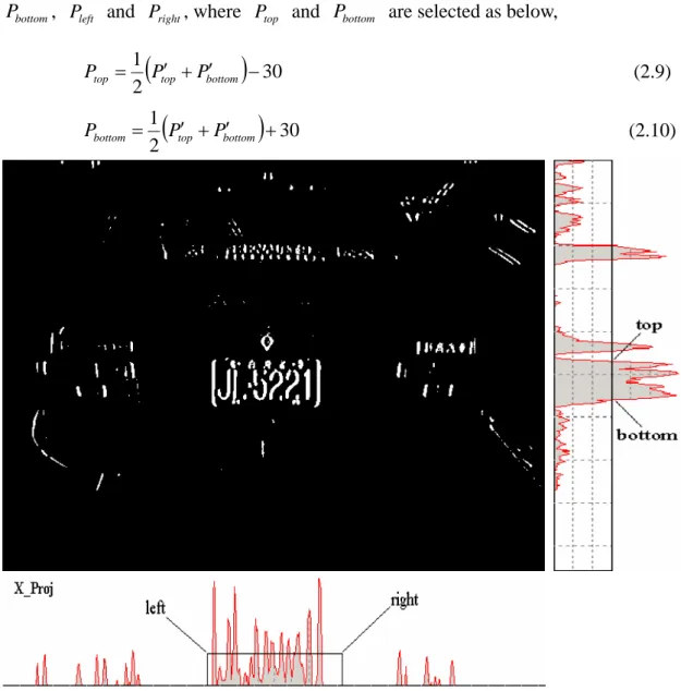
(21) 2.4. License Plate Candidate Segmentation Generally speaking, no matter what kind of car is, the license plate is mounted in the lower part of a car. Because of this property, searching license plate in the direction from the bottom toward the top of input image could be easier and more efficient. It would be better to say that the lower part of image has few noises such as lamps, symbols, radiators, etc. Base on this concept, a method called projection extraction method is used to rough license plate segmentation and the y-axis projection of image such as Figure 2-4 is usually used to searching the vertical position of license plate. In this paper, the proposed system is focus on the range of are of license plate is from 90×30 pixels to 130×50 pixels. Consequently, given Figure. ′ 2-4 as an example, if the distance from detected license plate bottom Pbottom to ′ is greater than 20 and the projection accumulated detected license plate top Ptop. value of each row exceeds 30, the range from detected license plate bottom to top will be considered as the y-axis position of license plate. By utilizing the x-axis projection of the selected vertical range of image, the detected license plate left Pleft and detected license plate right Pright will be selected as below,. Pleft = max. i∈(1, 640. 159. X _ Proj[i + j ] )∑. (2.7). j =0. Pright = Pleft + 160. (2.8). where X _ Proj [i ] is the accumulated value of i-th column of the selected vertical. 12.

(22) range of image. To avoid the failed segmentation, the license plate candidate, Figure 2-5 is given as examples, of size 160 × 60 pixels is chosen with the boundaries Ptop ,. Pbottom , Pleft and Pright , where Ptop and Pbottom are selected as below, Ptop =. 1 ′ ) − 30 (Ptop′ + Pbottom 2. Pbottom =. (2.9). 1 ′ ) + 30 (Ptop′ + Pbottom 2. (2.10). Figure 2-4. Rough license plate segmentation by projection. Figure 2-5. License plate candidates. However, sometimes the proposed method segments an incorrect license plate candidate such as lamps, radiators, etc. shown in Figure 2-6. Therefore, this paper also 13.

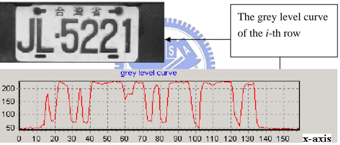
(23) proposed a procedure which will be introduced later to verify whether the candidate possesses license plate or not is necessary.. Figure 2-6. Incorrect license plate candidates. 2.5. Row Differential Analysis Procedure When the license plate candidate region was generated, a novel method, called row differential analysis procedure, will be used to verify whether the candidate region possesses license plate or not. Actually, the row differential analysis procedure verifies the candidate region by the configuration of the license plate and the stroke of characters in it. First, the candidate region can be defined as f (x, y ) where. [. x ∈ Pleft , Pright. ]. [. ]. and , y ∈ Ptop , Pbottom . The row differential analysis procedure will. take the differential operation from Pleft to Pright in each line and line by line from Ptop to Pbottom . The rising edge and falling edge of each line will be detected. simultaneously and the piece of character exists from falling edge to rising edge. Figure 2-7 illustrates the grey level curve of the row which crosses the license plate characters. Sequentially, it is necessary to record the length lk,i of each piece k of character and gather the statistic of the quantity Ni of piece of character in each line i. Due to the character of registration number, different stroke width will be assigned a 14.

(24) corresponding weight value as ⎧ 0 , as l k,i < L min , or l k,i > L max ⎪ w(l k,i ) = ⎨ 1, as L min ≤ l k,i < L threshold ⎪2 , as L threshold ≤ l k,i < L max ⎩. (2.11). where w(lk,i) represents weight value according to different length lk,i in k-th piece of i-th line. Lmax, Lmin and Lthreshold are threshold of length and their experiment value are. about 22, 2, 7 pixels respectively. Figure 2-8 and Figure 2-9 show the pieces with positive weight of several license plate candidates.. The grey level curve of the i-th row. Figure 2-7. The grey level curve of the i-th row. 15.

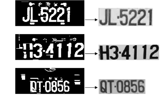
(25) Firgure 2-8. (a) correct license plate candidates (b) processed images. Firgure 2-9. (a) incorrect license plate candidates (b) processed images. According to the record of length lk,i of each piece k of i-th line, a statistic Gi which sums up the weight values is defined as (2.12) Ni. G i = ∑ w(l k,i ). (2.12). If the i-th line of license plate candidate region exists license plate, the value of the statistic Gi and the quantity Ni will be restricted to a range. For a ideal license plate image with no disturbance the range is from 6 to 13. However, a real system contains disturbances more or less, the range 4 to 20 instead of the ideal range is used in the. 16.

(26) proposed system. In other words, if the value of the statistic Gi and the quantity Ni of a license plate candidate satisfies the restriction, it will be considered that the i-th row crosses the license plate. If a row group can be considered crossing a license plate, the license plate candidate region could pass the RDA procedure such as the three candidates shown in Figure 2-8. It means the vertical range of license plate has found and the license plate detection will be stop. Furthermore, the position of x-axis can also be found by the projection of in the vertical range of the image which is processed by RDA procedure. Figure 2-10 shows three character group images extracted from license plate candidates. Otherwise, next license plate candidate region will be verified until the whole image is searched comprehensively. Figure 2-9 shows two examples which are segmented as license plate candidates are rejected by RDA procedure.. Figure 2-10. Extracted character group. 17.

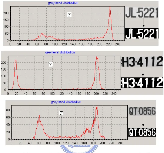
(27) 2.6 Binarilization After extracting the character group from the rough license plate, the binarilization process is usually employed as the pre-process of character extraction. Nevertheless, for different lighting conditions to have a best result the threshold should be different. Many methods of choosing the threshold from a grey level image such as binarilization by average, Ostu’s method [13], etc. According to the grey level distribution of extracted character group image, three examples are given in, the threshold used in this paper is a dynamic value, which is selected by the following steps. Suppose the extracted character group image, denoted as f (x, y ) , with m×n pixels, each pixel can be classified to either higher grey level class H or lower grey level class L, and the number of pixels in H is equal to L. Let σ H and σ L be the average grey level of H and L respectively, the threshold T is selected as (2.12) and the binary character group image R can be obtained from (2.13).. 1 (σ H + σ L ) 2 ⎧255 , if f ( x, y ) < T R ( x, y ) = ⎨ ⎩ 0 , if f ( x, y ) ≥ T. T=. (2.12) (2.13). Three examples of binary images are shown in Figure 2-11.. 18.

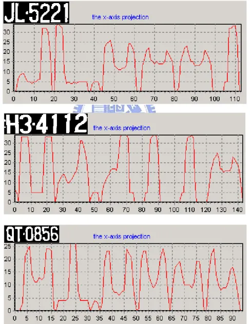
(28) Figure 2-11. the grey level distribution of character groups and the related binary. images.. 2.7 Character Extraction by Projection Method Projection method [14] calculates the number of pixels with the grey level 255 of each column, called column accumulated value, in the binary character group image. The vertical projection curves of three examples are shown in Figure 2-12. In the conditions with few disturbances, the column accumulated value will be equal to. 19.

(29) zero when the column contains no character. This kind of column will be considered as the division columns of characters. In the practice, columns with the column accumulated value that tends to zero and is a local minimum will be considered as the division columns of characters and each character can be extracted by these division columns.. Figure 2-12. the x-axis projection of binary character group images. Since the characters extracted out from different license plates are generally in 20.

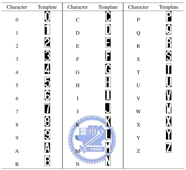
(30) different sizes which will make the character recognition more difficult, it is necessary to normalize the characters to a fixed size. By using the normalization method, all the characters processed in this paper is normalized to 30×15 pixels each, such as the character templates in Table 2-1. However, the images received by CCDs often contain undesired noise caused by varying illumination, blurred effect, dirty plate, and fragmented characters. As a consequence, it is rather difficult to perfectly extract the characters out, and most importantly, the recognition rate may be reduced to a certain level. To tackle the above problem, this paper proposes a new method, called dynamic projection warping (DPW), which will be introduced in the next chapter.. 21.

(31) Table 2-1. Normalized character templates. Character. Template. Character. Template. Character. 0. C. P. 1. D. Q. 2. E. R. 3. F. S. 4. G. T. 5. H. U. 6. I. V. 7. J. W. 8. K. X. 9. L. Y. A. M. Z. B. N. Template. 2.8 License Plate Recovery and Inclined License Plate Compensation When characters are extracted out, some additional and necessary information of license plate and characters are also obtained. Given Figure 2-13 as an example of license plate recovery [15], if any boundary of character is on the boundary of the extracted character group image, it means that perhaps some pixels of the character are outside the character group image. Consequently, that boundary of character group image will be extended one pixel and characters will be extracted by vertical 22.

(32) projection division method again. Repeat the above until every character is well-extracted.. Figure 2-13. License plate recovery. Due to the angle of camera capturing images, the extracted license plate is sometimes inclined with a small angle less than 10°. In order to have a better character recognition rate, an inclined license plate compensation procedure [2] is required. Let R p be the inclined license plate with its width wR and let ( xc , yc ) be the center of R p . In addition, let D R be the height difference between the centers of the first and the last characters of R p . Then, the compensated license plate image R ′p can be obtained from the following equation. Figure 2-14 shows the example of. inclined license plate compensation. R ′p ( x, y ) = R p ( x, y − ( x − xc ) * DR / wR ). Figure 2-14. Inclined license plate compensation. 23. (2.14).

(33) Chapter 3 Character Recognition Based on DPW. After a successful license plate extraction and character extraction, the following step, character recognition, is a very important part in the LPR system. Dynamic Projection Warping method, called DPW, proposed in this paper is to recognize character robustly. In the beginning, what kind of method DPW is and why use DPW for recognition will be expressed first. Then, what kind of feature vector chosen in DPW will be stated. In the third section, dynamic programming, a main technique of DPW, will be introduced. In the last the complete algorithm with assumptions and some analysis will be explained in detail.. 3.1. Motivation Generally speaking, basic recognition method of recognizing the license plate characters could reach the recognition rate, 80% per character, for example 85% per character for the template matching method. However, the above recognition rate is only for well-extracted characters. In practice, it is often hard to extract the license plate characters perfectly in outdoor environments, like roadways or highways. Although several methods have been proposed and obtained better results in character. 24.

(34) extraction, there is still no one can promise to always get well-extracted characters. Some characters will be over-segmented or under-segmented under certain conditions, especially for the soiled characters, the dirty license plates, the blurred or over exposed license plate images, and so on. These characters usually have fragmented strokes, undesired shifted image, pared character images, or unwell-normalized images, etc. The recognition rate of these characters may be reduced to less than 70% per character for basic recognition method. Therefore, how to cope with the above problem is an important topic to make the character recognition robustly. The proposed method, Dynamic Projection Warping, which reaches the recognition rate 99% of character recognition in LPR system, would be introduced in this chapter.. 3.2 Feature Vector of Character Recognition Dynamic projection warping, called DPW in brief, is proposed to cope with the uncertain character boundaries and the unwell-extracted normalized characters which are shifted, pared, fragmented, etc. The basic concepts of DPW are choosing projection accumulated vector of characters as feature vectors and applying these to dynamic programming method for recognizing characters. This section introduce why choose the projection accumulated vector as the feature vector. After the normalization, suitable feature vectors, which represented by a set of. 25.

(35) character features, have to be adopted for describing the character patterns that will be recognized. Projection accumulated vectors which reduce the dimension from 2-D image to 1-D curve are often adopted to be feature vectors in many LPR researches [16]. It is simpler to cope with a 1-D curve and has less computation cost. Hsu, Lin, Mar, and Su proposed Grey Relation Grade Analysis [16] as the recognition method adopts the Normalized Column Accumulated Vector, NCAV in brief, as the feature vector of the character for recognition. The Normalized Column Accumulated Vector (NCAV) is defined as n. CAV (i ) = ∑ chr [i ][ j ]. (3.1). j=1. NCAV (i ) =. CAV (i ) m. ∑. (3.2). CAV ( j ). j. where chr, m×n pixels, 30×15 pixels for this paper, is the binary image of the extracted character and chr[i][j] is the binary value of pixel (i,j). By using NCAV, 30 ×1 in this paper, as the feature vector of the character, the character recognition is fulfilled by the grey relation theory. However the recognition rate 72% and the improved recognition rate 94% are both not suitable for a real system. In case characters such as “M” and “N”, “U” and “H”, etc. which have similar feature in the accumulation space easily failed in recognition. Besides images encounter shifting, paring, fragmenting, etc., directly make the recognition failed. Although NCAV which makes characters more ambiguous in accumulation space, it utilizes the accumulated 26.

(36) value, which is more robust to the random noise, as the features of a character. Hence it is necessary to propose another robust recognition method to improve the recognition rate by using the accumulated vector as the feature vector. In order to overcome the above problems, this paper proposed a method called Dynamic Projection Warping, DPW in brief. It uses Projection Accumulated Vector, PAV in brief, as the feature vector, which can be decomposed into Column Accumulated Vector, CAV in brief, and Row Accumulated Vector, RAV in brief, defined as 15 ⎧ ( ) = RAV i chr [i ][ j ] ∑ ⎪ ⎪ j=1 PAV (i ) = ⎨ 30 ⎪CAV (i − n ) = ∑ chr [k ][i − 30 ] ⎪⎩ j=1. (3.3). It is easy to find that CAV is a 15×1 vector and RAV is a 30×1 vector. Consequently, PAV is a 45×1 vector. Figure 3-1 and Figure 3-2 illustrates the RAVs and CAVs of each reference. With the use of PAV, the dimension of the characteristic vector is extended to 30+15=45. Consequently, the higher dimension makes the recognition easier and enough to classify different characters.. 27.

(37) Figure 3-1. The RAV curve of each reference character. Figure 3-2. The CAV curve of each reference character. 28.

(38) 3.3 Dynamic Programming Technique In this paper, the PAV is chosen as the character feature vector, which has been discussed in the previous section. Here, dynamic programming technique that plays an important role for character recognition will be proposed. Dynamic programming technique has been extensively used in many fields such as speech recognition [17], optimal control [18], etc. Besides, dynamic programming technique has been also applied to character recognition in this paper. To illustrate the applicability of character recognition, a typical problem, called the optimal path problem, will be stated and discussed here. An example to explain the fundamental concept of the optimal path problem is given in Figure 3.3, which consists of N points labeled orderly from 1 to N. Besides, the cost moving directly from the i-th point to the j-th point in one step is represented by a nonnegative function ς (i , j ) . The path from point 1 to point i may have many selections and leads to different costs. As a result, there should exist a minimum cost, denoted as ϕ (1, i ) .. 29.

(39) Figure 3-3. The minimum cost related to the optimal path Using traditional terminology, the decision rule for determining the next point to be visited after point i is called a “policy”. Since the policy determines the sequence of points traversed from the (fixed) originating point 1 to the destination point i, the cost is therefore completely defined by the policy and the destination point i. The question is what policy leads to the function ϕ (1,i ) . This principle of optimality, which is the basis of a class of computational algorithms for the above optimization problem, is according to Bellman [19], An optimal policy has the property that, whatever the initial state and decision are, the remaining decisions must constitute an optimal policy with regard to the state resulting from the first decision. 30.

(40) To put Bellman’s principle of optimality into a functional equation suitable for computation algorithms, consider first moving from the initial point 1 to an intermediate point j in one or more steps. The minimum cost, as defined, is ϕ (1, j ) . Since moving from point j to point i in one step incurs a cost ς ( j ,i ) , the optimal policy, which determines which intermediate point j to pass through, (should one exist) satisfies the following equation. ϕ (1, i ) = min[ϕ (1, j ) + ϕ ( j , i )]. (3.4). j. Generalizing (3.4) to the case in how to obtain the optimal sequence of moves and the associated minimum cost from any point i to any other point j, the following equation can be derived from (3.4). ϕ (i, j ) = min[ϕ (i, l ) + ϕ (l , j )]. (3.5). l. where ϕ (i, j ) is the minimum cost from i to j in as many steps as necessary. (3.5) implies that any partial, consecutive sequence of moves of the optimal sequence from i to j must also be optimal, and that any intermediate point must be the optimal point linking the optimal partial sequences before and after that point. To actually determine the minimum cost path between points i and j, in any number of steps, the following simple dynamic program would be used:. ϕ 1 (1, l ) = ς (1, l ). l = 1,2, K, N. ϕ 2 (1, l ) = min[ς (1, k ) + ς (k , l )]. k = 1,2,K, N. k. 31.

(41) l = 1,2, K, N M. ϕ S (1, l ) = min[ς (1, k ) + ς (k , l )]. k = 1,2,K, N. k. l = 1,2, K, N ⇒ ϕ (i, j ) = min ϕ s (i, j ). (3.6). 1≤ s ≤ S. where ϕ s (i, l ) is the s-step best path from point i to point l, and S is the maximum number of steps allowed in the path. For a well-known aircraft routing problem illustrates in Figure 3-4, a, b, c, … represent cities, and the numbers represent the fuel required to complete each path. Using the principle of optimality the minimum-fuel problem could be solved easily. First each minimum-fuel cost, ϕ (i, j ) , can be obtained by (3.6). For example,. ϕ (a, e ) = min[ς (a, b ) + ς (b, e ), ς (a, e ), ς (a, d ) + ς (d , e )] = 4. (3.7). ϕ (a, e ) = 4 can be obtained as above. Because any partial, consecutive sequence of moves of the optimal sequence from i to j must also be optimal, the optimal path which is illustrated in red with the minimum-fuel cost from city a to city i, ϕ (a, i ) = 7 , can also be obtained.. 32.

(42) Figure 3-4. Aircraft routing network and the minimum-fuel cost from city a to each other.. 3.4 Dynamic Projection Warping In the previous sections, PAV which represented by a set of projection accumulation features and dynamic programming technique have been discussed. This section discusses how to integrated dynamic programming technique with the feature vector PAV for character recognition. The first subsection states that how to apply dynamic programming technique to the PAV for character recognition. Next,. 33.

(43) consider the disturbances of real LPR system, some constraints is proposed to constraint the “path” discussed in the previous section. Combining these constraints, the DPW method becomes complete for character recognition. However, for some specific characters, the recognition rate isn’t good enough. Last subsection discusses the modified DPW which can reach a excellent recognition rate over 99%.. 3.4.1 Fundamental Concepts of DPW This subsection expresses the integration of dynamic programming and PAV for character recognition. The pattern recognition always utilizes either maximum correlation or minimum dissimilarity classifying patterns. Traditional template matching method uses the minimum dissimilarity to determine the recognition result, that shown in below, d (i, j ) = chr [i ][ j ] − ref [i ][ j ]. (3.8). 30 15. dϕ (chr , ref (k )) = ∑∑ d (i, j ) i =1 j =1. [. (3.9). ]. O = arg min(dϕ (chr , ref (k ))) k. (3.10). where chr and ref (k ) represent the extracted character image and k-th reference character image in the database, respectively, d (i, j ) is the dissimilarity function of pixels between two character images, dϕ (chr, ref (k )) is the total dissimilarity between two character images, and O represents the output of recognition result. From 34.

(44) (3.8), it is obvious that template matching method only considers the dissimilarity of each pixel in the same coordinates between chr and ref. However, when the character extraction is disturbed by undesired noise, the extracted characters including shifting, paring, partially fragmenting, etc. will make the character recognition failed. Therefore, considering the adjacent pixels is necessary. Before formal introduction of the fundamental concept of DPW, for convenience, the CAV and RAV of a character respectively denoted as ϕ xc and ϕ xr , shown in (3.11). 30 ⎧ ( ) ( ) = = ϕ i RAV i chr [i ][ j ] ∑ xr x ⎪⎪ j =1 PAVx (i ) = ⎨ 15 ⎪ϕ xc (i − 30) = CAVx (i − 30 ) = ∑ chr [k ][i − 30] j =1 ⎩⎪. (3.11). The CAV and RAV of reference characters are respectively denoted as ϕ yc and ϕ yr , shown in (3.12). 30 ⎧ ( ) ( ) = = ϕ i RAV i ref [i ][ j ] ∑ yr y ⎪⎪ j =1 PAV y (i ) = ⎨ 15 ⎪ϕ yc (i − 30) = CAV y (i − 30 ) = ∑ ref [k ][i − 30] j =1 ⎩⎪. (3.12). Ignoring the shifting, scaling, paring and fragmenting of the extracted character images caused by disturbances, d (i, j ) , dϕc (chr, ref (k )) , dϕr (chr, ref (k )) and. dϕ (chr, ref (k )) will be defined as (3.13), (3.14), (3.15) and (3.16) d (i, j ) = PAVx (i ) − PAVy ( j ) , i = j. (3.13). 30. dϕr (chr , ref (k )) = ∑ ϕ xr (i ) − ϕ yr (i ) i =1. 35. (3.14).

(45) 15. dϕc (chr , ref (k )) = ∑ ϕ xc (i ) − ϕ yc (i ). (3.15). i =1. 45. dϕ (chr , ref (k )) = dϕr (chr , ref (k )) + dϕc (chr , ref (k )) = ∑ d (i, i ). (3.16). i =1. where d (i, j ) is the dissimilarity function of row or column accumulated values between two character images, dϕc (chr, ref (k )) and dϕr (chr, ref (k )) represent the total dissimilarity between two RAVs and CAVs, respectively, and dϕ (chr, ref (k )) is the total dissimilarity between two PAVs. , and the output O still can be obtained by (3.10). In the Figure 3-5, dϕc (chr, ref (k )) can be calculated by summing up each d (i, j ) corresponding to the grid point along the “path”, denoted as P.. Figure 3-5. The “path” of (3.15). 36.

(46) Unfortunately, the extracted character images usually contain more or less disturbances which cause the images shifted, scaled, pared and fragmented. The disregard of the effect of disturbances makes the recognition method doesn’t robust to disturbances and causes a lower recognition rate. Consequently, the “path” has to be changed when the extracted character image contains disturbance. Nevertheless how to reasonably and automatically find the “path” becomes a new problem. An example to explain how to choose the path is given in Figure 3-6, which illustrated an undesired character image, the under “Z”, which is normalized, over-extracted disturbances in the left two columns and under-extracted right two columns of the upper “Z” in Figure 3-6. It is apparent that ϕ xc which is shown below is almost a curve shifted two columns from ϕ yc .. ϕ xc (i ) = ϕ yc (i − 2) ,3 ≤ i ≤ 15. (3.17). Hence, the “path” in Figure 3-5 should be replaced by P’ which is illustrated in Figure 3-7.. 37.

(47) Figure 3-6. A comparison between the reference character and. the shifted character image and their related CAVs.. Figure 3-7. The “path” of a shifted input ϕ xc. 38.

(48) Figure 3-8 which illustrated another undesired character image is another example. The under “Z” is also an undesired character image which is normalized and under-extracted the left four columns. The CAV of the under “Z” can be stated as (3.18). ⎛. ⎡ 15 ⎤ ⎞ ⎟⎟ ,1 ≤ i ≤ 15 ⎣15 − 3 ⎥⎦ ⎠. ϕ xc (i ) = ϕ yc ⎜⎜ (i − 2) * ⎢ ⎝. (3.18). Thus, the “path” in Figure 3-5 should be replaced by P” which is illustrated in Figure 3-9.. Figure 3-8. A comparison between the reference character and the. pared character image and corresponding CAV.. 39.

(49) Figure 3-9. The “path” of a shifted input ϕ xc. Now, the main disturbances, which resulting from character extraction and normalization such as shifting, paring, and scaling, had been discussed. According to the above examples, each kind of character image has its related path to map the corresponding CAV to the CAV of reference image. Each path can be decomposed into three kinds of path, P1, P2 and P3, shown in Figure 3-10. Therefore, these three kinds of path are chosen as the fundamental types that will compose all the paths after.. 40.

(50) Figure 3-10. Three allowed sub-path in DPW. 3.4.2 Basic Dynamic Projection Warping. In the previous sections all the fundamental concepts and techniques, feature vectors, dynamic programming technique, the “path”, fundamental paths, etc., had been introduced, the character recognition method, dynamic projection warping, will be discussed here. Dynamic projection warping method is a method that can automatically choose the optimal mapping way, the “path”, between PAVx and the PAVy of each reference character image. By utilizing the dissimilarity, which is considered as the cost of a path, related to the path between PAVx and each PAVy, the input character can be classified to a suitable class by the minimum dissimilarity. The function d (i, j ) is denoted as the partial dissimilarity between two feature vectors and represents the partial cost of a path when the path goes through the grid point (i, j ) . Consequently, each partial dissimilarity d r (i, j ) and d c (i, j ) have to be respectively calculated as 41.

(51) (3.19) and (3.20).. d r (i, j ) = ϕ xr (i ) − ϕ yr ( j ) ,1 ≤ i, j ≤ 30 i, j ∈ N. (3.19). d c (i, j ) = ϕ xc (i ) − ϕ yc ( j ) ,1 ≤ i, j ≤ 15 i, j ∈ N. (3.20). After defining the partial dissimilarity, the cost of each path, dϕr (chr , ref (k )) ,. dϕc (chr , ref (k )) and dϕ (chr , ref (k )) , which represents the entire dissimilarity extracted character image and k-threference character image can be computed as (3.21), (3.22), and (3.23), d ϕr (chr , ref (k )) = dϕc (chr , ref (k )) =. ∑ d (i, j ). (3.21). ∑ d (i, j ). (3.22). (i , j )∈Pr. (i , j )∈Pc. r. c. dϕ (chr , ref (k )) = dϕr (chr , ref (k )) + dϕc (chr , ref (k )). (3.23). where Pr is the related minimum cost path, from beginning point to ending point, between ϕ xr and ϕ yr and Pc is the related minimum cost paths, from beginning point to ending point, between ϕ xc and ϕ yc . By utilizing dynamic programming technique, the minimum cost paths could be found feasibly with two constraints, called beginning region and ending region constraint and legal path constraint, which are illustrated in Figure 3-11. The size of ϕ r and ϕ c is denoted as Tr=30, and Tc=15, respectively. Figure 3-11, which only shows a concept of the two constraints, uses T to represent the size of ϕ x and ϕ y .. 42.

(52) Figure 3-11. The legal region of the path. . Beginning region and ending region constraint For an over-extracted character image which contains several rows or columns of. disturbances which are not a part of the desired character image. The disturbances may appear in the left, right, top, or bottom. For an under-extracted character image which is pared several rows or columns of desired character image. The pared rows or column may also in the left, right, top, or bottom. Reviewing Figure 3-6 to explain the concepts of beginning region and ending region, the under “Z” in Figure 3-6 is an example of an over-extracted character image which contains two-column disturbance 43.

(53) in the left side and is pared two-column in the right side. Therefore, the beginning point of the path P’, which is discussed before, is shifted from (1,1) to (3,1) and the ending point is shifted from (15,15) to (15,13) . It can be found that the beginning point is on the line j=1 when the character image is over-extracted. How far away from the beginning point to the point (1,1) represents the number of columns over-extracted in left side of character image. To make the DPW robust to over-extracted character image, the region of beginning point, called beginning region and denoted as RBx , under the over-extracted condition includes xo1 beginning points shows in (3.24). R Bx = {(i, j ) j = 1,1 ≤ i ≤ xo1 } , i, j ∈ N. (3.24). where xo1 is an experiment value that depends on the reliability of character extraction step. In other words, if the number of over-extracted columns in the left side of extracted character image is usually smaller than a constant, xo1 , then xo1 will be chosen as the maximum tolerance of over-extracted tolerance of over-extracted disturbance. Here, the value two of xo1 is selected by experiments. The same method applying to the right side of extracted image, the parameter xo 3 is selected two, which equals to xo1 . The region of endpoint, called ending region and denoted as R Ex , under the over-extracted condition includes Tc- xo 3 ending points shown in (3.25),. 44.

(54) R Ex = {(i, j ) j = Tc , Tc − xo 3 < i ≤ Tc } i, j ∈ N ,. (3.25). where Tc which equals to 15 represents the size of ϕ c . If ϕ xc and ϕ yc exchanges with each other, the beginning point of the new path is at (1,3) and the ending point is at (13,15) . It can be found that “an image over-extracted from the other image” is the same as “an image under-extracted from the other image”. Therefore, by utilizing the symmetry of i=j, RBx and R Ex under the pared condition can be chosen as (3.26) and (3.27) R By = {(i, j ) i = 1,1 < i ≤ y o1 } i, j ∈ N ,. (3.26). R Ey = {(i, j ) i = Tc , Tc − y o 3 < j ≤ Tc } i, j ∈ N ,. (3.27). Thus, to make the DPW method robust to both over-extracted character image and under-extracted one, the beginning region and the ending region are defined as below.. RB = RBx ∪ RBy. (3.28). RE = REx ∪ REy. (3.29). Applying the same concepts to ϕ r , (3.28) and (3.29) still holds. Table 3-1 shows the important experiment parameters of ϕ c and ϕ r .. 45.

(55) Table 3-1 The value of important parameters of RB and RE. . Parameter. Experiment value for ϕ c. Experiment value for ϕ r. xo1. 2. 3. xo3. 13. 27. yo1. 2. 3. yo3. 13. 27. Legal path constraint In Figure 3-11, the legal region R which constraints the legal path of mapping a. ϕ c to another or mapping a ϕ r to another is limited by six lines. How to define the six lines of ϕ c will be stated in detail, and applying the same concepts to ϕ r , the six lines corresponding to ϕ r can be selected, too. Considering a worst case of over-extracted character image in this paper, which over extracted xo1 columns in the left side and xo3 columns in the right side, the related path will has an average slope from beginning point to ending point as m L1 = m L2 =. Tc 15 = Tc − xo1 − xo 3 11. (3.30). which is the maximum slope legal path. Therefore, the slope of L1 and L2, m L1 and. mL2 , are given by (3.30). Considering another worst case of under-extracted character image in this paper, which under extracted yo1 columns in the left side and yo3 columns in the right side, the related path will has an average slope from beginning. 46.

(56) point to ending point as m L3 = m L4 =. Tc − x o1 − xo 3 11 = Tc 15. (3.31). which is the minimum slope of legal path. Hence, the slope of L3 and L4, mL3 and. mL4 , are give by (3.31). The legal path region is still limited by two lines, L5 and L6, which are parallel to the line i=j. For general extracted character images, the slope of corresponding path should equals to 1, which is adopted as the slope of L5 and L6. However, encountering disturbances, the path will move a short distance from i=j. The appearance is shown as (i − xo 2 ) ≤ j ≤ (i + y o 2 ). (3.32). where both xo2 and yo2 equal to an experiment value, xo2 = yo2 = 4. Summing up the above constraints, the legal region R of ϕ c , denoted as Rc, is shown in (3.33). ⎧ ⎫ 15 15 i + 2 < j < (i − 15) + 13 ⎪ ⎪ 11 11 ⎪ ⎪ 11 11 ⎪ ⎪ Rc = ⎨(i, j ) , (i − 2) < j < (i − 13) + 15⎬ i, j ∈ N 15 15 ⎪ ⎪ ,i − 4 < j < i + 4 ⎪ ⎪ ⎪ ⎪ ⎩ ⎭. (3.33). By utilizing the same concepts from defining Rc, both xo2 and yo2 are chosen 6 and the legal region R of ϕ r , denoted as Rr, is shown in (3.34), ⎧ 30 30 (i − 30) + 27 ⎫⎪ i+3< j < ⎪ 24 24 ⎪ ⎪ 24 24 ⎪ (i − 27 ) + 30⎪⎬ i, j ∈ N Rc = ⎨(i, j ) , (i − 3) < j < 30 30 ⎪ ⎪ ,i − 6 < j < i + 6 ⎪ ⎪ ⎪ ⎪ ⎩ ⎭. 47. (3.34).

(57) Combining the two constraints with basic DPW, the complete character recognition method, called DPW, is shown as three steps below. . Step 1. Calculate the dissimilarity between two columns or two rows.. d r (i, j ) = ϕ xr (i ) − ϕ yr ( j ) ,1 ≤ i, j ≤ 30 d c (i, j ) = ϕ xc (i ) − ϕ yc ( j ) ,1 ≤ i, j ≤ 15 . (3.35). (3.36). Step 2. Calculate the total dissimilarity between extracted character image and the k-th reference character image. d ϕr (chr , ref (k )) = min Pr ∈Rr. d ϕc (chr , ref (k )) = min Pc ∈Rc. ∑ d (i, j ). (3.37). ∑ d (i, j ). (3.38). (i , j )∈Pr. (i , j )∈Pc. r. c. d ϕ (chr , ref (k )) = d ϕr (chr , ref (k )) + d ϕc (chr , ref (k )) . (3.39). Step 3. Recognize extracted character image by the minimum dissimilarity. d ϕ (chr , ref (k )). [. ]. O = arg min(d ϕ (chr , ref (k ))) k. (3.40). 3.4.3 Modified Dynamic Projection Warping. In the previous section DPW, the proposed character recognition method, has been introduced. It is useful to classify license plate character but some ambiguous character pairs. Table 3.2 shows the most similar reference character image of each one in the database except for itself and the corresponding dissimilarity calculated by. 48.

(58) DPW method. By experiments, if the dissimilarity between two characters is smaller than 60, the two characters are ambiguous to each other and the dissimilarity greater than 100 implies the two characters are far away in the DPW domain. From Table 3-2, it is clear to see that some characters are ambiguous in the DPW domain such as “E” and “F”, “M” and “N”, “A” and “V”, etc. Therefore, DPW has to be modified to improve the performance of character recognition. Table 3-2 The most similar reference character image of each one in the. database except for itself and the corresponding dissimilarity in the DPW space.. Char.. Most similar. Dis.. Char. Most similar. Dis.. Char.. Most similar. Dis.. 0. U. 50. C. G. 65. P. F. 67. 1. I. 72. D. R. 55. Q. 8. 67. 2. Z. 74. E. F. 28. R. D. 55. 3. S. 77. F. E. 28. S. 9. 56. 4. 3. 135. G. 6. 55. T. 7. 85. 5. S. 79. H. U. 49. U. H. 49. 6. G. 55. I. 1. 72. V. A. 51. 7. Z. 81. J. 3. 109. W. N. 61. 8. 9. 58. K. R. 62. X. A. 57. 9. S. 56. L. F. 120. Y. T. 91. A. V. 51. M. N. 38. Z. 2. 75. B. 8. 65. N. M. 38. 49.

(59) Now, a modified character recognition method, called modified DPW, is proposed to improve the performance of DPW. To enhance each partial feature of each character, the feature vectors are divided into three vectors as below, 5*l ⎧ ( ) ( ) ϕ RAV i = i = ∑ chr [i][ j ] l rl ⎪⎪ j=5*(l −1) PAVl (i ) = ⎨ 10*l ⎪CAVl (i − n ) = ϕ cl (i − n ) ∑ chr [k ][i − 30] j=10*(l −1) ⎩⎪. ,1 ≤ i ≤ 30 (3.41) ,31 ≤ i ≤ 45. where l=1,2,3 and PAV1, PAV2, and PAV3 satify (3.42), PAV (i ) = PAV1 (i ) + PAV2 (i ) + PAV3 (i ). (3.42). Applying each PAVl to the equation from (3.35) to (3.38) of proposed DPW to obtain. the. d ϕrl (chr , ref (k )). corresponding. and. d ϕcl (chr , ref (k )) ,. the. dϕ (chr , ref (k )) , which is used to recognized character image, in (3.43) will be adopted. 3. [. ]. d ϕ (chr , ref (k )) = ∑ d ϕrl (chr , ref (k )) + d ϕcl (chr , ref (k )). (3.43). l =1. Then, applying all the dϕ (chr , ref (k )) to (3.40), the character whose reference image has the minimum dissimilarity between extracted character image will be consider as the recognition result. Analyzing the most similar reference character image of each one in the database except for itself and the corresponding dissimilarity in modified DPW space, which are shown in Table 3-3, it is obvious that the modified DPW is better than DPW. After the modification, most dissimilarity of each character pair is greater than 60. The only two character pairs are “0” and “D”, and “8” and “B”. Then,. 50.

(60) the experiment results of DPW and modified DPW for character recognition will be shown in chapter 4. Table 3-3 The most similar reference character image of each one in the. database except for itself and the corresponding dissimilarity in the modified DPW space.. Char.. Most similar. Dis.. Char. Most similar. Dis.. Char.. Most similar. Dis.. 0. D. 59. C. G. 61. P. F. 75. 1. 7. 168. D. 0. 59. Q. 0. 75. 2. Z. 76. E. F. 63. R. B. 70. 3. 9. 95. F. E. 63. S. 9. 78. 4. A. 166. G. C. 61. T. Y. 82. 5. 9. 84. H. M. 85. U. D. 81. 6. B. 63. I. X. 136. V. W. 127. 7. Y. 102. J. 3. 121. W. V. 127. 8. B. 48. K. X. 128. X. Z. 123. 9. S. 79. L. E. 127. Y. T. 83. A. 8. 142. M. N. 65. Z. 2. 75. B. 8. 48. N. M. 65. 51.

(61) Chapter 4 Experiments of Proposed System. In the previous chapters, the three main steps of the proposed LPR system are introduced. In this chapter, some experiment results of each step will be expressed such as the accuracy of license plate extraction, the recognition rate of basic DPW and modified DPW with different feature vectors, the recognition rates of different recognition methods.. 4.1 License plate extraction Experiments have been implemented to test the efficiency of the proposed vehicle license plate recognition system to recognize Taiwanese vehicle license plate in input grey-level image, which is in the size 640×480 pixels. The 262 input images which include dirty plates and dim images are taken under varying illumination conditions. And the accuracy of license plate extraction about 98.9% (259/262) is better than the accuracy, about 95%, of conventional method extracted by spatial mask [12]. More examples of the accurate license plate extraction are given in Figure 4-1. Figure 4-2 shows the other three images failed in license plate extraction. The upper one is too dark to extract license plate and the license plate images of lower two. 52.

(62) are too small, about 60×20, for license plate extraction.. Figure 4-1. The input grey-level images and the extracted license plates. 53.

(63) failed. failed. failed. Figure 4-2. The three images failed in license plate extraction step. 54.

(64) 4.2 Character Recognition In this section some experiment results of dynamic projection warping including the recognition rates of different feature vectors, and the recognition rates by different recognition methods. The test data are the characters that extracted from the 259 license plate images mentioned in section 4.1. Therefore, there are 259×2=518 alphanumeric characters and 259×4=1036 numeric characters. The number of each alphanumeric character and numeric character is listed in Table 4-1 and Table 4-2, respectively.. Table 4-1 The number of each alphanumeric character extracted from input images Char. No.. Char. No.. Char. No.. Char. No.. Char. No.. 0. 9. 7. 30. E. 11. L. 19. T. 15. 1. 3. 8. 12. F. 20. M. 8. U. 10. 2. 19. 9. 13. G. 8. N. 9. V. 12. 3. 28. A. 15. H. 18. P. 17. W. 21. 4. 8. B. 10. I. 8. Q. 17. X. 9. 5. 11. C. 15. J. 38. R. 10. Y. 15. 6. 22. D. 17. K. 13. S. 13. Z. 15. 55.

(65) Table 4-2 The number of each numeric character extracted from input images Char. No.. Char. No.. Char. No.. Char. No.. Char. No.. 0. 91. 2. 115. 4. 69. 6. 102. 8. 132. 1. 101. 3. 95. 5. 109. 7. 103. 9. 119. 4.2.1 The recognition rates of basic DPW and modified DPW with different feature vectors In chapter 3, the recognition methods basic DPW and modified DPW had been introduced. The difference between these two methods is only the feature vector. It would be better to say that the feature vector of basic DPW, PAV, is equally divided into three parts, PAV1, PAV2 and PAV3, and each component of the feature vectors satisfies. PAV (i ) = PAV1 (i ) + PAV2 (i ) + PAV3 (i ). (4.1). where PAV (i ) is a row or column accumulated value as it mentioned before. Maybe someone would have the question of why the number three is selected. Here, some experiment results are shown to explain why divided the feature vector into three parts not two or else. Table 4-3 and Table 4-4 show the recognition rate of alphanumeric characters and numeric characters respectively. The suffixes of DPW in these Tables represent how many parts the feature vector divided into, for example. 56.

(66) DPW3 means that the feature vector is divided into three parts equally. In the last, from Table 4-5 which shows the total recognition rate of each modified DPW, it is obvious that DPW3 has the best recognition rate for recognizing license plate characters. Table 4-3 Recognition rate (%) of alphanumeric characters Char. DPW1. DPW2. DPW3. DPW4. DPW5. Char. DPW1. DPW2. DPW3. DPW4. DPW5. 0. 22. 100. 100. 100. 89. I. 88. 100. 100. 100. 100. 1. 100. 100. 100. 100. 100. J. 92. 92. 92. 92. 92. 2. 100. 100. 100. 100. 100. K. 100. 100. 100. 100. 92. 3. 89. 100. 100. 100. 100. L. 100. 100. 100. 100. 100. 4. 100. 100. 100. 100. 100. M. 88. 88. 88. 88. 88. 5. 100. 100. 100. 100. 100. N. 89. 100. 100. 100. 100. 6. 82. 95. 100. 100. 100. P. 100. 100. 100. 100. 94. 7. 100. 100. 100. 100. 100. Q. 94. 94. 100. 100. 100. 8. 83. 67. 83. 58. 67. R. 80. 90. 100. 100. 100. 9. 100. 92. 100. 100. 92. S. 100. 100. 100. 100. 100. A. 80. 100. 100. 100. 100. T. 93. 100. 100. 100. 100. B. 80. 90. 80. 70. 70. U. 100. 100. 100. 100. 100. C. 100. 100. 100. 93. 93. V. 83. 100. 100. 100. 100. D. 82. 82. 88. 65. 65. W. 48. 100. 100. 100. 100. E. 100. 100. 100. 91. 100. X. 89. 100. 100. 100. 100. F. 25. 80. 100. 75. 75. Y. 100. 100. 100. 100. 100. G. 100. 100. 100. 100. 100. Z. 100. 100. 100. 100. 100. H. 100. 100. 100. 89. 78. Total. 87.8. 96.1. 98.1. 94.8. 94.0. 57.

(67) Table 4-4 Recognition rate (%) of numeric characters Char. DPW1. DPW2. DPW3. DPW4. DPW5. Char. DPW1. DPW2. DPW3. DPW4. DPW5. 0. 98. 99. 100. 100. 100. 6. 95. 100. 100. 100. 99. 1. 100. 97. 99. 99. 99. 7. 100. 100. 100. 100. 99. 2. 97. 100. 100. 100. 100. 8. 97. 86. 100. 70. 60. 3. 100. 99. 100. 100. 99. 9. 98. 100. 100. 100. 96. 4. 100. 100. 100. 100. 100. 5. 100. 100. 100. 100. 100. Total. 98.5. 97.7. 99.9. 96.0. 94.0. Table 4-5 The recognition rates (%) of each modified DPW alphanumeric. numeric. total. DPW1. 87.8. 98.5. 94.9. DPW2. 96.1. 97.7. 97.2. DPW3. 98.1. 99.9. 99.3. DPW4. 94.8. 96.0. 95.6. DPW5. 94.0. 94.0. 94.0. 58.

(68) 4.2.2 The comparison between different recognition methods In this section, to compare the performance of proposed DPW method with the conventional recognition method, five recognition methods including conventional template matching method, modified template matching method [12], GRG method [16], the basic DPW method and the modified DPW method, are tested with the same 259 license plate images which mentioned in section 4.1. In Table 4-6, it is clear that the basic DPW is better than other conventional recognition method. After the modification, the recognition rate is improved and much better than others, especially for recognizing numeric characters. Table 4-6 The recognition rates (%) of conventional methods and proposed DPW alphanumeric. numeric. average. plate. DPW3. 98.1. 99.9. 99.3. 95.8. DPW1. 87.8. 98.5. 94.9. 73.4. 92.8. 93.6. 93.3. 71.9. 90.7. 88.2. 89.1. 48.3. 71.9. 57.3. 65.6. ×. Modified template matching method Template matching method GRG. 59.

(69) Chapter 5 Conclusion and Future Work. In general, the disturbances caused by the vehicle headlamp or radiator affect the license are the main disturbances in the license plate extraction step. Some spatial masks have been proposed to strengthen the feature of license plate and apply histogram methods to detect its position. However, the vehicle headlamps and radiator often shows similar features like a license plate and then the algorithms could easily make the license plate extraction fail. The proposed RDA procedure which is used to verify the license plate candidate not only improves the accuracy of license plate extraction but also helpful in character extraction. The license plate extraction by proposed method supplies a dependable accuracy about 99% (259/262) in practice. The disturbances caused by the illumination variation and complex texture of vehicles usually make the character extraction more difficult. Because of the more unwell-extracted characters lead to lower recognition rate in character recognition, a recognition method called DPW is designed to recognize the unwell-extracted characters. In the experiments it has an average recognition rate about 94.9% (1475/1554) is better than the other conventional methods. After the modification, the average recognition rate which is improved and reaches 99.3% is noticeably better. 60.

(70) than conventional methods, especially the accuracy 99.9% for numeric characters. Finally, the proposed recognition method using only addition operator, subtraction operator and absolute operation with the average recognition rate more than 99% is very suitable for hardware implementation. If the proposed LPR system were implemented by low cost hardware, it could be very popular and practicable in the related applications.. 61.

(71) References [01] T. Naito, T. Tsukada, K. Yamada, K. Kozuka, and S. Yamamoto, “Robust license-plate. recognition. method. for. passing. vehicles. under. outside. environment,” IEEE Trans. on Vehicular Technology, Vol. 49, pp. 2309-2319, 2000. [02] T.H. Wang, F.C. Ni, K.T. Li, Y.P. Chen,”Robust License Plate Recognition based on Dynamic Projection Warping,” IEEE International Conference on Networking, Sensing and Control, March., 2004. [03] Da-Shan Gao and Jie Zhou, “Car license plates detection from complex scene”, 5th International Conference on Signal Processing Proceedings, Vol. 2, pp. 1409-1414, Aug., 2000. [04] S.H. Park, K.I. Kim, K. Jung, and H.J. Kim, “Locating car license plates using neural networks”, Electronics Letters, Vol. 35, pp.1475-1477, Aug., 1999. [05] K. Kanayama, Y. Fujikawa, K. Fujimoto, and M. Horino, “Development of vehicle-license number recognition system using real-time image processing and its application to travel-time measurement,” IEEE Veh. Technol., pp. 798-804, 1991. [06] P. Comelli, P. Ferragina, M.N. Granieri, and F. Stabile, “ Optical recognition of motor vehicle license plates”, IEEE Trans. on Vehicular Technology, Vol. 44, pp.790-799, 1995. [07] M. Fahmy, “Automatic number-plate recognition: neural network approach”, Vehicle Navigation and Information Systems Conference, pp. 99-101, Aug., 1994. 62.

(72) [08] K. K. Kim, et al, ”Learning Based Approach of License Plate Recognition,” IEEE Signal Processing Society Workshop on Neural Networks for Signal Processing, vol. 2 ,pp 614-623, 2000. [09] Dong-Su Kim, et al, ”Automatic Car License Plate Extraction Using Modified Generalized Symmetry Transform and Image Warping,” ISIE CNF 2001 [10] Mei-Yu, Yong Deak Kim, ”An Approach to Korea License Plate Recognition Based on Vertical Edge Matching,” Systems, Man, and Cybernetics, 2000 IEEE International Conference on , Volume: 4 , 8-11 Oct. 2000 Pages:2975 - 2980 vol.4 [11] Jian-Yang, Zeng, “A research on Plate Localization, Preprocessing and Recognition of License Plate Recognition System,” T NCTU CLENG 1999 pt.7:3 [12] 趙慕霖, ”架構於數位訊號處理器之車牌辨識系統,” 國立交通大學電機與控制工程研究所, 2001. [13] N. Ostu, “A Threshold Selection Method from Gray-Level Histograms,” IEEE Transactions on System, Man, and, Cyber-netics, Vol. SMC-9, pp62-66, 1979 [14] 林泰良, “智慧型車牌定位與字串分割,” 國立台灣大學電機工程研究所碩士論文, 2000. [15] 陳麗奾, “在未設限環境下車牌的定位與辨識,” 國立台灣師範大學資訊教育研究所碩士論文, 1999. [16] Yen-Tseng Hsu, Chan-Ben Lin, Sea-Chon Mar, and Shun-Feng Su, “High Noise Vehicle Plate Recognition Using Grey System”, Journal of Grey System, Vol. 10, 63.

(73) No. 3, pp. 193-208, 1998. [17] Frank L. Lewis, Vassilis L. Syrmos, Optimal Control. [18] Lawrence Rabiner, Biing-Hwang Junag, Fundamentals of Speech Recognition, Prentice Hall Co Ltd., 1993. [19] R.E. Bellman, Dynamic Programming, Princeton University Press, Princeton, New Jersey, USA 1957.. 64.

(74)