WiMAX系統的基地台搜尋與鏈路之建立

國

立

交

通

大

學

電信工程學系

碩

士

論

文

WiMAX 系統的基地台搜尋與鏈路之建立

Cell Search and Initial Link Setup for WiMAX

Systems

研 究 生：陳慧珊

指導教授：蘇育德 博士

WiMAX 系統的基地台搜尋與鏈路之建立

Cell Search and Initial Link Setup for WiMAX

Systems

研 究 生：陳慧珊

Student：Hui-Shan Chen

指導教授：蘇育德 博士 Advisor：Dr. Yu T. Su

國立交通大學

電信工程學系碩士班

碩 士 論 文

A Thesis Submitted to

Department of Communication Engineering

College of Electrical and Computer Engineering

National Chiao Tung University

In Partial Fulfillment of the

Requirements for the Degree of

Master of Science

In Communication Engineering

Hsinchu, Taiwan, Republic of China

WiMAX 系統的基地台搜尋與鏈路之建立 研究生: 陳慧珊 指導教授: 蘇育德 博士 國立交通大學電信工程學系碩士班 中文摘要 基地台搜尋是細胞式行動通訊系統設計的一項很重要的議題。每個行動台開 機後第一項工作即是基地台搜尋與初步之鏈路建立。基地台下鏈信號一定有某個 通道負責傳送引導符元(pilot symbols)以供行動台用來做快速和可靠的訊號獲取 與同步。對OFDMA系統而言，訊號獲取與同步包含了框架偵測(frame detection)， 載波頻率同步，框架時差的粗調與微調以及通道的估計。有時候基地台會傳送另 外的引導符元用作基地台的辨認。但在WiMAX系統下，訊號獲取、同步與基地 台的辨認都必須在下鏈框架的第一個引導符元期間完成。 本文提供了一套WiMAX系統的基地台搜尋與初步連結建立的演算法。IEEE

802.16e標準訂定了114個不同的二元引導序列(binary pilot sequences)分別指派給

32個不同的基地台使用。這些引導序列由電腦收尋產生，沒有什麼數學結構，不 同的序列間之相關性也非常低，且只含在下載框架的第一個符元間。唯一比較特 殊的是其在時間軸上有近似的週期性。我們主要即是利用這重複週期性質和序列 間的低相關性來從事基地台搜尋與初步連結的建立。由於通道估計與序列同步有 必要同時完成，我們也應用了通道頻率響應在小區間的平滑性來驗證序列收尋之 正確與否。電腦模擬結果顯示我們所提出的基地台搜尋解決方案在複徑衰減通道 下有相當令人滿意的性能表現，而所需要的複雜度並不高。

Cell Search and Initial Link Setup for WiMAX

Systems

Student : Hui-Shan Chen Advisor : Yu T. Su

Department of Communications Engineering National Chiao Tung University

Abstract

Establishing a radio link in a WiMAX (IEEE 802.16e) system requires searching for and synchronizing the downlink known pattern (sequence) associated with the cell base station closest to the terminal in question. This process is often referred to as cell search and/or initial link setup and is perhaps the most critical radio receiver operation.

The synchronization process includes at least three major operations, namely, frame detection, carrier frequency offset estimation and fine symbol (frame) timing. In a multi-path fading environment, channel estimation is also called for during the synchronization phase. For a WiMAX system, these operations are accomplished with the aid of two kinds of pilot symbols. The first pilot symbol is common to all cells and segments but the second one is cell specific.

In this thesis, we present a complete solution for cell search and initial link setup for WiMAX system. The difficulty lies in the fact that there are more than 100 (114 in total) candidate cell specific pilot patterns with no inter-pattern algebraic and sta-tistical structure and relationship: the cross-correlations are uniformly low and the set of sequences are independent. The most useful property is their almost-periodicity in time domain. Our solution exploits this and other properties like Fourier transform representation of cyclic correlation and smoothness of the channel frequency response.

Numerical analysis and simulation results do verify that the proposed algorithms are efficient in complexity and more than satisfactory in performance.

Contents

English Abstract i

Contents iii

List of Figures v

1 Introduction 1

2 Downlink Subframe Structure of WiMAX 3

2.1 OFDM vs. OFDMA . . . 3

2.2 Basics of OFDMA frame structure . . . 5

2.3 Downlink preamble structure . . . 7

2.4 SUI channel model . . . 8

2.5 SCM channels . . . 9

3 Frame Detection and Carrier Frequency Offset Estimation 14 3.1 Frame detection . . . 14

3.2 Carrier frequency offset estimation . . . 17

4 Segment Decision and Cell Acquisition 26 4.1 Segment decision . . . 26

4.2 Group association: joint cell search and timing estimation . . . 28

4.3 Joint channel estimation and sequence identification . . . 34

5 Cell Search in the Presence of Large CFO 40

6 Conclusion 43

List of Figures

2.1 Time and frequency domain representations of OFDM waveforms [1]. . . 4

2.2 Block diagram of an OFDMA system with consecutive subcarriers assign-ment. . . 4

2.3 An OFDMA system with interleaved subcarriers. . . 5

2.4 OFDMA frame structure [2]. . . 6

2.5 Partial preamble modulation sequences for the 1K FFT mode [3]. . . 7

2.6 Preamble carrier-set for Segment 0 . . . 8

3.1 Operation flow chart of the cell search procedure. . . 20

3.2 WiMAX downlink frame structure and the corresponding time domain preamble sequence. . . 21

3.3 Normalized total correlation as a function of the initial sampling instant n. The down-link frame arrives at n = 500. The peak correlation occurs at n = CP duration; N = 1024 subcarriers , lcp= 64 bits. . . 22

3.4 Time domain preamble (pilot) symbol exhibits a repetitive structure. . . 23

3.5 Some typical values of the complex product y[n] = x[n]x∗_{[n + L] for} n : 0, 1, 2, . . . , (L − 1) . . . 24

3.6 The MSE performance of the proposed CFO estimator in an AWGN chan-nel; N = 1024 subcarriers and the cyclic prefix is 64-bit long.) . . . 25

4.2 The correlation magnitude Z1[n] between the received sample sequence

and the first sum-sequence at various lags. Subband energy detector out-put is maximized at the true locations; N = 1024 subcarriers and lcp = 64

bits. . . 29

4.3 The correlation magnitude Z2[n] between the received sample sequence and the 2nd sum-sequence at various lags; N = 1024 subcarriers, lcp = 64 bits. . . 30

4.4 Cell search procedures with and without group re-partition. . . 31

4.5 Probability of false cell detection in a SUI-3 channel. . . 33

4.6 Probability of false cell detection in a SCM channel. . . 33

4.7 Channel estimate by a correct preamble sequence. . . 36

4.8 Channel estimate by an incorrect preamble sequence. . . 37

4.9 Performances comparison between the noncoherent frequency domain matched filter bank (FDMFB) approach and the joint channel/sequence estimation (JCSE) method in a SUI-3 channel. . . 38

4.10 A simplified cell search procedure. . . 38

4.11 Performance of the direct cell identification approach in an SUI-3 channel (1024 subcarriers, 64-bit long CP). . . 39

4.12 Performance of the direct cell identification approach in an SCM channel (1024 subcarriers, 64-bit CP). . . 39

5.1 Cell search procedures without segmentation. . . 41

5.2 False cell detection probability of the DS-WOS approach in the presence of integer CFO; SUI-3 channel, 1024 subcarriers, 64-bit CP. . . 42

5.3 False cell detection probability performance of the DS-WOS approach in the presence of integer CFO; SCM channel, 1024 subcarriers, 64-bit CP. . 42

Chapter 1

Introduction

The IEEE 802.16e (WiMAX) standard provides specifications for an air interface for fixed, portable, and mobile broadband wireless access systems. The standard includes requirements for high data rate Line of Sight (LOS) operation in the 10 − 66 GHz range for fixed wireless networks as well as requirements for Non Light of Sight (NLOS) fixed, portable, and mobile systems operating in sub 11 GHz licensed-exempt band.

Because of its superior performance in multi-path fading wireless channels, Orthog-onal Frequency Division Multiplexing (OFDM) signaling is recommended in OFDMA Physical (PHY) layer modes of the 802.16 standard for operation in sub 11 GHz NLOS applications. OFDM technology has been adopted in other wireless standards such as Digital Video Broadcasting (DVB) and Wireless Local Area Networking (WLAN), and it has been successfully implemented in the compliant solutions.

A frame is about 3 ms long and starts with a cell-specific preamble which is 1 OFDMA (Orthogonal Frequency Division Multiplexing Access) symbol long. In order to properly demodulate the subsequent data signals, an SS (Subscriber Station) should detect the ID of the cell which is best to be associated with, as well as synchronize its oscillator frequency and clock timing with that of received signal.

The purpose of this thesis is to propose feasible solutions for initial link setup in a WiMAX system. Link setup requires that a terminal be synchronized with the downlink preamble of a close-by cell base station. As each cell is divided into three segments

and transmits in each segment a cell (segment) specific preamble (pilot) sequence, the terminal must be able to recognize and synchronize with this sequence. To accomplish this goal, it searches, amongst the known 114 candidate sequences, for the unique one that associated with the segment in which the terminal resides. Such a cell-search process involves more than sequence recognition, it includes frame detection/synchronization, frequency synchronization, and channel estimation, i.e., all necessary operations in the “outer receiver” part of a WiMAX receiver.

The rest of this thesis is organized as follows. Chapter 2 gives a brief introduction of the downlink frame structure and channel models in WiMAX. The main algorithms that include frame detection, carrier frequency offset estimation, timing recovery, channel estimation and cell determination will be expanded in chapter 3 and chapter 4. In chapter 5, integer carrier frequency offset is considered and detection procedures will be modified. Finally, the conclusion is given in chapter 6.

Chapter 2

Downlink Subframe Structure of

WiMAX

The term WiMAX (Worldwide Interoperability for Microwave Access) has become synonymous with the IEEE 802.16 Wireless Metropolitan Area Network (MAN) air interface standard. In its original release the 802.16 standard addressed applications in licensed bands in the 10 to 66 GHz frequency range. Subsequent amendments have extended the 802.16 air interface standard to cover non-line of sight (NLOS) applications in licensed and unlicensed bands from 2 to 11 GHz bands. Filling the gap between Wireless LANs and wide area networks.

2.1

OFDM vs. OFDMA

IEEE 802.16 specifies two classes of OFDM systems: one simply identified as OFDM, the other OFDMA.

Orthogonal frequency division multiplexing (OFDM) is a multi-carrier trans-mission technique that has been recently recognized as an excellent method for high speed bi-directional wireless data communication. OFDM effectively squeezes multiple modulated carriers tightly together, reducing the required bandwidth but keeping the modulated signals orthogonal so they do not interfere with each other. OFDM is similar to FDM but much more spectrally efficient by spacing the sub-channels much closer together (until they are actually overlapping). This is done by finding frequencies that

Figure 2.1: Time and frequency domain representations of OFDM waveforms [1].

are orthogonal, which means that they are perpendicular in a mathematical sense, al-lowing the spectrum of each subchannel to overlap others without interfering with it; see Figure 2.1. Orthogonal frequency division multiple access (OFDMA) allows

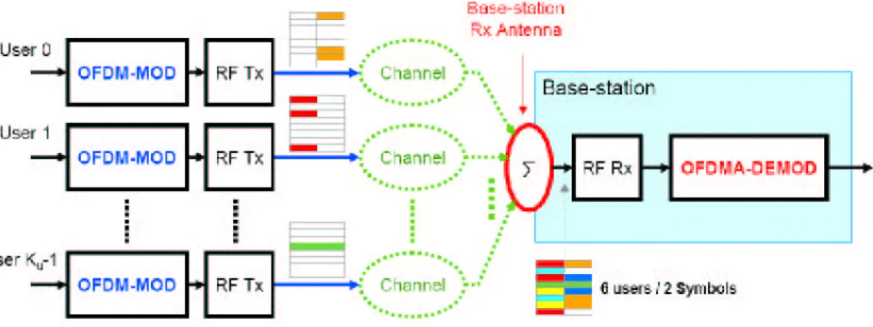
Figure 2.2: Block diagram of an OFDMA system with consecutive subcarriers assign-ment.

sub-carriers to be assigned to different users. For example, sub-carriers 1, 3 and 7 are assigned to user 1 and sub-carriers 2, 5 and 9 to user 2. These groups of sub-carriers are known as sub-channels. Scalable OFDMA allows smaller FFT sizes to improve per-formance (efficiency) for lower bandwidth channels. In essence the principle of OFDMA consists of different users sharing the upstream FFT space, while each transmits one or

Figure 2.3: An OFDMA system with interleaved subcarriers.

more sub-channels. Figures 2.2 and 2.3 show comparison of two systems.

2.2

Basics of OFDMA frame structure

There are three types of OFDMA subcarriers. 1. Data subcarriers for data transmission.

2. Pilot subcarriers for various estimation and synchronization purposes.

3. Null subcarriers for no transmission at all, used for guard bands and DC carriers. Active subcarriers are divided into subsets of subcarriers called subchannels. The sub-carriers forming one subchannel may be, but need not be, adjacent; see Figs. 2.2-2.3.

The pilot allocation is arranged differently in different subcarrier allocation modes. For DL Fully Used Subchannelization (FUSC), the pilot tones are allocated first and then the remaining subcarriers are divided into data subchannels. For DL Partially Used Subchannelization (PUSC) and all UL modes, the set of used subcarriers, that is, data and pilots, is first partitioned into subchannels, and then the pilot subcarriers are allocated from within each subchannel. In FUSC, there is one set of common pilot subcarriers, but in PUSC, each subchannel contains its own set of pilot subcarriers. In

OFDM A symbol number Su bc ar ri er n um be r t FCH Pr ea m bl e D L-M A P U L-M A P DL burst #1 DL burst #2 DL burst #3 DL burst #4 DL burst #5 UL burst #1 UL burst #2 UL burst #3 UL burst #5 UL burst #4 Ranging channel DL _TTG UL Pr ea m bl e FCH D L-M A P RTG

...

Figure 2.4: OFDMA frame structure [2].

a DL, subchannels may be intended for different (groups of) receivers while in UL, Sub-scriber Stations (SS) may be assigned one or more subchannels and several transmitters may transmit simultaneously. The subcarriers forming one subchannel may, but need not be, adjacent. Shown in Figure 2.4 is the OFDM frame structure for Time Division Duplexing (TDD) mode. Each frame is divided into DL and UL subframes separated by Transmit/Receive and Receive/Transmit Transition (TTG and RTG, respectively) gaps. Each DL subframe starts with a preamble followed by the Frame Control Header (FCH), the DL-MAP, and an UL-MAP, respectively.

The FCH contains the DL Frame Prefix (DLFP) to specify the burst profile and the length of the DL-MAP immediately following the FCH. The DLFP is a data struc-ture transmitted at the beginning of each frame and contains information regarding the current frame; it is mapped into the FCH.

2.3

Downlink preamble structure

IEEE standard 802.16e-2005 [3] defines 114 preamble sequences for 32 different base stations; see Figure 2.5. Each BS (base station) divides its coverage area into three seg-ments and transmits a different preamble sequence in each segment. The first symbol

Index ID cell Segment Series to modulate (in hexadecimal format)

0 0 0 0xA6F294537B285E1844677D133E4D53CCB1F182D_{E00489E53E6B6E77065C7EE7D0ADBEAF} 1 1 0 0x668321CBBE7F462E6C2A07E8BBDA2C7F7946D5F_{69E35AC8ACF7D64AB4A33C467001F3B2} 2 2 0 0x1C75D30B2DF72CEC9117A0BD8EAF8E0502461F_{C07456AC906ADE03E9B5AB5E1D3F98C6E} 3 3 0 0x5F9A2E5CA7CC69A5227104FB1CC2262809F3B10_{D0542B9BDFDA4A73A7046096DF0E8D3D} 4 4 0 0x82F8A0AB918138D84BB86224F6C342D81BC8BFE_{791CA9EB54096159D672E91C6E13032F} 5 5 0 0xEE27E59B84CCF15BB1565EF90D478CD2C49EE8_{A70DE368EED7C9420B0C6FFAF9AF035FC} 6 6 0 0xC1DF5AE28D1CA6A8917BCDAF4E73BD93F931C4_{4F93C3F12F0132FB643EFD5885C8B2BCB} 7 7 0 0xFCA36CCCF7F3E0602696DF745A68DB948C57DF_{A9575BEA1F05725C42155898F0A63A248} 8 8 0 0x024B0718DE6474473A08C8B151AED124798F15D1_{FFCCD0DE574C5D2C52A42EEF858DBA5}

....

Figure 2.5: Partial preamble modulation sequences for the 1K FFT mode [3].

of a downlink transmission frame is the preamble. There are three types of preamble carrier-sets, those are defined by the allocations of respective subcarriers. Those sub-carriers are modulated using a boosted BPSK modulation with a specific Pseudo-Noise (PN) code. As mentioned before, the coverage area of a base station is divided into three segments. Each segment uses a preamble composed of a carrier-set out of the three avail-able carrier-sets with the following constraints. For Segment 0, the DC carrier is not

modulated; it shall always be zeroed while the last carrier in Segment 2 shall not be modulated. There will be 172 guard band subcarriers on both sides of the spectrum. The subcarriers associated with a preamble sequence is indexed by

P reambleCarrierSetn = n + 3 · k, (2.1)

where

• P reambleCarrierSetn: specifies all subcarriers allocated to the given (nth)

pream-ble sequence (within a cell).

• n : the number of preamble carrier-set indexed 0, 1, 2. • k : a running index 0, 1, 2 · · · 284.

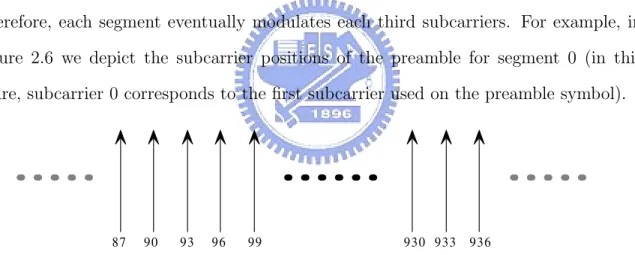
Therefore, each segment eventually modulates each third subcarriers. For example, in Figure 2.6 we depict the subcarrier positions of the preamble for segment 0 (in this figure, subcarrier 0 corresponds to the first subcarrier used on the preamble symbol).

87 90 93 96 99 930 933 936

Figure 2.6: Preamble carrier-set for Segment 0

For 1024 FFT size the PN sequence modulating the preamble carrier-set are defined in [3]. Recall that in case of Segment 0, the preamble symbol has 86 guard band subcarriers on the left and right sides of the spectrum.

2.4

SUI channel model

The SUI (Stanford University Interim) channel models will be used in our study of the performance of various algorithms. This model allows many possible combinations

of parameters to provide a variety of channel descriptions. A set of 6 typical channels is selected for the three typical terrain types. These models are developed for use in simulations, design, development and testing of technologies suitable for broadband wireless applications. Typically scenario for the SUI models are as follows.

• Cells are less than 10 km in radius for a variety of terrain and tree density types. • Under-the-eave/window or rooftop installed directional antennas (2 − 10 m) at the

receiver

• 15 − 40m BTS antennas

• High cell coverage requirement (80 − 90%)

Table 2.1: SUI-1 channel model definition.

SUI-1 channel Tap 1 Tap 2 Tap 3 Units

Delay 0 0.4 0.9 µs Power(omni ant.) 0 -15 -20 dB 90% K Factor(omni ant.) 4 0 0 dB 75% K Factor(omni ant.) 20 0 0 dB Power(300 _{ant.) 0 -21 -32 dB} 90% K Factor(300 _{ant.) 16 0 0 dB} 75% K Factor(300 _{ant.) 72 0 0 dB} Doppler 0.4 0.3 0.5 Hz

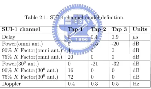
The parameters of the six SUI channels (Figures 2.1 - 5.1), including the propagation scenario that led to this specific set, can be found in the referenced document [4]. The definition of the SUI-3 channel (omni antenna) which is used for our simulations.

2.5

SCM channels

The SCM (spatial channel model) channels are usually used for fixed or mobile wireless applications. It defines three environments (Suburban Macro, Urban Macro,

Table 2.2: SUI-2 channel model definition.

SUI-2 channel Tap 1 Tap 2 Tap 3 Units

Delay 0 0.4 1.1 µs Power(omni ant.) 0 -12 -15 dB 90% K Factor(omni ant.) 2 0 0 dB 75% K Factor(omni ant.) 11 0 0 dB Power(300 _{ant.) 0 -18 -27 dB} 90% K Factor(300 ant.) 8 0 0 dB 75% K Factor(300 _{ant.) 36 0 0 dB} Doppler 0.2 0.15 0.25 Hz

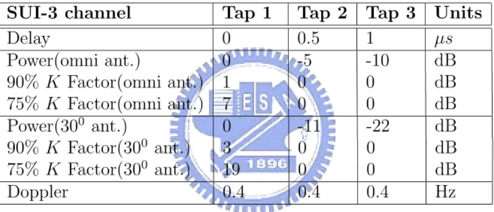
Table 2.3: SUI-3 channel model definition.

SUI-3 channel Tap 1 Tap 2 Tap 3 Units

Delay 0 0.5 1 µs Power(omni ant.) 0 -5 -10 dB 90% K Factor(omni ant.) 1 0 0 dB 75% K Factor(omni ant.) 7 0 0 dB Power(300 _{ant.) 0 -11 -22 dB} 90% K Factor(300 _{ant.) 3 0 0 dB} 75% K Factor(300 _{ant.) 19 0 0 dB} Doppler 0.4 0.4 0.4 Hz

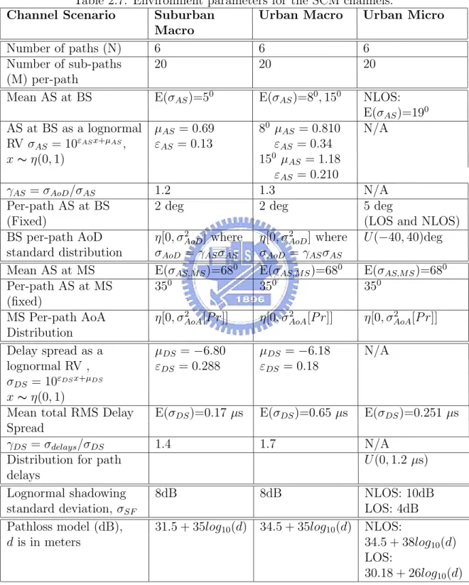
and Urban Micro) where Urban Micro is differentiated in line-of-sight (LOS) and non-LOS (Nnon-LOS) propagation. There is a fixed number of 6 paths in every scenario, each representing a Dirac function in delay domain, but made up of 20 spatially separated sub-paths according to the sum-of-sinusoids method. Path powers, path delays, and angular properties for both sides of the link are modeled as random variables defined through probability density functions and cross-correlations. All parameters, except for fast-fading, are drawn independently in time.

Table 2.7 describes the parameters used in each of the candidate environments. The steps for generating user parameters for urban macrocell and suburban macrocell envi-ronments are as follows. Detailed descriptions and equations are given in [5].

Table 2.4: SUI-4 channel model definition.

SUI-4 channel Tap 1 Tap 2 Tap 3 Units

Delay 0 1.5 4 µs Power(omni ant.) 0 -4 -8 dB 90% K Factor(omni ant.) 0 0 0 dB 75% K Factor(omni ant.) 1 0 0 dB Power(300 _{ant.) 0 -10 -20 dB} 90% K Factor(300 ant.) 1 0 0 dB 75% K Factor(300 _{ant.) 5 0 0 dB} Doppler 0.2 0.15 0.25 Hz

Table 2.5: SUI-5 channel model definition.

SUI-5 channel Tap 1 Tap 2 Tap 3 Units

Delay 0 4 10 µs Power(omni ant.) 0 -5 -10 dB 90% K Factor(omni ant.) 0 0 0 dB 75% K Factor(omni ant.) 0 0 0 dB 50% K Factor(omni ant.) 2 0 0 dB Power(300 _{ant.) 0 -11 -22 dB} 90% K Factor(300 _{ant.) 0 0 0 dB} 75% K Factor(300 _{ant.) 2 0 0 dB} 50% K Factor(300 _{ant.) 7 0 0 dB} Doppler 2 1.5 2.5 Hz

Step 1: Choose either an urban macrocell or suburban macrocell environment. Step 2: Determine various distance and orientation parameters.

Step 3: Determine the DS (delay spread), AS (angle spread), and SF (shadow fading). Step 4: Determine random delays for each of the N multipath components.

Step 5: Determine random average powers for each of the N multipath components. Step 6: Determine AoDs for each of the N multipath components.

Table 2.6: SUI-6 channel model definition.

SUI-6 channel Tap 1 Tap 2 Tap 3 Units

Delay 0 14 20 µs Power(omni ant.) 0 -10 -14 dB 90% K Factor(omni ant.) 0 0 0 dB 75% K Factor(omni ant.) 0 0 0 dB 50% K Factor(omni ant.) 1 0 0 dB Power(300 ant.) 0 -16 -26 dB 90% K Factor(300 _{ant.) 0 0 0 dB} 75% K Factor(300 _{ant.) 2 0 0 dB} 50% K Factor(300 _{ant.) 5 0 0 dB} Doppler 0.4 0.3 0.5 Hz

Step 8: Determine the powers, phases and offset AoDs of the M = 20 sub-paths for each of the N paths at the BS.

Step 9: Determine the AoAs for each of the multipath components.

Step 10: Determine the offset AoAs at the UE of the M = 20 sub-paths for each of the N paths at the MS.

Step 11: Associate the BS and MS paths and sub-paths.

Step 12: Determine the antenna gains of the BS and MS sub-paths as a function of their respective sub-path AoDs and AoAs.

Step 13: Apply the path loss based on the BS to MS distance from Step 2, and the log normal shadow fading determined in Step 3 as bulk parameters to each of the sub-path powers of the channel model.

Table 2.7: Environment parameters for the SCM channels.

Channel Scenario Suburban Urban Macro Urban Micro

Macro

Number of paths (N) 6 6 6

Number of sub-paths 20 20 20

(M) per-path

Mean AS at BS E(σAS)=50 E(σAS)=80, 150 NLOS:

E(σAS)=190 AS at BS as a lognormal µAS = 0.69 80 µAS = 0.810 N/A RV σAS = 10εASx+µAS, εAS = 0.13 εAS = 0.34 x ∼ η(0, 1) 150 _µ AS = 1.18 εAS = 0.210 γAS = σAoD/σAS 1.2 1.3 N/A

Per-path AS at BS 2 deg 2 deg 5 deg

(Fixed) (LOS and NLOS)

BS per-path AoD η[0, σ2

AoD] where η[0, σAoD2 ] where U (−40, 40)deg

standard distribution σAoD = γASσAS σAoD = γASσAS

Mean AS at MS E(σAS,M S)=680 E(σAS,M S)=680 E(σAS,M S)=680

Per-path AS at MS 350 ₃₅0 ₃₅0

(fixed)

MS Per-path AoA η[0, σ2

AoA[P r]] η[0, σAoA2 [P r]] η[0, σ2AoA[P r]]

Distribution

Delay spread as a µDS = −6.80 µDS = −6.18 N/A

lognormal RV , εDS = 0.288 εDS = 0.18

σDS = 10εDSx+µDS

x ∼ η(0, 1)

Mean total RMS Delay E(σDS)=0.17 µs E(σDS)=0.65 µs E(σDS)=0.251 µs

Spread

γDS = σdelays/σDS 1.4 1.7 N/A

Distribution for path U (0, 1.2 µs)

delays

Lognormal shadowing 8dB 8dB NLOS: 10dB

standard deviation, σSF LOS: 4dB

Pathloss model (dB), 31.5 + 35log10(d) 34.5 + 35log10(d) NLOS:

d is in meters 34.5 + 38log10(d)

LOS:

Chapter 3

Frame Detection and Carrier

Frequency Offset Estimation

Link setup refers to the procedure for a mobile unit to be able to “talk” to a base station, which usually involves the following operations. (see Figure 3.1)

• Frame detection (time domain)

• Carrier frequency offset recovery (time or frequency domain) • Segment detection (frequency domain)

• Joint (fine) timing recovery, channel estimation and cell determination

In this chapter, we present solutions for frame detection and carrier frequency offset estimation.

3.1

Frame detection

For the WiMAX system, the preamble lies in the first symbol of the downlink sub-frame after last uplink sub-sub-frame (see Fig. 2.4). BS receive/transmit transition gap (RTG) is a gap between the last sample of the uplink burst and the first sample of the subsequent downlink burst at the antenna port of the base station (BS) in a time division duplex (TDD) transceiver. This gap allows time for the BS to switch from the receive mode to the transmit mode. The length of RTG is usually more than 5µs and

less than 50µs. The first step of cell search is to detect the presence of a downlink signal during the cyclic prefix (CP) period of the first symbol of the downlink sub-frame.

Shown in Fig. 3.2 is the frame and pilot structures of the WiMAX system. As has been defined in Section 2.3, the frequency domain preamble structure results in an almost periodic time domain preamble representation with a period of N/3 (N is FFT size) samples.

To exploit this near-periodic property, we define the autocorrelation functions C1[n] = n+N/3−1_X i=n r∗[i]r[i + N/3] C2[n] = n+N/3−1_X i=n r∗[i]r[i + 2N/3] C3[n] = n+N/3−1_X i=n r∗[i + N/3]r[i + 2N/3] (3.1)

where {r[i]} is the received time domain sample sequence. The corresponding normalized versions are defined as

C1 nor[n] = ¯ ¯ ¯ ¯ ¯ Pn+N/3−1 i=n r∗[i]r[i + N/3] Pn+N/3−1 i=n r∗[i + N/3]r[i + N/3] ¯ ¯ ¯ ¯ ¯, (3.2) C2 nor[n] = ¯ ¯ ¯ ¯ ¯ Pn+N/3−1 i=n r∗[i]r[i + 2N/3] Pn+N/3−1 i=n r∗[i + 2N/3]r[i + 2N/3] ¯ ¯ ¯ ¯ ¯, (3.3) C3 nor[n] = ¯ ¯ ¯ ¯ ¯ Pn+N/3−1 i=n r∗[i + N/3]r[i + 2N/3] Pn+N/3−1 i=n r∗[i + 2N/3]r[i + 2N/3] ¯ ¯ ¯ ¯ ¯, (3.4)

To make the most of all the correlation information, we further define the normalized total correlation function

C[n] = C1 nor[n] + C2 nor[n] + C3 nor[n] (3.5)

Fig. 3.3 depicts the normalized total correlation C[n] as a function of the initial sampling time instant. As can be seen from this figure, C[n] stars to increase slowly at n = N/3,

i.e., the starting instant of the pilot sequence. The maximum correlation value is reached when n is equal to the cyclic prefix duration. After that C[n] begins to decrease linearly. The peak of the autocorrelation C[n] coincides with the “arrival time” of the incoming pilot sequence. As C[n] is a relatively smooth function, its first derivative (difference) also gives useful indication of the arrival of a new downlink frame with the peak occurs at ∆C[n] = C[n] − C[n − 1] ≈ 0. Hence, the amplitude and slope variations of the C[n] can be used to detect the presence of a preamble symbol (sequence). However, the presence of noise and interference makes the correct detection of the initial pilot position (i.e., coarse timing) very difficult. Instead of searching for the peak correlation or the zero first-order difference position, a more robust scheme for coarse timing is the moving window peak detector. We define the moving average of size 2l = lCP (the cyclic prefix

length) Sc[k] = 1 2l (2k+1)l_X n=(2k−1)l C[n] (3.6)

Then the peak correlation occurs at n = 2kl where k is such that

Sc[k − 1] < Sc[k] and Sc[k] > Sc[k + 1] (3.7)

If the condition described in equation 3.7 holds, the frame timing acquisition is given by

etf rame = 2kl (3.8)

Using the following recursive relations:

C1[n + 1] = C1[n] + r∗[n + N/3]r[n + 2N/3] − r∗[n]r[n + N/3]

C2[n + 1] = C2[n] + r∗[n + N/3]r[n + 3N/3] − r∗[n]r[n + 2N/3]

C3[n + 1] = C3[n] + r∗[n + 2N/3]r[n + 3N/3] − r∗[n + N/3]r[n + 2N/3]

C[n + 1] = C[n] + r∗[n + N/3]r[n + 3N/3] + r∗[n + 2N/3]r[n + 3N/3]

− r∗[n]r[n + N/3] − r∗[n]r[n + 2N/3] (3.9)

identities indicate that the MA peak detector needs about (N + lCP) × p bits memory

where p is the number of bits per sample.

3.2

Carrier frequency offset estimation

Carrier frequency offset (CFO) is often caused by the frequency synthesizer insta-bilities, the relative movement between the transmitter and the receiver, and the time-varying nature of the transmission media. CFO is especially problematic in multi-carrier (e.g., OFDM) system as compared to single carrier system. Our CFO estimation algo-rithm exploits the repetitive property of the preamble symbol. Fig. 3.4 shows that the

received time domain pilot sequence has three L = N/3 periods and F1 denotes the

cross-correlation between samples in the first period and the conjugate of those in the second period. F1 = L−1 X n=0 r[n]r∗[n + L] = L−1 X n=0 x[n]ej2πεn/N(x[n + L]ej2πε(n+L)/N)∗ = L−1 X n=0 x[n]x∗[n + L]ej2πεn/Ne−j2πε(n+L)/N = e−j2πεL/N L−1 X n=0 x[n]x∗[n + L] (3.10)

where ε is the CFO. Similarly, F2 is the cross-correlation between the samples in the

first period and those in the conjugate of the third period. F2 = L−1 X n=0 r[n]r∗[n + 2L] = e−j2πε2L/N L−1 X n=0 x[n]x∗[n + 2L] (3.11)

In the absence of noise and CFO, the phases associated with a pair of samples two periods apart, x[n], x[n + 2L], should be the same so that the above summation is a real number. Hence, ε can be estimated either by F1 or by F2. However, the phase of two

preamble sequence belongs to. For example, for Segment 0, we have x[n]x∗[n + L] = Ã_n−1 X i=0 X[i]ej2πniN ! Ã_n−1 X k=0 X∗[k]e−j2π(n+L)kN ! = n−1 X k=0 X[k]X∗[k]e−j2πLkN + C[k] ∼₌ N −1 3 X k0₌₀ e−j2π(3k0+2)3 + C[k] = N −1 3 X k0₌₀ e−j4π3 + C[k] (3.12) where C[k] = N −1_X i=0 N −1_X k=0,k6=i X[i]ej2πniN · ³ X∗[k]e−j2π(n+L)kN ´ = N −1_X i=0 N −1_X k=0,k6=i

X[i]X∗[k]ej2πn(i−k)N e−j 2πkL

N (3.13)

whose average is approximately zero, E (_{N −1} X i=0 N −1_X k=0,k6=1

X[i]X∗[k]ej2πn(i−k)N e−j2πkLN

)

∼_{= 0 (3.14)}

Therefore

arg (x[n]x∗[n + L]) ∼= −4π/3 = 2π/3 (3.15)

arg(x) denotes the principal argument (angle) of the complex number x. Similarly, it can be shown that the phase of x[n]x∗_{[n + 2L] is complementary to that of x[n]x}∗_{[n + L].}

For Segment 0, x[n]x∗[n + 2L] = Ã_n−1 X i=0 X[i]ej2πniN ! Ã_n−1 X k=0 X∗[k]e−j2π(n+2L)kN ! = n−1 X k=0 X[k]X∗[k]e−j2π2LkN + C[k] ∼ = N −1 3 X k0₌₀ e−j4π(3k0+2)3 + C[k] = N −1 3 X k0₌₀ e−j8π3 + C[k] (3.16)

Therefore,

arg (x[n]x∗[n + 2L]) ∼= −8π/3 = −2π/3

Fig. 3.5 shows some typical values of the complex product y[n] = x[n]x∗_{[n + L], n =}

0, 1, 2, · · · , (L − 1). The phase of the summation (time average) 1 L L−1 X n=0 x[n]x∗_{[n + L]}

is obviously 2π/3, which confirms our previous derivation. As the phases of PL−1_n=0x[n]x∗_{[n + L] and} PL−1

n=0x[n]x∗[n + 2L] tend to cancel each

other, the phase of F is caused by CFO only. Consequently, the fractional part of the CFO can be derived from F , i.e., the product of F1 and F2

F = F1· F2 = e−j2πε Ã_L−1 X n=0 x[n]x∗[n + L] ! Ã_L−1 X n=0 x[n]x∗[n + 2L] ! (3.17) via b ε = −arg(F ) 2π

where it is assumed that ² < ±0.5 subcarrier spacings is the true CFO and _bε is its estimate. Fig. 3.6 shows the mean squared error (MSE) performance of the above CFO algorithm in an AWGN channel.

The computational complexity for this CFO estimate includes 2N/3 complex multi-plications, 2N/3 complex additions and p × (N + lCP) bits storage.

Frame detection C FO estimation segment decision frequency correlation FFT verification IFFT Yes No group repartition fine timing recovery FFT noncoherent FD_MF bank joint channel and sequence estimation peak detection

OFDM A symbol number Su bc ar ri er n um be r t FCH Pr ea m bl e D L-M A P U L-M A P DL burst #1 DL burst #2 DL burst #3 DL burst #4 DL burst #5 UL burst #1 UL burst #2 UL burst #3 UL burst #5 UL burst #4 Ranging channel DL _TTG UL Pr ea m bl e FCH D L-M A P RTG

...

Figure 3.2: WiMAX downlink frame structure and the corresponding time domain preamble sequence.

0 200 400 600 800 1000 1200 0.4 0.6 0.8 1 1.2 1.4 1.6 1.8 2 n (sampling time)

Normalized total correlation

Figure 3.3: Normalized total correlation as a function of the initial sampling instant n. The down-link frame arrives at n = 500. The peak correlation occurs at n = CP duration; N = 1024 subcarriers , lcp = 64 bits.

cp

L

F

cp

L

F

CP

N/3

N/3

N/3

L

Figure 3.4: Time domain preamble (pilot) symbol exhibits a repetitive structure.

CP N/3 N/3 N/3

conjugate

conjugate

−1 −0.8 −0.6 −0.4 −0.2 0 0.2 0.4 0.6 0.8 1 x 10−3 −8 −6 −4 −2 0 2 4 6 8x 10 −4

Real part of y[n]

Image part of y[n]

Figure 3.5: Some typical values of the complex product y[n] = x[n]x∗_{[n + L] for n :}

8 10 12 14 16 18 10−6

10−5 10−4

SNR (dB)

Mean Square Error

Figure 3.6: The MSE performance of the proposed CFO estimator in an AWGN channel; N = 1024 subcarriers and the cyclic prefix is 64-bit long.)

Chapter 4

Segment Decision and Cell

Acquisition

After frame detection (coarse timing estimate) and CFO compensation, the received sequence will be transformed into frequency domain via Fast Fourier Transform (FFT). From the frequency domain samples we have to decide to which segment the received sequence belongs. The segment decision can be performed by utilizing the segment-dependent frequency domain pilot structure (see Fig. 4.1). When a correct segment decision is reached, the number of candidate pilot sequences reduces from 114 to 38. Cell is acquired when the ambiguity about the remaining 38 candidate sequences is resolved. As will be shown, this final step of the cell search procedure also yields fine timing and channel estimates. In fact, these estimates are obtained in conjunction with sequence acquisition.

In Section 4.4, we suggest another approach for joint channel estimation and cell search without the need of the fine timing information, which is obtained after cell sequence is synchronized.

4.1

Segment decision

The preamble structure is defined in Section 2.3 and Fig. 4.1 shows their frequency domain allocations for different segments. It is clear that pilot sequences in different segments are orthogonal in the sense that for pilot sequences Xi[k], Xj[k] in the ith and

jth segments always satisfy

Xi[k]Xj∗[k] = 0, ∀ k, and i 6= j

This orthogonality property suggests that segment decision should be made by subband energy detection, counting energy content in the subcarrier locations associated with a segment. Assuming perfect CFO compensation and a residual timing offset of ∆t, the

...

...

...

guard interval guard interval

87 90 93 930 933 936

segment 0

...

...

...

guard interval guard interval

88 91 94 931 934 937

segment 1

...

...

...

guard interval guard interval

89 92 95 932 935 938

segment 2

Figure 4.1: Sub-carriers allocations for different segments.

received baseband sample x[n] = ˜x[n−∆t] has a frequency domain representation X[k] = e−j2πkN ∆tX[k], where { ˜˜ X[k]} is the discrete Fourier Transform of the zero-timing error

sequence {x[n]}. Since the magnitude of frequency domain representation is independent of the timing error, segment decision can be made without accurate timing information. We say that the received sequence belongs to ith segment if Dseg(i) has the maximum

value amongst the three segment energy detectors {Dseg(l), l = 0, 1, 2}, i.e.,

ˆi = arg max

where Dseg(1) = 312 X k=29 |X[3k]|2 Dseg(2) = 312 X k=29 |X[3k + 1]|2 Dseg(0) = 312 X k=29 |X[3k + 2]|2 (4.2)

The algorithmic complexity for segment decision includes 2N real multiplications, N real additions and (N + lCP) × p bits memory.

4.2

Group association: joint cell search and timing

estimation

After a segmentation decision is made, the number of possible preamble sequences is reduced to 38. Invoking the fact that the cross correlations between any pair of preamble sequences are very low, we partition 38 preamble sequences to M groups and form a sum-sequence for each group. For example, we can partition 38 preamble sequences into M = 6 groups and form 6 sum-sequences with the components of these sequences given by P1[n] = 6 X i=1 pi[n], P2[n] = 12 X i=7 pi[n], P3[n] = 18 X i=13 pi[n], P4[n] = 24 X i=19 pi[n], P5[n] = 31 X i=25 pi[n], P6[n] = 38 X i=32 pi[n], (4.3)

where pi[n] is the nth component of the ith preamble sequence. The 1 × 1024 vector

Pk = (Pk[0], Pk[1], · · · Pk[1023]) is the kth sum-sequence.

Let F−1_{{·} denote the inverse Fourier transform and ¯ represent Kronecker}

(com-ponentwise) product. Then

gives the correlation magnitude between the received sample sequence and the ith sum-sequence at various lags (timing epochs). If the received sum-sequence belongs to the ith group and ∆n is the coarse timing error, Zi[n] will have peak values at n = N/3 − ∆n,

n = 2N/3 − ∆n and n = N − ∆n while the other positions contain noise only and give low correlation magnitudes.

0 200 400 600 800 1000 1200 0 0.05 0.1 0.15 0.2 0.25 0.3 0.35 0.4 n (timing lag) Correlation magnitude

Figure 4.2: The correlation magnitude Z1[n] between the received sample sequence and

the first sum-sequence at various lags. Subband energy detector output is maximized at the true locations; N = 1024 subcarriers and lcp = 64 bits.

As one can see from Figures 4.2 and 4.3, if the true transmitted preamble sequence belongs to the 1th group, Z1[n] will have large peak values and Zk[n] for k 6= 1 will be

much smaller. Hence one can easily determine to which segment the received preamble sequence belongs.

0 200 400 600 800 1000 1200 0 0.05 0.1 0.15 0.2 0.25 0.3 0.35 0.4 n (timing lag) Correlation magnitude

Figure 4.3: The correlation magnitude Z2[n] between the received sample sequence and

the 2nd sum-sequence at various lags; N = 1024 subcarriers, lcp = 64 bits.

F−1_{P

i[k]} and the received preamble sequence is three-period long, Zi[n] will have

three equally-spaced peaks. Define Wi[n] = Zi[n] + Zi · n + N 3 ¸ + Zi · n + 2N 3 ¸ n ∈ D = {0, 1, 2, · · · 340}. (4.5) and Wmax = max n∈D Wi[n]

kmax = arg max

n∈D Wi[n] W_max0 = max n∈D\kmaxWi[n] r = Wmax W0 max (4.6)

Frame detection C FO estimation segment decision frequency correlation FFT verification IFFT Yes No group repartition fine timing recovery FFT noncoherent FD_MF bank joint channel and sequence estimation peak detection

Table 4.1: Peak subband energy detector output ratio behavior as a function of SNR (dB); N = 1024 subcarriers, lcp= 64 bits, T = correct group identification, F = incorrect

group identification. SNR = 8 SNR = 10 SNR = 12 r (T) 1.6105 1.621 1.6152 r (F) 1.0149 1.0018 1.0111 SNR = 14 SNR = 16 SNR = 18 r (T) 1.6358 1.6332 1.6181 r (F) 1.0119 1.0018 1.0363

Wmax is the largest value among Wi[n], Wmax0 is the second largest value and r is the

ratio between the largest and the second largest values of Wi[n].

Table 4.1 list some typical values for r at different SNRs. It is obvious the largest-to-the-second-largest ratio r is insensitive to the SNR variation. Hence it is a reliable indicator for a group association decision (GAD), i.e., it can be used to if the decision about the incoming sequence belongs to a given group is a reliable one.

When a GAD is deemed unreliable because r < γ = 1.25, a new group partition is called for. We choose three groups which have the largest peak values and divid-ing the corresponddivid-ing member sequences into four groups. Followdivid-ing a similar pro-cedure we obtain the new sum-sequences {P11, P12, P13, P14}, compute the correlations

{Z11[n], Z12[n], Z13[n], Z14[n]} and the corresponding ratio r again.

When the ratio r exceeds the threshold γ, the cell identification is likely to be correct and the timing information can be deduced from the positions of the peaks. If one decide the received preamble sequence belongs to ith group, the fine frame timing will be obtained by ˆ t = arg max n∈D ½ Zki[n] + Zki · n + N 3 ¸ + Zki · n + 2N 3 ¸¾ c ∆n = ˆt − µ N 3 − lcp ¶ (4.7) where lcpis length of CP (cyclic prefix). Figs. 4.5 and 4.6 show false cell detection

8 10 12 14 16 18 1E-4

1E-3 0.01

False Cell Detection Prob.

Average SNR (dB)

without verification with verification

Figure 4.5: Probability of false cell detection in a SUI-3 channel.

0 2 4 6 8

1E-3 0.01 0.1

False Cell Detection Prob.

Average SNR (dB)

without verification with verification

easily see that the addition of a verification mode brings about significant improvement. The computational complexity for this step is 6N log2N +2N complex multiplications

and (N + lCP + 6N ) × p bits memory at least.

4.3

Joint channel estimation and sequence

identifi-cation

After obtaining fine frame timing and the sequence group association, the number of candidate sequences is reduced to ≤ 7. This ambiguity can be resolved by using a bank of frequency domain noncoherent correlators (matched filters), each matches to a given sequence. Let ˜x[n] be the received time domain sequence with perfect CFO com-pensation, Pi = (Pi[0], Pi[1], · · · , Pi[N − 1]), ˜X[k] =DFT{˜x[n]}, and ˆP be the estimated

preamble sequence. Then ˆ P = max Pi ¯ ¯ ¯ ¯ ¯ N −1 X k=0 ˜ X[k]Pi[k] ¯ ¯ ¯ ¯ ¯ (4.8)

This approach is referred to as the noncoherent frequency domain matched filter bank (FD-MFB) algorithm. A more reliable approach is through joint channel estimation and cell identification. Note that the received frequency domain sample is given by

˜

X[k] = H[k]Pi[k] + W [k], k = 0, 1, · · · , N − 1 (4.9)

Hk is the channel response at the kth subcarrier, and Nk is the corresponding white

Gaussian noise (WGN) with variance N0

2 . Channel estimation in an OFDM system can

be based on least squares (LS) criterion. The LS estimator, which does not require any channel information, minimizes the squared error e = ||Y − ˆHX||2 _{= (Y − ˆHX)}H_{(Y −}

ˆ

HX), where (·)H _{denotes the conjugate transpose operation. It is shown that the}

pilot-assisted LS estimator of H is given by b

HLS = X−1Y

where X[k] are pilot symbols. If the candidate preamble sequences are {P1, P2, P3, P4,

P5, P6}, the corresponding LS channel estimates are given by

ˆ H1[k] = ˜ X[k] P1[k] ˆ H2[k] = ˜ X[k] P2[k] ˆ H3[k] = ˜ X[k] P3[k] ˆ H4[k] = ˜ X[k] P4[k] ˆ H5[k] = ˜ X[k] P5[k] ˆ H6[k] = ˜ X[k] P6[k] , k = 0, 1, 2, · · · , N − 1 (4.11) In order to determine which one is the most accurate channel response, we use the assumption that the true channel response is smooth function so that the magnitude of the correlation function

RH[τ ] = N −2 X k=0 ˆ Hi[k] ˆHi∗[k + τ ] (4.12)

is a decreasing function of τ when |τ | is small. Based on such an assumption, a correct pilot sequence will give a smooth channel estimate but an incorrect one leads to random and non-smooth estimate. Therefore we propose the following joint channel and sequence estimate (JCSE) algorithm.

ˆj = arg max i ¯ ¯ ¯ ¯ ¯ N −2_X k=0 ˆ Hi[k] ˆHi∗[k + 1] ¯ ¯ ¯ ¯ ¯ b P = Pˆj b HLS = bP−1Y (4.13)

The noncoherent FD-MFB approach needs only 6 × N/3 complex additions since Pi[k]

are ±1-valued. Similarly, the JCSE approach for cell identification needs 6 × N/3 com-plex additions and N/3 comcom-plex multiplications for computing channel autocorrelation function.

False cell (sequence) identification (detection) probability performance of the above two methods is shown in Fig. 4.9. The latter approach which performs joint channel estimation and sequence identification, taking into account the channel smoothness, is a much better solution, especially if SNR is high.

0 10 20 30 40 50 60 70 80 90 100 −1.2 −1 −0.8 −0.6 −0.4 −0.2 0 0.2 0.4 subcarrier index(k) H_true H_LS

Figure 4.7: Channel estimate by a correct preamble sequence.

4.4

Cell search without group association

The group association stage reduces the sequence (cell) identification ambiguity and provides fine frame timing simultaneously. An alternative approach is to bypass this stage and go directly for cell identification. In this case a joint cell search and channel estimation without fine timing is needed. We refer to this approach as the direct cell identification method. Let ∆t be the timing offset.

b Hi[k] = ˜ X[k] Pi[k] = H[k]e−j2πkN ∆t+ W0 i[k] ˆj = arg max i ¯ ¯ ¯ ¯ ¯ N −2_X k=0 ˆ Hi[k] ˆHi∗[k + 1] ¯ ¯ ¯ ¯ ¯ = arg max i ¯ ¯ ¯ ¯ ¯ N −2_X k=0 ˜ X[k] ˜X∗_{[k + 1]} Pi[k]Pi∗[k + 1] ¯ ¯ ¯ ¯ ¯= arg maxi ¯ ¯ ¯ ¯ ¯ N −2_X k=0 H[k]H∗[k + 1]ej2πN∆t ¯ ¯ ¯ ¯ ¯ b P = Pˆ_j b Hˆj = bP−1Y (4.14)

0 10 20 30 40 50 60 70 80 90 100 −1.5 −1 −0.5 0 0.5 1 subcarrier index(k) H_true H_LS

Figure 4.8: Channel estimate by an incorrect preamble sequence.

where W0

i[k] = W [k]/Pi[k] and the right-most part of the third equation has ignore the

noise terms and is intended to show that the magnitude of the LS-estimated channel correlation is independent of coarse timing error ∆t. The complexity of this method is lower than that mentioned in previous sections. It requires only N/3 complex multi-plications and 38 × N/3 complex additions. The algorithms of Fig. 4.4 need at least 6N log₂N + 2N + N/3 complex multiplications. The false detection probability perfor-mance of the two approaches are compared in Figures 5.2 (for an SUI-3 channel) and 5.3 (for an SCM channel). Since the direct cell identification approach results in superior performance, the group association stage seems to be a redundant intermediate step and should be avoided.

8 10 12 14 16 1E-3

0.01 0.1

False Cell Detection Prob.

Average SNR (dB)

Noncoherent FD-MFB algorithm JCSE algorithm

Figure 4.9: Performances comparison between the noncoherent frequency domain matched filter bank (FDMFB) approach and the joint channel/sequence estimation (JCSE) method in a SUI-3 channel.

Frame detection C FO estimation segment decision FFT joint channel and sequence estimation

8 10 12 14 16 1E-4

1E-3 0.01

False Cell Detection Prob.

Average SNR (dB)

indirect(group association) cell identification

direct cell identification

Figure 4.11: Performance of the direct cell identification approach in an SUI-3 channel (1024 subcarriers, 64-bit long CP).

0 1 2 3 4 5 6 1E-5 1E-4 1E-3 0.01 0.1

False Cell Detection Prob.

Average SNR (dB)

indirect(group association) cell identification

direct cell identification

Figure 4.12: Performance of the direct cell identification approach in an SCM channel (1024 subcarriers, 64-bit CP).

Chapter 5

Cell Search in the Presence of Large

CFO

The discussion so far assumes a CFO that is less than half a subcarrier spacing. When this assumption is not valid, i.e., if CFO is greater than one subcarrier spacing, the proposed solution (at least the segmentation part) can no longer work since the frequency domain characteristic of the pilot sequences is of no use. A straightforward solution is apply the direct cell search procedure to the 114 pilot sequences. The first two steps–frame detection and fractional CFO estimation–are the same as any one of previous algorithms. For simplicity we assume that the fractional CFO has been compensated for perfectly. Neglecting the noise contribution for the time being, the received sequence with an integer CFO ` is given by

e X[k] = H[k]X[k + `]e−j2πkN ∆t (5.1) Let ˆHi[k, l] = eX[k]/Pi[k + l] {ˆj, ˆ`} = arg max i, l N −2_X k=0 ˆ Hi[k, l] ˆHi∗[k + 1, l] = max i, l N −2_X k=0 H[k, l]H∗[k + 1, l]ej2πN∆t (5.2) ˆ P = Pˆ_j (5.3)

The overall procedure is shown in Fig.5.1 . The associated computational complexity includes N complex multiplications and at least 3×(114×N ) complex additions. Figures

5.2 (in an SUI-3 channel) and 5.3(in an SCM channel) depict the performance of the proposed direct search without segmentation (DS-WOS) method when (i) there is an integer CFO and (ii) only a fractional CFO is present. Table 5.1 compares the complexity requirements for the previous direct search with segmentation (DS-WS) approach and the DS-WOS approach.

Table 5.1: Complexity parison for the DS-WS and DS-WOS algorithms

Complexity DS-WS DS-WOS

complex addition 38 × N/3 + N 3 × (114 × N/3) (at least)

complex multiplication N/3 N memory (sample) (N + lcp) × p (N + lcp) × p Frame detection fractional C FO estimation FFT direct search without segmentation

8 9 10 11 12 13 14 1E-4

1E-3 0.01

False Cell Detection Prob.

Average SNR (dB)

DS-WS DS-WOS

Figure 5.2: False cell detection probability of the DS-WOS approach in the presence of integer CFO; SUI-3 channel, 1024 subcarriers, 64-bit CP.

0 1 2 3 4 5 6

1E-5 1E-4 1E-3

Flase Cell Detection Prob.

Average SNR (dB)

DS-WS DS-WOS

Figure 5.3: False cell detection probability performance of the DS-WOS approach in the presence of integer CFO; SCM channel, 1024 subcarriers, 64-bit CP.

Chapter 6

Conclusion

We present cell search (sequence identification) algorithms for the IEEE 802.16e standard (WiMAX). Our solutions call for coarse acquisition of frame timing and fractional CFO be carried out in time domain, exploiting the near-periodic pilot structure. These two operations are followed by joint fine timing recovery, cell determination and channel estimation. Two different approaches are proposed. The first one requires a group association stage while the second one–called direct cell search with segmentation–can do without it, yielding a less complex choice. The segmentation algorithm is no longer useful when an integer CFO is present. We therefore modify the cell search procedure, bypassing the segmentation stage (but still keeping the frame detection and fraction CFO estimation stages) and adding a integer CFO search operation. This approach calls for more than 9 times additional operations. Computer simulation results show that the proposed schemes do provide outstanding performance and enable a fast cell search and initial link setup for WiMAX system in multipath fading channels.

Bibliography

[1] Koffman and Roman, ”Broadband wireless access solutions based on OFDM access in IEEE 802.16”, IEEE Comm. Magazine, pp 94-103, Apr. 2002

[2] H. Yaghoobi and Intel Communications Group,”Scalable OFDMA physical layer in IEEE 802.16 wirelessMAN”, Intel Technology Journal, vol. 8, 2004

[3] ”IEEE Standard for Local and metropolitan area networks”,IEEE Std 802.16e, Dec. 2005

[4] ”Channel model for fixed wireless applications” , IEEE 802.16.3c-01/29r4, July 2001.

[5] ”Spatial channel model for Multiple Input Multiple Output (MIMO) simulations”,

3GPP TR 25.996 V6.1.0, Sep. 2003.

[6] H. Lim and D.S. Kwon,”Initial synchronization for WiBro”, IEEE CNF, pp. 284-288, Oct. 2005.

誌謝

作者簡歷

Graduate Course:

4. Digital Signal Processing

5. Detection and Estimation Theory 6. Adaptive Signal Processing

7. Special Topics in Digital Signal Processing 8. Special Topics in Communication Systems