主動土壓力模型擋土牆設計與建造

國立交通大學

土木工程學系碩士班

碩士論文

主動土壓力模型擋土牆之設計與建造

Design and Construction of

NCTU K

Model Retaining Wall

研 究 生：侯鵬暉

指導教授：方永壽 博士

中華民國九十五年九月

ii

主動土壓力模型擋土牆之設計與建造

Design and Construction of NCTU K

Model Retaining Wall

研究生：侯鵬暉 Student:

Peng-Hui

Hou

指導教授：方永壽 博士 Advisor:

Dr.

Yung-Show

Fang

國立交通大學

土木工程學系碩士班

碩士論文

A Thesis

Submitted to Department of Civil Engineering

College of Engineering

National Chiao Tung University

In Partial Fulfillment of the Requirements

for the Degree of

Master

in

Civil Engineering

September 2006

Hsinchu, Taiwan, Republic of China

中華民國九十五年九月

i

主動土壓力模型擋土牆之設計與建造

學生：侯鵬暉

指導教授：方永壽 博士

國立交通大學土木工程學系碩士班

Abstract (in Chinese)

本研究探討夯實土壓力作用於垂直擋土牆上主動土壓力之影響。本研究使 用重新設計建造之 NCTU KA 模型檔土牆模型設備，探討平移模式牆位移所造 成之土壓力變化，根據實驗結果，得到以下結論： 1. 由夯實造成之土壤壓力，隨著牆面外移而迅速消散。達到主動土壓力所 需之牆移動量 S/H 為 0.0010。 2. 主動土壓力分布在從牆頂往下起算牆高三分之一內，側向土壓力略高於 Coulomb 理論解，於牆高中間三分之一的範圍，與 Coulomb 理論解相 近，牆底往上起算三分之一牆高內，則略低於 Coulomb 理論解。 3. 水平土壓力係數 Kh 隨著牆位移增加而下降並達到穩定。主動狀態於牆 位移約 S/H 為 0.001 時發生。

4. 實驗 Ka,h 之數據，與 Coulomb 及 Rankine 的預測相符。

5. 主動合力位置為距牆底 0.55H 處。

6. 由夯實所得之主動係數 Ka,h 值，與 Coulomb 和 Rankine 的預測相符。

7. 主 動 土 壓 力 所 造 成 的 破 壞 面 ， 於 土 壤 表 面 出 現 的 分 裂 位 置 ， 則 與 Rankine 之預測位置相符。

ii

Design and Construction of NCTU K

Model Retaining Wall

Student: Peng-Hui Hou

Advisor: Dr. Yung-Show Fang

Department of Civil Engineering

National Chiao Tung University

Abstract

This paper presents experimental data of earth pressure acting against a vertical rigid wall, which moved outward a mass of dry sand with a stress-free horizontal surface under translation wall-movement. To investigate the variation of earth pressure induced by compaction and active wall movement, the instrumented KA

model retaining wall facility was designed and constructed at National Chiao Tung University. Based on experimental data, the following conclusions can be drawn.

1. The earth pressure induced by compaction vanished rapidly with the active wall movement. An active state of stress is reached at the wall movement of S/H = 0.0010.

2. The distribution of active earth pressure is slightly higher than Coulomb’s solution at the upper one-third of wall height, approximately in agreement with Coulomb’s solution in the middle one-third, and lower than

Coulomb’s solution at the lower one-third of wall surface. Stresses that was locked-in the soil element has been released with the lateral extension of the active soil wedge.

iii

3. The horizontal earth presure coefficient Kh decreases with increasing wall

movement and finally a constant total thrust is reached. The active condition occurred at the wall movement of approximately S/H= 0.001. 4. The experimental Ka,h values are in good agreement with Coulomb and

Rankine’s prediction.

5. The active thrust is located at about 0.55H above the base of the wall. 6. The active coefficient K_a,h values obtained with compacted dense sand

from this study are in fairly good agreement with Coulomb and Rankine’s prediction.

7. The Rankine theory is suitable to predict the location of surface crack for active failure.

iv

Table of Contents

Abstract (in Chinese)... i

Abstract... ii

Table of Contents ... iv

List of Tables... vii

List of Figures ... viii

List of Symbols ... xiv

Chapter 1 Introduction ... 1

1.1 Objective of Study ... 2

1.2 Research Outline... 3

1.3 Organization of Thesis... 4

Chapter 2 Literature Review... 5

2.1 Active Earth Pressure Theories ... 5

2.1.1 The Coulomb Theory ... 5

2.1.2 The Rankine Theory... 7

2.1.3 The Terzaghi Theory ... 8

2.1.4 Comparison of Active Earth Pressure Coefficient Ka...10

2.2 Laboratory Model Retaining Wall Tests for Active State ...11

2.2.1 Model by Terzaghi ...11

2.2.2 Model by Mackey and Kirk...12

2.2.3 Model by Bros ...12

v

2.2.5 Model by Fang and Ishibashi ...14

2.2.6 Model Study by Fang et al. ...16

2.3 Effects of Soil Compaction in Earth Pressure ...17

2.3.1 Study of Peck and Mesri ...17

2.3.2 Study of Chen ...19

Chapter 3 Design of NCTU KA Model Retaining Wall Facility...21

3.1 Design Motivation ...22

3.1.1 Large-scale model wall ...22

3.1.2 Wall driven by servo motors...22

3.1.3 Large wall displacement...23

3.2 Types of Experiments ...23

3.3 NCTU KA Model Retaining Wall Facility...24

3.3.1 Soil Bin...25

3.3.2 Model Wall ...27

3.3.3 Driving System ...34

3.3.4 Data Acquisition System ...36

Chapter 4 Backfill and Interface Characteristics...37

4.1 Backfill Properties ...37

4.1.1 Characteristics of Backfill...37

4.1.2 Air Pluviation of Backfill ...38

4.1.3 Compaction of Backfill ...39

vi

4.2 Interface Friction ...41

4.2.1 Side Wall Friction ...41

4.2.2 Model Wall Friction ...41

Chapter 5 Experimental Results ...43

5.1 Earth pressure due to compaction ...43

5.2 Wall movement required to achieve active state...44

5.3 Experimental results ...44

5.3.1 Distribution of horizontal earth pressure ...44

5.3.2 Variation of horizontal earth pressure coefficient ...45

5.3.3 Location of soil-thrust...45

5.3.4 Active earth pressure coefficient ...46

5.4 Surface crack ...46

5.5 Mechanism of stress reduction of compaction-induced pressure...47

Chapter 6 Conclusions...49

References...51

vii

List of Tables

Table 3.1. Wall displacements required to reach active state ...56

Table 4.1. Properties of Ottawa sand ...57

Table.5.1 Active wall movement at the end of compaction...58

viii

List of Figures

Fig. 1.1 Common uses of retaining walls (after Fang, 1983)...59

Fig. 1.2 Earth pressure under active wall movement ...60

Fig. 2.1 Coulomb’s theory of active earth pressure ...61

Fig. 2.2 Determination of Coulomb’s active earth pressure ...62

Fig. 2.3 Rankine’s theory of active earth pressure...63

Fig. 2.4 Failure surface in soil by Terzaghi’s log-spiral method...64

Fig. 2.5 Evaluation of active earth pressure by trial wedge method ...65

Fig. 2.6 Stability of soil mass abd1f1...66

Fig. 2.7 Active earth pressure determination with Terzaghi’s log-spiral failure surfaces...67

Fig. 2.8 Comparison of coefficient of horizontal component of active pressure for various theories (after Morgenstern and Eisenstein, 1970)...68

Fig. 2.9 MIT model retaining wall ( after Terzaghi, 1932 ) ...69

Fig. 2.10 Earth pressure coefficient K affected by yield of wall (after Terzaghi, 1934)...70

Fig. 2.11 Height of center of pressure in relation to yield of wall (after Terzaghi, 1934)...71

Fig. 2.12 University of Manchester model retaining wall (after Mackey and Kirk, 1967)...72

Fig. 2.13 Earth pressure with wall movement ( after Mackey and Kirk, 1967)...73

Fig. 2.14 Failure surfaces ( after Mackey and Kirk, 1967) ...74

Fig. 2.15 College of Agriculture model retaining wall (after Bros, 1972)...75

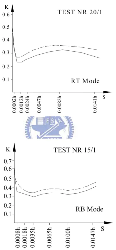
Fig. 2.16 Active earth pressure coefficient under T mode with wall movement (after Bros, 1972) ...76

ix

Fig. 2.17 Active earth pressure coefficient under both RT and RB mode with wall movement (after Bros, 1972)...77 Fig. 2.18 Shaking table, soil box, and actuator (after Sherif et al., 1982) ...78 Fig. 2.19 Shaking table with movable retaining wall (after Sherif et al., 1982) ...79 Fig. 2.20 Ksh, (h/H)s, and tanδ versus wall displacement S (after Sherif et al.,

1982)...80 Fig. 2.21 Experimental KSah values at S /H=0.001 versus soil density (after Sherif

et al., 1982)...81 Fig. 2.22 Change of normalized lateral pressure with wall rotation about top

(loose backfill) (after Fang and Ishibashi, 1986)...82 Fig. 2.23 Distributions of horizontal earth pressure at different wall rotation

(rotation about top ) (after Fang and Ishibashi, 1986) ...83 Fig. 2.24 Distributions of horizontal earth pressure at different wall rotation

(rotation about base ) (after Fang and Ishibashi, 1986) ...84 Fig. 2.25 Horizontal earth pressure coefficient Kh, relative height of resultant

pressure application h/H, and coefficient of wall friction tanδ Versus

wall rotation(rotation about base ) (after Fang and Ishibashi. 1986) ...85 Fig. 2.26 Change of normalized lateral pressure with translation wall

displacement (after Fang and Ishibashi, 1986) ...86 Fig. 2.27 Distributions of horizontal earth pressure at different wall displacement

(after Fang and Ishibashi, 1986) ...87 Fig. 2.28 Coefficient of horizontal active thrust as a function of soil density (after

Fang and Ishibashi, 1986)...88 Fig. 2.29 (S/H)a versus backfill inclination (after Fang et al., 1997) ...89

x

Fig. 2.30 Active earth pressure coefficient Ka,h versus backfill inclination (after

Fang et al., 1997)...90

Fig. 2.31 Hand-calculation for estimating σ_h (after Peck and Mesri, 1987) ...91

Fig. 2.32 National Chiao Tung Univ. non-yielding retaining wall facility ...92

Fig. 2.33 Distribution of vertical earth pressure mearsured in soil mass (after Chen, 2003) ...93

Fig. 2.34 Stress path of a soil element under compaction (after Chen, 2003) ...94

Fig. 2.35 Distribution of horizontal earth pressure after compaction (after Chen, 2003)...95

Fig. 2.36 (a) Bearing capacity failure in soil due to compaction; (b) Modes of bearing capacity failure in sand (Chen, 2003) ...96

Fig. 3.1 Active wall movement modes, (a) Rotation about wall top (RT mode); (b) Rotation about wall base (RB mode); (c) Translation (T mode) (after Huang, 2003) ...97

Fig. 3.2 (a) Rotation about a point above wall top (RTT mode); (b) Rotation about a point below wall base (RBT mode) (after Huang, 2003)...98

Fig. 3.3 Steel interface plate (2100 mm × 1497mm) (after Wang, 2005) ...99

Fig. 3.4 Supporting frame (after Chen, 2005)...100

Fig. 3.5 Different interface inclinations...101

Fig. 3.6 Critical condition for d = 0 mm and α = 45° ...102

Fig. 3.7 NCTU KA model retaining wall ...103

Fig. 3.8 Top view of NCTU KA model retaining wall ...104

Fig. 3.9 Side wall reinforcment ...105

Fig. 3.10 End wall reinforcement ...106

xi

Fig. 3.12 Relationship of the coefficient of earth pressure, K, and the mean wall

displacement, S (after Ichihara and Matsuzawa, 1973) ...108

Fig. 3.13 Typical cross-section of the beam ...109

Fig. 3.14 Dimensions of model retaining wall...110

Fig. 3.15 Model retaining wall ...111

Fig. 3.16 Design of roller supports and unidirectional notches ...112

Fig. 3.17 roller supports and unidirectional notches...113

Fig. 3.18 Gap between model wall and fixed bed...114

Fig. 3.19 Soil pressure transducer (Kyowa PGM-0.2KG) ...115

Fig. 3.20 arrangement of soil pressure transducers...116

Fig. 3.21 Geometry of the wall rotation about the top...117

Fig. 3.22 Geometry of the wall rotation about the base...118

Fig. 3.23 Acrylic cover to protect driving system ...119

Fig. 3.24 Wall-driving system...120

Fig. 3.25 Hinge-and-slider...121

Fig. 3.26 Servo motor of driving system ...122

Fig. 3.27 Speed reducer and worm gear linear actuators of driving system ...123

Fig. 3.28 Control panel of wall driving system ...124

Fig. 3.29 Touch control LCD display ...125

Fig. 3.30 Inductive proximity switch and limit switch ...126

Fig. 3.31 Data acquisition system...127

Fig. 4.1 Grain size distribution of Ottwa sand...128

Fig. 4.2 Shear box of direct shear test device (after Wu, 1992)...129

Fig. 4.3 Relationship between unit weight γ and internal friction angle φ (after Chang, 2000) ...130

xii

Fig 4.4 Pluviation of the Ottawa sand into soil bin ...131

Fig. 4.5 Relationship between relation density and drop height (after Ho, 1999) ...132

Fig. 4.6 Side-view of vibratory soil compactor ...133

Fig. 4.7 Square vibratory soil compactor...134

Fig. 4.8 Backfill compacted with square compactor in 6 lanes ...135

Fig. 4.9 Compaction of backfill with square compactor ...136

Fig. 4.10 Soil-density control cup...137

Fig. 4.11 Soil-density cup ...138

Fig. 4.12 Soil density cups buried at the different elevations ...139

Fig. 4.13 Locations of soil density cups at the elevation ...140

Fig. 4.14 Distribution of soil density compacted with square compactor...141

Fig. 4.15 Relative density vs. Depth relation for vibratory roller compaction (after D’Appolonia et al., 1969) ...142

Fig. 4.16 Lubrication layer on the side wall ...143

Fig. 4.17 Schematic diagram of sliding block test (after Fang et al., 2004) ...144

Fig.4.18 Sliding block test apparatus (after Fang et al., 2004) ...145

Fig. 4.19 Variation of interface friction angle with normal stress (after Fang et al., 2004)...146

Fig. 4.20 Direct shear test arrangement to determine wall friction angle ...147

Fig. 4.21 Relationship between unit weight...148

Fig. 4.22 Relationship between unit weight γ and different friction angles ...149

Fig. 5.1 Variation of wall movements during compaction of backfill...150

Fig. 5.2 Variation of (S/H)a for backfill with different internal friction angle ...151

xiii

Fig. 5.4 Distribution of horizontal earth pressure (Test 0826)...153

Fig. 5.5 Distribution of horizontal earth pressure (Test 0827)...154

Fig. 5.6 Distribution of horizontal earth pressure (Test 0829)...155

Fig. 5.7 Distribution of lateral earth pressure from different tests at S/H = 0.001 ...156

Fig. 5.8 Distribution of lateral earth pressure from different tests at S/H = 0.002 ...157

Fig. 5.9 Distribution of lateral earth pressure from different tests at S/H = 0.003 ...158

Fig. 5.10 Variation of Kh as a function of wall movement...159

Fig. 5.11 Location of total soil thrust as a function of wall movement ...160

Fig. 5.12 Activeearth pressure coefficient K_a,h for soils with different internal frction angles ...161

Fig. 5.13 Surface crack of active failure (S/H=0.016) ...162

Fig. 5.14 Surface crack of active failure (S/H=0.016) ...163

Fig. A1 Schematic diagram of the soil pressure transducer calibration system. ...167

Fig. A2. Soil pressure transducer calibration system...168

Fig. A3. Applied pressure versus voltage output for soil pressure transducer SPT01 and SPT02 ...169

Fig. A4. Applied pressure versus voltage output for soil pressure transducer SPT03 and SPT04 ...170

Fig. A5. Applied pressure versus voltage output for soil pressure transducer SPT05 and SPT06 ...171

Fig. A6. Applied pressure versus voltage output for soil pressure transducer SPT07 and SPT08 ...172

Fig. A7. Applied pressure versus voltage output for soil pressure transducer SPT09 and SPT10 ...173

xiv

List of Symbols

Cu : Uniformity Coefficient

emax : Maximum Void Ratio of Soil

emin : Minimum Void Ratio of Soil

F : Force

Gs : Specific Gravity of Soil

h : Location of Total Thrust H : Effective Wall Height

i : Slop of Ground Surface behind Wall Ko : Coefficient of Earth Pressure At-Rest

Ka : Coefficient of Active Earth Pressure

Kh : Coefficient of Horizontal Earth Pressure

Ka,h : Coefficient of Horizontal Active Earth Pressure

Pa : Total Active Force

RT : Rotation about Wall Top

RTT : Rotation about a Point above Wall Top RB : Rotation about Wall Base

RBT : Rotation about a Point below Wall Base σh : Horizontal Earth Pressure

σN : Normal Stress

S : Wall Displacement T : Translation

z : Depth from Surface

γ _{: Unit Weight of Soil}

φ : Angle of Internal Friction of Soil δ : Angle of Wall Friction

1

Chapter 1

Introduction

Retaining walls are frequently used to hold back the earth and maintain a difference in the elevation of the ground or water surface. In highway constructions, retaining structures are used along cuts or fills where space is inadequate side slopes. Bridge abutments and foundation walls that must support earth fills are also designed as retaining structures. Fig. 1.1 shows the common uses of retaining walls.

The lateral earth pressure induced by active wall movements has been studied with experimental methods by different researchers (Terzaghi, 1934; Macky and Kirk,1967; Bros, 1972; Sherif et al., 1984; Fang and Ishibashi, 1986, and Fang et al., 1997). Terzaghi (1934) noted that backfill compaction significantly affected lateral earth pressures and resulting structure deflections. From an engineering point of view, the active earth pressure distribution behind the wall has a great influence on the adequate design of the retaining structures. It affects not only the bending moment and shear stress distributions within the body, but also the safety of the structure. Therefore, the active earth pressure and the earth pressure induced by compaction become the subject of this study.

2

1.1 Objective of Study

Traditionally, civil engineers build the retaining structures to resist the active force. In most cases, civil engineers calculate the active earth pressure behind a retaining wall using either Coulomb's or Rankine's theory. They assume that earth pressure distribution is linear, and the location of resultant force is located at one third of the wall height above the wall base. Another method to estimate the active and passive earth pressure acting on a retaining structure is the general wedge theory (Terzaghi, 1941). However, this method is a little more complicated, and the estimated active earth pressure is close to the value determined with Coulomb theory (Morgenstern and Eisenstein, 1970).

For granular soils, achieving a relative density of 70~75% is generally recommended (NAVFAC DM-7.2, US Navy 1982). Therefore, the backfill encounterd in the field would be dense soil. Hand tampers and vibratory compaction equipments are commonly used to compact the fill. Terzaghi (1934) reported that compaction efforts would influence the magnitude and distribution of lateral earth pressure. Peck and Mesri (1987) presented a method to evaluate the compaction induced earth pressure.

In Fig. 1.2, the active earth pressure is considered to push the wall. How does the active wall movement affect the compaction-induced earth pressure? Is the design of retaining structures based on the Coulomb’s active earth pressure theory totally appropriate? This becomes the main subject of investigation in this study.

3

1.2 Research Outline

The investigation has been conducted with a newly designed KA model

retaining wall facility in the Foundation Engineering Model Laboratory of National Chiao Tung University. The theories and experimental findings associated with active earth pressure are introduced in Chapter 2. The design of the NCTU KA

model retaining wall facility is discussed in Chapter 3.

Tests results regarding the characteristics of backfill and interface behavior are summarized in Chapter 4. Soil density control experiment were conducted to study soil density distribution in the backfill. Tests results are disscussed in Chapter 4.

In Chapter 5, test results regarding earth pressure due to vibratory compaction and active wall movement were discussed. The backfill with a relative desity of 75% was achieved by compaction method. The variations of lateral earh pressure, total soil thrust, and its point of application as a function of active wall movement are reported. Tests results are compared with the well-known Rankine and Coulomb theories. Based on the experimental results, an estimation of active earth pressure for a compacted cohesionless backfill is suggested.

4

1.3 Organization of Thesis

This thesis is divided into the following parts:

1. Review of theories regarding the active earth pressure and model retaining wall tests. (Chapter 2)

2. A detail description for the design of NCTU KA model retaining wall.

(Chapter 3)

3. Discussion of backfill characteristics and interface characteristics. (Chapter 4)

4. Experimental results regarding the reduction of compaction induced earth pressure with active wall movement. (Chapter 5)

5

Chapter 2

Literature Review

The Coulomb and Rankine earth pressure theories are often applied methods to calculate the lateral force of earth pressure acting on a retaining wall. Experimental studies of active earth pressure have been reported by Terzaghi (1934), Mackey and Kirk (1967), Bros (1972), Sherif et al. (1982), Fang and Ishibashi (1986), and Fang et al.(1997). The major findings of these researches are summarized in this chapter.

2.1 Active Earth Pressure Theories

2.1.1 The Coulomb Theory

Coulomb (1776) proposed a method of analysis that determines the resultant horizontal force on a retaining system for any slope of wall, wall friction, and slope of backfill. The Coulomb theory is based on the assumption that soil shear resistance develops along the wall and failure plane. Detailed assumptions are made as the followings:

1. The backfill is isotropic and homogeneous.

2. The rupture surface is plane, as plane BC in Fig. 2.1(a). The backfill surface is a plane surface as well.

3. The frictional resistance is distributed uniformly along the rupture surface. 4. Failure wedge is a rigid body.

6

5. There is a friction force between soil and wall when the failure wedge moves toward the wall.

6. Failure is a plane strain condition.

To create an active state, the wall is designed moved away from the soil mass. If the wedge ABC in Fig. 2.1(a) moves down relatively to the wall, and the wall friction angle δ will develop at the interface between the soil and wall. Let the weight of wedge ABC be W and the force on BC be F. With the given value θ , and the summation of verticle forces and horizontal forces, the resultant soil thrust P can be calculated as shown in Fig. 2.1(b).

To test different wedge scenarios, the corresponding values of P can be acquired. The upper part of Fig. 2.2 illustrates the curve of P according to different wedge scenarios. And the maximum P is the Coulomb's active force Pa as Eq. (2.1).

a a H K P 2 2 1_γ = (2.1) where

Pa = total active force per unit length of wall Ka = coefficient of active earth pressure

γ _{= unit weight of soil}

H = height of wall and 2 2 2 ) sin( ) sin( ) sin( ) sin( 1 ) sin( sin ) ( sin ⎭ ⎬ ⎫ ⎩ ⎨ ⎧ + − − + + − + = i i K_a β δ β φ δ φ δ β β β φ (2.2)

7

where

φ _{= internal friction angle of soil} δ _{= wall friction angle}

β _{= slope of back of the wall to horizontal}

i = slope of ground surface behind wall

2.1.2 The Rankine Theory

Rankine (1875) considered the soil in a state of plastic equilibrium and used essentially the same assumptions as Coulomb. The Rankine theory assumes that there is no wall friction and failure surfaces are straight planes, and that the resultant force acts parallel to the backfill slope. Detailed assumptions are made as the followings:

1. The backfill is isotropic and homogeneous.

2. Retaining wall is a rigid body. The wall surface is vertical to the ground and the friction force between the wall and the soil is neglected.

3. Elastic equilbrium is not applicable to the stress condition in the failure wedge.

Rankine assumed there is no friction between wall surface and backfill, and the backfill is cohesionless. The earth pressure on plane AB of Fig. 2.3(a) is the same as that on plane AB inside a semi-infinite soil mass in Fig. 2.3(b). For active condition, the active earth pressure σ_a at a given depth z can be expressed as:

a a γzK

σ = (2.3)

8 a a H K P 2 2 1_γ = (2.4)

The direction of resultant force Pa is parallel to the ground surface as Fig.

2.3(b), where ) cos (cos cos ) cos (cos cos cos 2 2 2 2 φ φ − + − − = i i i i i K_a (2.5)

2.1.3 The Terzaghi Theory

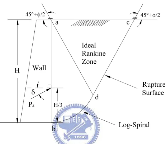
The assumption of plane failure surface made by Coulomb and Rankine, however, does not apply in practice. Terzaghi (1941) suggested that the failure surface in the backfill under an active condition was a log spiral curve, like the curve bd in Fig. 2.4, but the failure surface dc is still assumed plane.

The illustration in Fig. 2.5 shows how Terzaghi and Peck (1967) calculated the active resistance with trial wedge method. The line d1c1 makes an angle of

2

45o +φ _{with the surface of the backfill. The arc bd}

1 of trial wedge abd1c1 is a

logarithmic spiral formulated as the following equation

φ θtan 0 1 re

r = (2.6)

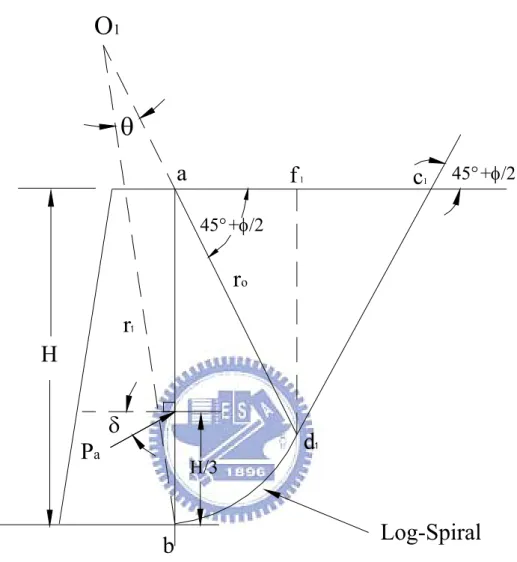
O1 is the center of the log spiral curve in Fig. 2.5, where O1b = r1, O1d1 = r0,

and ∠bO1d1 = θ. For the equilibrium and the stability of the soil mass abd1f1 in

Fig. 2.6, the following forces per unit width of the wall are considered. 1. Soil weight per unit width in abd1f1: W1 = γ × (area of abd1f1)

9

2. The resultant force Pd1 in the zone of Rankine’s active state, acting horizontally on the vertical face d1f1 at a distance of Hd1/3 upward from d1: ) 2 45 ( tan ) ( 2 1 2 2 1 1 φ γ °− = _d d H P (2.7) where Hd1 = d1f1

Pd1 acts horizontally at a distance of Hd1/3 measured vertically upward form d1.

3. The resultant force of the shear and normal forces dF, acting along the surface of sliding bd1. At any point of the curve, according to the property of the logarithmic spiral, a radial line makes an angle φ with the normal. Since the resultant dF makes an angle φ with the normal to the spiral at its point of application, its line of application will coincide with a radial line and will pass through the point O1.

4. The active force per unit width of the wall P1. P1 acts at a distance of H/3 measured vertically form the bottom of the wall. The direction of the force P1 is inclined at an angle δ with the normal drawn to the back face of the wall.

5. Moment equilibrium of W1, Pd1, dF and P1 about the point O1:

[ ]

[ ]

[ ]

1 l P l dF (0) P l

W + _d + = (2.8)

10

[

]

where l_2, l_{3, and} l_{1 are the moment arms for forces W1, Pd1,}

and P1, respectively.

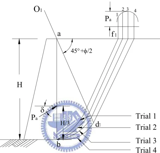
The trial active forces per unit width in various trial wedges are shown in Fig. 2.7. Let P1, P2, P3, …, and Pn be the forces that respectively correspond to the trial

wedges 1, 2, 3, …, and n. The forces are plotted to the same scale as shown in the upper part of the figure. A smooth curve is plotted through the points 1, 2, 3, …, n. The maximum P1 of the smooth curve defines the active force Pa per unit width of

the wall.

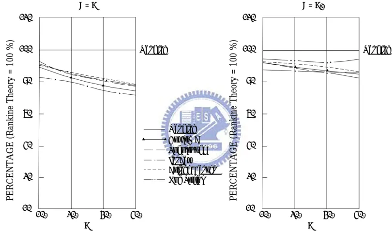
2.1.4 Comparison of Active Earth Pressure Coefficient K

In many theories, the soil mass can be described in a state of limiting equilibrium, and shear strength of soil is expressed with Mohr-Coulomb failure criterion. However, the assumptions differ in the shape of the failure surface. Coulomb (1776) assumed that sliding would occur along a planar sliding surface. Brinch Hansen (1953) assumed the soil wedge slip along a circular surface. Janbu (1957) restricted to a particular shape of slip surface, used the method of slices and satisfied equilibrium in approximate manner. Terzaghi (1941) proposed the logarithmic spiral slip surface.

The coefficient of active earth pressure Ka in different theories were compared

by Morgenstern and Eisenstein (1970). The variation of Ka is the function of

11

equal to φ and φ 2. For the case δ = φ 2, the total range of variation of Ka is

generally less than 15% in Rankine’s solution. In this study, Ka values calculated

with the Coulomb theory and Rankine theory are compared with experiment results.

2.2 Laboratory Model Retaining Wall Tests for Active

State

2.2.1 Model by Terzaghi

Terzaghi (1934) studied the lateral pressure of compacted sand against a large scale model wall at MIT. The face of the wall is 14 ft. in width and 7 ft. in height. The dimension of the soil bin is 14 ft. × 14 ft. × 7 ft. as illustrated in Fig. 2.9. Twenty Goldbeck pressure cells were used to measure the variation of earth pressure, ten built into the wall and ten rested into the floor of the bin. For the wall under translation and rotation about base modes (RB), the earth pressure coefficient K (defined as σ_h γz) was measured at an elevation equal to one-half of

the height of backfill as shown in Fig. 2.10. With a small displacement of the wall, the earth pressure reduced to the fully active state. For a compacted backfill 4.5 ft. in height, an outward displacement of about 1.5 mm (1/1000 of the depth of the backfill) had lead the pressure to an active state. The difference of the K curve for the wall which yields by tilting (Test 1) is not obvious from that of the wall which yields parallel to its original position (Test 2).

Fig. 2.11 shows the relation between the height of the center of pressure (defined as hc/h) and the yield of the wall. According to Coulomb’s theory, the

12

resultant force for level backfill should be located at one-third of the backfill depth above the base (hc/h= 0.33). For rotation about base modes (Tilting wall, RB)

mode, the height of center of pressure is decreased when the wall starts to move. However, after the wall movement equals to 0.00036h, the height of center of pressure gradually rises with the increasing wall movement.

2.2.2 Model by Mackey and Kirk

Mackey and Kirk (1967) experimented on lateral earth pressure by using a steel model wall. This soil tank was made of steel with internal dimension of 36 in. × 16 in. × 15 in. as shown in Fig. 2.12. In their observation, when the wall moved away from the soil, the earth pressure decreased (see Fig. 2.13) and then increased slightly to reach a constant value. Mackey and Kirk concluded that if the backfill is loose, the obtained active earth pressure would be within 14 percent off those theoretical values by the methods listed in Table 2.1.

Mackey and Kirk utilized a powerful beam of light to observe the failure surface in the backfill. It could trace the position of the shadow, formed by changes of the sand surface in different level. It was found that the failure surface due to the translational wall movement was a curve in the backfill (Fig. 2.14), rather than a plane assumed by Coulomb.

2.2.3 Model by Bros

Bros (1972) experimented on various movements of model retaining wall to find the influence by the values and distribution of active and passive earth

13

pressures. The model arrangement is illustrated in Fig. 2.15. The main structure consists of three vertical steel-frames supporting the soil bin, which is 0.7 m in width, 0.85 m in height, and 1.6 m in length. The pressure cells are diaphragm type. The earth pressures were measured with the deforming diaphragm with electric-resistivity strain gauges. In the study, clean, dry, quartz sand from Odra-river was used. The dense state was obtained by vibrating sand of each 12-15 cm layer with electric vibrator.

The outward translation of the wall caused the mobilization of friction between the backfill and side-wall, which tends to decrease the measured lateral pressures. The coefficient of horizontal earth pressure K as a function of wall displacement S is shown in Fig.2.16. It was concluded that the active condition was reached at the wall displacement of 0.0006h (h = height of backfill) under a translational mode. Fig. 2.17 shows that the active conditions are reached at the wall displacement of 0.0035h and 0.0012h~0.0018h, under RB and RT mode respectively.

2.2.4 Model by Sherif, Ishibashi, and Lee

Sherif et al. (1982) compared their experiment results of active static and dynamic earth pressure with Coulomb and Mononobe-Okabe equations. Their experiments were conducted at the University of Washington. The model system consists of four components: (1) shaking table and soil box; (2) loading and control units; (3) retaining wall; and (4) data acquisition system.

14

2.18(a). It was made of steel. The rigid soil box of 2.4 m in length, 1.8 m in width, and 1.2 m in height was built on the shaking table. The movable model retaining wall and its driving system are shown in Fig. 2.19. The model wall consists of the main frame and the center wall. The center wall was 1 m in width, 1 m in height, and 0.127 m in thickness. Six soil pressure transducers were mounted on the center line of the wall surface at different depths to measure the soil pressure distribution against the main body of the center wall (Fig. 2.18b).

Fig. 2.20 illustrates different values of Ksh, h/H and tanδ relative to wall

displacements, where δ is wall friction angle, (h/H) represents the point of application of the soil thrust, and Ksh is the static horizontal coefficient of earth

pressure. The density of the loose Ottawa sand is ρ =1.54 g/cm3_{, and the}

corresponding angle φ is 31.5°. The speed of wall movement stayed constant as 1.5 x10-3 in/sec. The pattern of wall movement was translational. In Fig. 2.20, the Kh value of loose soil gradually decreases until the displacement of the wall

movement is significant. The value of Kh remains stable regardless of the soil

density after the displacement reaches H/1000. Sherif et al. concluded that the experiment Ka,h showed obvious correlation with the Coulomb theory, shown as

Fig. 2.21.

2.2.5 Model by Fang and Ishibashi

Fang and Ishibashi (1986) conducted their experiments with respect to the distribution of the active stresses applying three different wall movement modes: (1) rotation about top, (2) rotation about heel, and (3) translation. Their

15

experiments were also conducted at the University of Washington.

In Fig. 2.22, there is a sharp fall in the pressure behind the lower pressure transducer SPT3, SPT4, SPT5 and SPT6 with wall rotation. And then it stays constant. On the other hand, there is an initial increase in the upper transducer SPT1 and SPT2 with increasing wall rotation. The possible reason may be the arching formed in the upper portion of the backfill soil. Figure 2.23 shows the typical change of lateral stress distribution in different stages of wall rotation. It shows that the arching phenomenon dominates the backfill performance behind the upper portion of the wall when wall rotated about the top.

Figure 2.24 shows the typical horizontal pressure distribution behind a wall rotated about the base. It shows that the lateral pressure of the upper elevation decreases very quickly. However, there is only a very gentle decline in the lateral pressure near the base of the wall with wall rotation. The fully active state is difficult to be reached near the base. In brief, the value of horizontal earth pressure coefficient Kh drops dramatically at the beginning and then keeps constant.

Accordingly the total thrust in Fig. 2.25 is not be able to return to the position of H/3 above the bottom of the wall, which means the existence of the remaining part of the extra stress near the base of the wall.

Figure 2.26 shows the lateral earth pressure measured at various depths. The lateral pressure falls rapidly due to the translational wall displacement. Most of the measurements reach the minimum value at approximately 10 10_× −3

in. (0.25 mm) wall displacement and then stay stable thereafter.

16

Figure 2.27 shows the horizontal earth pressure distributions at different translational wall movements. The measured active stress is slightly higher than Coulomb's solution at the upper one-third of wall height, approximately in agreement with Coulomb's prediction in the middle one-third, and lower than Coulomb' at the lower one-third of wall surface. However, the magnitude of the active total thrust Pa at S = 20 10_× −3

in. (0.5 mm) is almost the same as the value calculated apply to the Coulomb theory.

Figure 2.28 shows the Ka is the function of soil density and internal friction

angle. The value of Ka decreases while the angle of φ increases. There might be a

underestimation of the coefficient Ka in Coulomb’s solution for rotational wall

movement.

2.2.6 Model Study by Fang et al.

Fang et al. (1997) presented experimental data of earth pressure acting against a vertical rigid wall, which moved away from or toward a mass of dry sand with an inclined surface. The instrumented NCTU retaining-wall facility was used to investigate the variation of earth pressure induced by the translational wall movement.

Based on their experimental data, it has been found that the earth-pressure distribution is essentially linear at each stage of wall movement. As shown in Fig. 2.29, the wall movement required for the loose backfill to reach an active stage increase with an increasing backfill inclination. Fig. 2.30 shows the experimental active earth-pressure coefficients for various backfill sloping angles are in good

17

agreement with the values calculated by Coulomb’s theory. It may be observed in the figure that it is not appropriate to adopt the Rankine theory to determine active earth pressure against a rigid wall with sloping backfill.

2.3 Effects of Soil Compaction in Earth Pressure

Compaction a soil can produce a stiff, settlement-free and less permeable mass. It is usually accomplished by mechanical means that cause the density of soil to increase. At the same time the air voids are reduced and the coordination number of the grains is increased. It has been realized that the compaction of the backfill material has an important effect on the earth pressure on the wall.

Several theories and analytical methods have been proposed to analyze the residual lateral earth pressures induced by soil compaction. Most of these theories introduce the idea that compaction represents a form of overconsolidation, where stresses resulting from a temporary or transient loading condition are retained following removal of this load.

2.3.1 Study of Peck and Mesri

Based on the elastic analysis, Peck and Mesri (1987) presented a calculation method to evaluate the compaction-induced earth pressure. The lateral pressure profile can be determined by four conditions on σh, as illustrated in Fig. 2.31 and

summarized in the following.

18

z

h φ γ

σ =(1−sin ) (2.10)

2. Lateral pressure limited by passive failure condition,

z

h φ γ

σ ₌tan2(45₊ /2) _(2.11)

3. Lateral pressure resulting from backfill overburden plus the residual horizontal stresses, h h φ γz σ σ _{= − + (5} φ _−1)∆ 4 1 ) sin 1 ( 1.2sin _(2.12)

where ∆σh is the lateral earth pressure increase resulted from the surface

compaction loading of the last backfill lift and can be determined based on the elastic solution.

4. Lateral pressure profile defined by a line which envelops the residual lateral pressures resulting from the compaction of individual backfill lifts. This line can be computed by Eq. 2.13

γ φ σ _{(5 5} φ₎ 4 sin 1− ₋ 1.2sin = ∆ ∆ z h _(2.13)

Fig. 2.31 indicates that near the surface of backfill, from point a to b, the lateral pressure on the wall is subject to the passive failure condition. From b to c, the overburden and compaction-induced lateral pressure profile is determined by Eq. 2.12. From c the lateral pressure increases with depth according to Eq. 2.13 until point d is reached. Below d, the overburden pressure exceeds the peak stress in effective in compaction. In the lower part of the backfill, the lateral pressure is directly related to the effective overburden pressure.

19

2.3.2 Study of Chen

Chen (2003) reported some experiments in non-yielding retaining wall at National Chiao Tung University (Fig. 2.32) to investigate influence of earth pressure due to vibratory compaction. Air-dry Ottawa sand was used as backfill material. Vertical and horizontal stresses in the soil mass were measured in loose and compacted sand. Based on his test results, Chen (2003) proposed four points of view: (1) the compaction process does not result in any residual stress in the vertical direction. The effects of vibratory compaction on the vertical overburden pressure are insignificant, as indicated in Fig. 2.33 and Fig. 2.34; (2) after compaction, the lateral stress measured near the top of backfill is almost identical to the passive earth pressure estimated with Rankine theory (Fig. 2.35). The compaction-influenced zone rises with rising compaction surface. Below the compaction-influenced zone, the horizontal stresses converge to the earth pressure at-rest, as indicated in Fig. 2.35(e); (3) when total (static + dynamic) loading due to the vibratory compacting equipment exceeds the bearing capacity of foundation soils, the mechanism of vibratory compaction on soil can be described with the bearing capacity failure of foundation soils (Fig. 2.36); (4) the vibratory compaction on top of the backfill transmits elastic waves through soil elements continuously. For soils below the compaction-influenced zone, soil particles are vibrated. The passive state of stress among particles is disturbed. The horizontal stresses among soil particles readjust under the application of a uniform

20

overburden pressure and constrained lateral deformation, and eventually converge to the at-rest state of stress.

21

Chapter 3

Design of NCTU K

A

Model Retaining Wall

Facility

The design of NCTU KA model retaining wall facility are discussed in this

chapter. The model wall in this study is assumed a rigid body, such as a gravity retaining wall. At the beginning of design, two important testing parameters have been considered: (1) the wall height, and (2) the maximum wall displacement.

The KA model wall facility is designed to investigate active earth pressure. At

the same depth Z, the active earth pressure (σ_a =K_aγZ ) would be smaller than the

earth pressure at rest (σ_o = K_oγZ ). Consequently, it is necessary to increase the

wall height (increase the overburden pressure) in order to obtain more obvious experimental σ_a data. According to the space available in the NCTU foundation model lab, the effective wall height H (actually the height of backfill) was evaluated and selected to be 1.0 m.

It is important for the designer to consider how much wall displacement is required to achieve an active state in the backfill. Table 3.1 shows the range of wall displacement reported by previous researchers for different wall movement modes to achieve an active state of stress. Based on their studies, the wall displacements from 0.0005H to 0.0040H could lead to active states. The NCTU KA Model

Retaining Wall is designed to observe the active failure surface in the backfill. Fang (1983) reported that the surface failure cracks appeared when the wall

22

displacement reached H/150. With a factor of safety of 3.0, H/50 (20 mm) was selected as the largest active displacement for the model wall.

3.1 Design Motivation

In order to study the variation of earth pressure more extensively, the KA

model wall facility was proposed. This newly designed and constructed retaining wall to investigate active earth pressure has the following features:

3.1.1 Large-scale model wall

The previous NCTU model wall was designed for both active and passive earth pressure experiments. Subjected to tremendous passive earth pressure acting on the model wall, the height of the wall was limited to 0.5 m. However in the new design, the wall is designed mainly for active earth pressure experiments. The earth pressure would decrease from at-rest to active state of stress. The increased height of 1.0 m to enhance the investigation range of lateral earth pressure distribution. With the new facility, the effects of compaction on earth pressure can now be observed in both shallow and deeper location.

3.1.2 Wall driven by servo motors

The servo motor can accurately control both of the velocity and position of the model wall. In the previous retaining wall experiments, the start and stop of model wall were controlled manually. For the new KA model wall experiments, the

23

3.1.3 Large wall displacement

The cracks on the soil surface can be observed only at a large active wall movement. With the large wall displacement (S = 20 mm) design for the new model wall, the earth pressure due to the backfill in a critical state can also be investigated.

3.2 Types of Experiments

The KA model wall facility is designed for various types of earth pressure

experiment. Possible research subjects with the new model wall are summerized as the follows:

1. Relative density of backfill

The intensity and distribution of active earth pressure acting on the wall would be affected by the relative density of soil. Experimental methods such as air-pluviation and soil compaction can be used to create different backfill densities. 2. Wall movement mode

With the new model wall, five types of active wall movement modes are possible: (1) rotation about the wall top (RT mode, Fig. 3.1(a)); (2) rotation about the wall base (RB mode, Fig. 3.1(b)); (3) translation mode (T mode, Fig 3.1(c)); (4) rotation about a point above wall top (RTT mode, Fig. 3.2(a)),and (5) rotation about a point below wall base (RBT mode, Fig. 3.2(b)).

24

(4) and (5) modes. 3. Adjacent stiff rock face

Wang (2005) and Chen (2005) designed and consa supporting system of the steel interface plate (Fig. 3.3) and the supporting frames (Fig. 3.4) to simulate the effect of adjacent rock face behind the retaining wall, as shown in Fig. 3.5. Various scenarios of interface installations were simulated. This interface plate was integrated in the NCTU KA model retaining wall. Hence, the effect of the rock face

can also be simulated. And the distribution of earth pressure can be observed in active state.

4. Step movements of wall

When a retaining wall is built in the field, it is necessary to fill up and then compact the backfill behind the wall in layers. The wall displacement would occur progressively during the filling and compaction of backfill. Therefore, in order to simulate the field condition, it would be interesting to investigate the variation of earth pressure due to the step movements of retaining wall.

3.3 NCTU K

Model Retaining Wall Facility

The entire NCTU KA model retaining wall facility consists of four components,

namely: (1) soil bin; (2) model wall; (3) driving system; and (4) data acquisition system. The design of these components are introduced in the following sections.

25

3.3.1 Soil Bin

1. Length of Soil Bin

Fig. 3.6 shows, for H=1.0m, the length of active failure wedge approximates to 577 mm based on the Rankine theory. Loose backfill condition is considered with an inertial friction angle of 30 degrees. The soil bin is designed to simulate the intrusion adjacent rock face behind the wall as shown in Fig. 3.6. In Fig. 3.6, with the steel interface plate inclined at α = 45°, the length of soil bin at the top of the model wall should be at least 1.2 m. The design length of the soil bin is 1.5m, to tolerate possible uncertainties.

2. Width of Soil Bin

The selection of the width of the soil bin used to hold the backfill is governed by the friction effect along the side walls. Terzaghi (1932) experimented on small-scale tests in several model retaining walls and suggested the adequate length of the wall twice as long as the depth of the fill.

The width (W) of the soil bin for this study is set to be 1.5 m, which is 1.5 times of the the backfill height. To efficiently reduce the side-wall frictional effect, a lubrication layer fabricated with plastic sheets is placed between the backfill and the side wall. The measured friction angle at the soil-sidewall interface with this method is about δ =7.5°. With the design considerations mentioned, the side wall friction effect on K will be effectively reduced. _a

3. Structure of Soil Bin

26

1100 mm as shown in Fig. 3.7 and 3.8. The major concern to choose the material is rigidity. Both sides of the soil bin are made with 30 mm-thick transparent acrylic plates. Therefore, the behavior of the backfill during shear can be observed. Fig. 3.9 shows outside the acrylic plates, U-shaped steel beams with steel columns of 20 mm in thickness were welded. In this way the lateral displacement of the acrylic side wall will be constrained during the loading process. The side walls are confined laterally to ensure the plane strain condition in the backfill. For observing the active failure wedge in the soil mass, a spacious clearence (600mm-wide) is reserved without steel reinforcements. The reinforcement of end wall with steel beams and columns is illustrated in Fig. 3.10.

The bottom of the soil bin is covered with a layer of SAFETY WALK (3M), which is a anti-slip frictional material. It generates adequate friction between the soil and the base of the bin.The end wall parallel to the model retaining wall is made of a 20 mm thick steel plate. All corners, edges and screw-holes of the soil bin were sealed to avoid leakage.To create a plane strain condition for the model test, the following rules should be followed:

1. Rigidity: The soil bin is nearly rigid that lateral deformation of side wall becomes negligible.

2. Frictionlessness: The friction between the backfill and the side walls should be minimized. The lubrication layer is made of one thick and two thin plastic sheets between the side walls and the soil.

27

3. Uniformity: The properties of backfill should be uniform along the width of the retaining wall. The method to control the uniformity of backfill will be discussed in Chapter 4.

3.3.2 Model Wall

1. Positions of Driving Rods

The positions of the upper and lower wall driving rods are determined based on the distribution of lateral earth pressure, which is assumed linear with depth as shown in Fig. 3.11. The mechanics of materials theories is used to analyze the deflection of wall face. The wall is considered as a beam and a 2-dimensional analysis is made. The discontinuity functions are used to determine beam deflections.The reactions RB and RC in Fig. 3.11 are formulated as

⎟ ⎠ ⎞ ⎜ ⎝ ⎛ _{+ −} = a b H b qH R_B 3 2 2 _, ⎟⎠ ⎞ ⎜ ⎝ ⎛ ₋ = H a b qH R_C 3 2 2 _(3.1) where = B

R _{reaction at upper driving rod}

=

C

R _{reaction at lower driving rod}

=

H _{height of backfill}

=

q _{intensity of lateral pressure at depth H}

=

a _{distance from soil surface to upper driving rods}

=

b _{distance from soil surface to lower driving rods}

Gere and Timoshenko (1984) developed the load intensity q

( )

28

( )

(

)(

)

(

)(

)

(

)(

)

−R_Bu Z a Z a and −R_Cu

(

)(

)

functions, and Z denotes the depth from the soil surface. Substituting R_B and R _C

of Eq. (3.1) in Eq. (3.2), and applying the differential relationship of the external load and beam deflection, the following equation is obtained:

( )

(

)(

)

(

)(

)

Integrating equation (3.3), with the boundary conditions for beam deflection, for translation case.

( )

y , y

(

)

Thus, the final expressions for y

( )

(

)(

)

29

(

)(

)

(

)

(

)

To reduce the maximum wall deflection and generate a relatively uniform distribution of wall deformation, the vertical positions of the wall driving rods are subjected to δ_A =δ_D =δ_E. where = A δ _{deflection at point A} = D δ _{deflection at point D} = E

δ _{max. deflection between point B and point C (deflection at} point E)

The result of Eq. (3.4) with the constrant mentioned is obtained: =

a 360 mm, b= 472.64 mm, Z₁ = 590 mm, where Z₁ = distance from

soil surface to point E. Based on the result above, the upper driving rods are positioned at 360 mm below soil surface, which is 430 mm below the top of the wall. The lower driving rods are positioned at 472 mm below the upper rods.

30

The model wall is designed for active earth pressure tests only. The model wall is designed to resist earth pressure at rest following Jaky’s formula. The lateral earth pressure is computed for dry Ottawa sand which has the unit weight

γ =15.14 kN/m3, with an internal friction angle of φ=30°.

The loading condition of the beam is shown in Fig. 3.11. The intensity of Jaky earth pressure at the base of the wall is calculated as the following:

(

)

(

)

(

)

( )(

)

The maximum deflection of the model wall is calculated from Eq. (3.4):

(

)(

)

(

)(

)

(

)

(

)

31

=

q _{intensity of earth pressure at wall base =11.35kN /m}

=

H _{wall height} =0.5m m

a=0.36 _, b=0.472m_{, and} Z1 =0.59m

the maximum deflection in Eq. (3.4) can be transformed to Eq. (3.5).

q

EIδ_max =9.16×10−5 (3.5)

Ichihara and Matsuzawa (1973) plotted the coefficient of earth pressure K relative to wall displacement S for a 550 mm high wall backfilled with dry uniform sand (Fig.3.12). The wall movement from zero to 0.001 mm in their study (S/H = 0.0000018) corresponds to the value from 0.88 to 0.8772 of K. The ∆ K holds 0.41% of the range between 0.88 and 0.8772. This deformation amount (S/H = 0.0000018) is satisfying since the wall is not a perfectly rigid body. Consequently for the 1000 mm-high NCTU model wall, it can be considered as a rigid wall if the maximum wall deflection is less than 0.0018 mm.

From equation (3.5): q EIδ_max =9.16×10−5

(

)

(

)

(

) (

)

The typical cross section of the loaded beam is shown in Fig. 3.13. For the moment of inertia of the section under consideration:

(

)

32

The NCTU wall thickness should be calculated at least 29 mm to minimize the effect of wall deflection. The final wall thickness of 50 mm is adopted. The thickness of the central part of the model wall is 45 mm for installation of the soil pressure transducers.

3. Structure of Model Wall

Fig. 3.14 and 3.15 shows the dimensions of the model wall. The steel model wall is 1,500 mm wide, 1,070 mm high, and 50 mm thick. The model wall is vertically supported by two rollers. Two driving systems seperately control the upper and the lower driving rods to simulate various kinds of wall movement in the field.

Fig.3.16 and Fig. 3.17 shows two 45-degree notches has been grooved at the bottom of the model wall. Other two notches are grooved on the top of the fixed bed, which is below the wall. The top grooves are located exactly above the bottom ones. Two 30 mm-diameter steel balls allow the model wall to move parallel to the longitude of the soil bin. The gap clearance between the model wall and the fixed bed shown in Fig. 3.18 is influenced by the thickness of the wall and the desired wall rotation angle. A smaller gap can reduce leakage of the backfill during wall movement. The gap width is designed to be 1 mm, corresponding to the wall thickness of 50 mm and the wall rotation of ± 2 . °

The soil pressure transducers are installed on the model wall to observe the distribution of lateral earth pressure. The arrangement of the transducers should be close enough to closely monitor the distribution of pressure changes with depth.

33

Ten soil pressure transducers (Kyowa PGM-02KG) shown in Fig. 3.19 were arranged along the center line of the model wall as shown in Fig. 3.20. In addition, other three transducers were placed between the center line and the side wall to investigate the side wall effects. The soil pressure transducers were built very stiff to eliminate the effects of soil arching. They were flush-mounted to the surface of the model wall.

The NCTU KA model retaining wall can simulate different types of wall

movements. The geometry of the model wall rotation about the top (RT mode) in active state is shown in Fig. 3.21. The lateral movement ratio of the lower driving rods over the upper rods is (360+472)/360 = 2.31. If the maximum horizontal wall movement at the base of the wall is 0.005H (5mm) with the backfill height (H=1000 mm). In this situation, the lower driving rods should move 4.17mm, and the movement is 1.80 mm at the upper rods.

The geometry of the model wall rotation about the base (RB mode) in active state is shown in Fig. 3.22. The lateral movement ratio of the upper driving rods over the lower rods is (472+168)/168=3.81, regardless of the level of soil surface. With the maximum wall movement at the top of backfill 0.005H (5mm), the upper driving rods moves 3.2 mm and the lower rods moves 0.84 mm.

In the experiments, Ottawa sand would be deposited by air-pluviation into the soil bin. An acrylic cover shown in Fig. 3.23 was designed and constructed allocated to protect the servo motor and driving system from dust. An opening was made at the back side of the acrylic cover, so that operators can enter the space to

34

replace soil pressure transducers and set up displacement dial gauges behind the model wall.

3.3.3 Driving System

The driving system is used to push and pull the model retaining wall. It consists of four componets: (1) driving rods; (2) servo motor; (3) control panel; and (4) inductive proximity switch. Fig. 3.24 illustrates the operation of wall driving system, and the details are described in the following sections.

1. Driving Rods

Four driving rods are attached on the model wall to push and pull the model wall. Fig. 3.25 shows the hinge-and-slider connection connecting between the driving rod and the model wall. The connection could keep the driving rod at the same elevation when the model wall rotates.

2. Servo Motor

The servo motor uses feedback signals to control the speed of driving rods accurately. Two servo motors (Sinano Electric 8CB75-2DE7FAS) shown in Fig.3.26 have been installed to propel the upper and lower driving rods independently. The maximum rotation speed of motor is 3000 rpm. In Fig.3.27, two speed reducers (gear ratio 60:1) are installed in front of the motors to control the speed of shaft. The horizontal shaft propel the two worm gear linear actuators (worm gear ratio 16:1). After conversions, it needs 960 revolutions of motor to pull each pitch distance of 8mm. The rotation speed of motor is subject to the capacity of 1PG (AX2n-1PG), which can generate 100,000 pulses per seconds. The motor

35

needs to receive 8000 pulses for each revolution (8000 ppr). Thus the maximum wall speed can be programmed to 0.001 mm/s to 0.1 mm/s through the Programmable Logic Controller (PLC) in the control panel. The speed of driving rod can be easily operated from the touch-control LCD display.

3. Control Panel

The control panel has attached a touch-control LCD display (Fig. 3.28) to input the controlled paramters. There are three operation modes on the control panel to control wall movements. The first mode is to input the speed and running time for upper and lower rods respectively. The second one is to input the positon coodinates of upper and lower driving rods. And the third is to input an additional displacement from present position coodinates. Threrfore, various experimental demands for wall movements can be achieved. In Fig. 3.29, the wall speed and running time can be set on the LCD screen of the control panel.

4. Inductive Proximity Switch

In Fig. 3.30, the inductive proximity switch (IFRM 08N1701/L) and the limit switches are set on the driving rod. The inductive proximity switch detects the position of an object and transforms a electronic signal. The initial position of the metal ring is right below the sensor. After the motor begins to operate, the metal ring starts to move with the same speed as the wall. When the wall returns to the initial position, the inductive switches can sense the matal ring and send a “stop” signal to the servo drive. This mechanism ensures that the model wall will return to its original position after each test.

36

The purpose of limit switches is to prevent unusual operation of motors. If the servo motors do not follow the commands from contorl panel, it will stop the operation of servo motors when metal rings pass through the limit switches.

3.3.4 Data Acquisition System

Due to the considerable amount of data collected by the soil pressure transducers and displacement transducers, a data acquisition system shown in Fig. 3.31 was used for this study. It is composed of the following four parts: (1) dynamic strain amplifiers (Kyowa: DPM601A and DPM711B); (2) NI adaptor card; (3) AD/DA card; and (4) personal computer. The analog obtained signals from the sensors are filtered and amplified by dynamic strain amplifiers. Analog experimental data are converted to digital data by the A/D – D/A card. The LabVIEW program is used to acquire test data. Experimental data are stored and analyzed with a Pentium 4 personal computer.

37

Chapter 4

Backfill and Interface Characteristics

The properties of the backfill (Ottawa sand) the friction between the backfill and the acrylic sidewalls, and the friction between the backfill and the steel model wall are discussed in this chapter. The following sections include: (1) backfill properties; (2) the method to prepare the backfill; (3) the method to control soil density; (4) sidewall friction; and (5) model wall friction.

4.1 Backfill Properties

4.1.1 Characteristics of Backfill

Air-dry Ottawa silica sand (ASTM C-778) is used in the experiments. Table 4.1 lists out the physical properties of Ottawa sand. Grain-size distribution of the backfill is shown in Fig. 4.1. The major reasons to select Ottawa sand as the backfill material are listed below.

1. the round particle shape can avoid problems of angularity,

2. the uniform distribution of grain size (coefficient of uniformity Cu = 1.78) can avoid problems of soil gradation,

3. the high particle rigidity can reduce disintegration of soil particles under loading

4. the high permeability can drain very fast and avoid water pressure against the wall.