pansion of the three-step search algorithm (TSS). It can be seen from the simulation results that the performance of LGSA is very similar to that of FSA, and the computational complexity is much lower than that of FSA and other previously proposed genetic motion estimation algorithms.
Index Terms—Block matching, genetic algorithm, video coding.
I. INTRODUCTION
T
HE block-matching algorithms (BMA’s) have been shown to be very efficient for the reduction of video bit rates [1]. It is therefore widely used in various kinds of video applications. In most of the video coding standards (such as H.261, MPEG-1, and MPEG-2), the block-based motion estimation technique is a key component. Because of its importance, many works have been devoted to the development of fast search algorithms. The full search algorithm (FSA) can find the optimal solution (i.e., the best motion vector) by exhaustively searching all possible blocks, but the required tremendous computations make it difficult to apply for real-time video compression, particularly for software-based implementation. To meet the need of decreasing the computational complexity of the block-matching process, different kinds of fast searching algorithms have been proposed [1]–[5]. Most of these fast algorithms have the restriction or the assumption that there should be only one minimum in the search space. However, in normal cases, there always exist multitudinous local minima in the search space. Frequently, these fast search algorithms will miss the optimal solution, but stick at a suboptimal one. Hence, the performance of these fast search algorithms is always much poorer than that of FSA.In order to amend the performance degradation caused by the assumption of single minimum, Jong [5] proposed a method called the multicandidate three-step search algorithm (MTSS). In this algorithm, a fixed number of least distortion search points (LDP’s), instead of only one, are kept in each iteration step of the TSS. It is shown by simulation results
Manuscript received September 15, 1995; revised October 1, 1996, Decem-ber 19, 1997, and March 23, 1998. This paper was recommended by Associate Editor B. Zeng.
C.-H. Lin is with the Communication and Multimedia Laboratory, Depart-ment of Computer Science and Information Engineering, National Taiwan University, Taipei 106, Taiwan, R.O.C.
J.-L. Wu is with the Communication and Multimedia Laboratory, Depart-ment of Computer Science and Information Engineering, National Taiwan University, Taipei 106, Taiwan, R.O.C., and the Department of Information Engineering, National Chi-Nan University, Puli 545, Taiwan, R.O.C.
Publisher Item Identifier S 1051-8215(98)05761-9.
the number of LDP’s increases, the computational cost also increases, while the performance improves, and vice versa.
On the other hand, all LDP’s are treated equally in MTSS. In other words, all LDP’s derive an identical number of search points, i.e., eight nearest search points. It is possible that an LDP is far from the solution, and has a large matching error. The derived search points from this LDP are therefore also far from the solution. The computations spent on these search points are superfluous.
In previous works [6], [7], genetic algorithms (GA’s) have been used to solve the local minima sticking problem. It is shown from these papers that the performance of GA-based search algorithms is similar to that of FSA. However, the computational complexity of these algorithms is too high to be applied in a video coding system.
In this paper, a lightweight genetic search algorithm is proposed. It is shown by simulation results that the compu-tational complexity is largely reduced while the performance is still maintained, which makes it possible to be used in real systems. This algorithm also has more flexibility than MTSS. The number of LDP’s is dynamically changed in different steps, and different LDP’s can derive different numbers of search points.
II. LIGHTWEIGHTGENETICSEARCHALGORITHM
Let be a solution space, and let all search points in have their associated fitness values. The most straightforward way to find the search point with the maximum fitness value is to search among all search points, and to compare their fitness values. However, the computational complexity will be very high. In order to reduce the computational complexity, an efficient search algorithm is needed.
When GA’s are applied to search for the global maximum in , a population is maintained which consists of search points, where is the population size. Each search point in is represented as a chromosome which is composed of a list of genes. The population will evolve into another population by performing some genetic operations. Chromosomes with higher fitness values will have higher probabilities to be kept in the population of the next generation, and to propagate their offsprings. On the other hand, weak chromosomes, whose fitness values are small, will be replaced by another stronger chromosomes. Therefore, the quality of the chromosomes in the population will improve. When the iteration process converges, the global maximum is expected to be contained in the mature population.
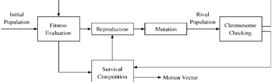
Fig. 1. Structural diagram of the genetic block-matching algorithm.
In video coding applications, the solution space is a set of motion vectors. The th chromosome in the population is defined as
(1) where represents one possible motion vector, and is the codeword size of each motion offset whose value depends on the search range. If the search range is from to pixels, the value of will be , where is the ceiling function. The values of the genes are derived from
, that is (2) (3) and (4) (5)
where mod is the module operation and is the floor function.
Fig. 1 depicts the block diagram of the genetic evolution in LGSA. An initial population is formed before the evolution. Initial chromosomes are selected from fixed locations near the central point of the search space. The candidate motion vector
of the th initial chromosome is
(6) (7) where
(8)
Fig. 2. Initial chromosomes distribute equally on the search space.
(9) (10)
and
(11) For example, when , initial chromosomes are shown in Fig. 2.
Each chromosome has an associated fitness value which is defined as
(12) where is the matching error of the th chromosome, is the retainer number, is the th minimum matching error
among all the values, , and and
are the unit step function and delta function, respectively. Retainer number determines how many chromosomes at most could be selected as the seeds in the reproduction stage for producing a rival population. From (12), it follows that the chromosomes with smaller matching errors will have larger fitness values. Chromosomes with larger fitness values in the current population have higher probabilities to be selected as seeds of the rival population. This probabilistic scheme of selecting seeds of the new generation is known as probabilistic reproduction. Because is either zero or one, no multiplication for computing fitness values is required.
where is the fitness value of the th chromosome in the population, and “ ” and “ ” denote closing and opening boundaries, respectively. When the incidence range of each chromosome has been determined, real numbers are
randomly generated, where and
. The value of will belong to some , that is, . The th chromosome is then selected as a seed. It is possible that one chromosome can be selected twice or more. Because real random numbers are generated, seeds could be selected and placed in the mating pool.
While comparing with the traditional implementation [9], the advantage of this method is that the seeds can be directly indexed, so the control overheads are small. On the other hand, the disadvantage is that divisions are required to calculate the incidence ranges. The computational complexity might be a little higher than that of the traditional methods.
After the reproduction stage, each seed in the mating pool will be processed and transferred into a candidate chromosome of the new generation. Assume that the current seed to be
processed is , where and
. In the th generation, two genes
and are varied, where . There are eight
mutation operators , which can be
applied in our implementation, that is
(14) (15) where is a random integer number whose value is between zero and seven. Because chromosomes are randomly selected and put in the mating pool, it is not necessary to generate a random number for determining the value of . We simply set to be . The mutation operators, which are defined to reach the neighboring eight search points as in TSS, are defined as
(16)
(17) (18) When mutation operators are performed on the most sig-nificant genes of the chromosomes (e.g., , etc.), chromosomes which are far from the original ones in the
values will be picked up as the members of the population in the next generation, and go through the next iteration of the genetic evolution. Because the population size is usually not large in LGSA, we simply sort the chromosomes and select the best ones. This stage is added to the proposed algorithm to prevent the chromosomes from being destroyed by the new ones with poorer fitness values because the new chromosomes generated from the original ones are not guaranteed to have larger fitness values in GA’s.
The chromosome with the maximum fitness value is selected from the current population as the possible solution. The possible solution might be replaced by the others from one generation to the other generations. The iteration will be terminated if the matching error of the possible solution is less than a predefined threshold, or the iteration number is equal to the maximum iteration number . When the search range is from 16 to 15 pixels, the iteration number will less than five. In LGSA, the maximum generation number is adjusted according to the search range. When a larger block size or higher frame rate is used, the generation number will be large due to the existence of more local minima. We do not adjust the maximum generation number according to the block size or frame rate so as not to involve too many computations. The increment of computations will narrow the complexity difference between LGSA and FSA.
LGSA can be summarized as follows.
• Population: The th-generation population
, for has chromosomes
. The initial population is . • Reproduction:
— Compute the fitness value and the range value for each chromosome .
— Choose seeds randomly from based on the range values for mutation.
• Mutation: Generate new mutated chromosomes from the seeds through mutation operators: and . • Survival competition: Sort and newly mutated
chromosomes (total ) in terms of fitness values in a descending order. Pick the first chromosomes as the new generation . Repeat the process until a termination condition is reached.
III. COMPARISONS OFLGSAWITH OTHER BMA’S
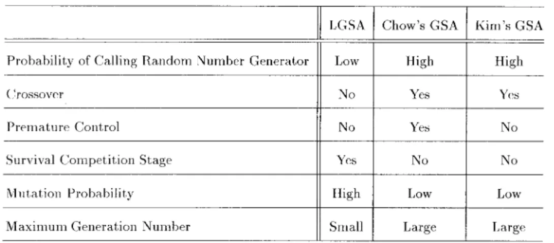
The main differences between LGSA and the other previ-ously proposed genetic search algorithms are listed in Table I. The computational cost to generate a random number is not low. In other applications that apply GA’s, the search space
TABLE I
COMPARISONS OFDIFFERENT GENETICSEARCHALGORITHMS
is usually large, and a time constraint is not so important; hence, the computational cost required to generate random numbers is relatively inexpensive. However, when GA’s are applied to perform block matching, the cost of generating a random number is relatively high because the search space is rather small and a time constraint is very important. In the other two genetic search algorithms, random numbers must be generated in the reproduction, crossover, and mutation stages. Nevertheless, the random number generator is only called in the reproduction stage of LGSA. Therefore, the computational cost is largely reduced.
In Chow’s and Kim’s GSA’s, crossover is applied in the algorithms. The purpose of performing crossover is to ran-domly exploit new search points. Because the search space is not large in BMA’s, there is not a large number of local minima in the search space. The efficiency of crossover is not prominent. Therefore, the crossover stage is not included in LGSA.
In Chow’s GSA, a dynamic population control scheme is involved to avoid premature convergence. There is no similar scheme in LGSA. The maximum iteration number in LGSA is not large, for example, it is equal to four if the maximum motion offset is 16 pixels, so it is improper to apply a similar scheme in LGSA. That control scheme might make the overall fitness of the population decrease. In LGSA, another scheme called survival competition is applied. It ensures that the quality of each chromosome in the current population is better than the old ones.
There are two kinds of mutation operators used in traditional GA-based implementation: 1) changing a gene’s value from zero to one, or 2) from one to zero. Moreover, the mutation probability is usually very low in order not to impair the over-all quality of a population. In LGSA, the mutation probability is very high, and there are many mutation operators, so the evolution of chromosomes is relatively violent. However, the bad effect of a high mutation rate can be avoided because of the survival competition. On the other hand, more search points can be reached due to the high mutation rate, although there is no crossover stage in LGSA.
TABLE II
COMPARISONS OF THEAVERAGEPERFORMANCE INNORMALFRAME
RATE: (a) PERFORMANCE, (b) PERFORMANCEDIFFERENCE FROM
FSA, (c) VARIANCE OFPERFORMANCEDIFFERENCE FROMFSA
(a)
(b)
(c)
Because the evolution of chromosomes is slow in Chow’s and Kim’s algorithms, the maximum and the average gen-eration numbers are large. Moreover, their average block-matching numbers are also large. Hence, both the control overheads and the cost of performing block matching are tremendous. In LGSA, the evolution is relatively violent, and
(a) (b)
(c) (d)
(e)
Fig. 3. Original and predicted images selected from the 36th image of the “Table Tennis” sequence by using different search algorithms in low frame rate: (a) the original image, (b) FSA, (c) TSS, (d) MTSS, (e) LGSA.
the quality of chromosomes is well controlled by the survival competition, so the maximum generation number is small. Therefore, the control overheads of chromosome evolution are reduced. Moreover, the block-matching number of LGSA is relatively small because most of the irrelevant chromosomes are excluded.
In MTSS, a fixed number of search points is retained in each iteration for further probing. The neighboring points of other search points, with least distortion, will never have the chance to be probed. Moreover, all of the retained points, no matter whether the corresponding distortion is large or small, will
derive an identical number of offsprings in the next iteration. In LGSA, a more flexible offspring derivation scheme was applied. The search points with less distortion will have higher probabilities to be retained in the iteration, whereas the ones with larger distortion have fewer probabilities to derive their offsprings. That is, the neighboring points of these larger distortion points still have a chance to be probed. This scheme for determining the retained points makes LGSA more efficient in resolving the local minimum sticking problem. Furthermore, the retained points with different distortion derive different numbers of offsprings. Fewer neighboring points will be
TABLE III
REQUIREDBITRATES TOCODE ASEQUENCE INMPEGBY USINGDIFFERENTBLOCK-MATCHING
ALGORITHMS: (a) REQUIREDBIT RATES, (b) BIT-RATE DIFFERENCE FROMFSA
(a)
(b)
probed if the corresponding distortion of the retained points is large; therefore, more computations will be spent on those points with higher probabilities of being the solution. When an identical number of points is evaluated during the entire iterations, more critical points will be included in LGSA than in MTSS. It can be shown that LGSA will degenerate to MTSS when the retained points possess the same fitness value regardless the distortion, i.e.,
(19) and is set to be .
IV. EXPERIMENTAL RESULTS AND DISCUSSION
In order to compare the performance of different search algorithms, LGSA, FSA, TSS, and MTSS are implemented in our simulations. The experimental results will be presented in this section.
In the simulations, CIF image sequences are tested, the block size is 16 16 pixels, and the search range is 16 to 15 pixels. TSS is directly expanded to four steps to cope with the search range. Two LDP’s are retained in each step of MTSS. For LGSA, the population size , the chromosome length , the maximum generation number , and the retainer number are applied.
The performance of different search methods is evaluated both for the cases of normal frame rate (30 frames/s) and low frame rate (10 frames/s). The differences in peak signal-to-noise ratio (PSNR) between FSA and the other search algorithms are shown. The average PSNR values, the average
of the PSNR difference values, and the variance of the PSNR difference values are listed in Table II. It can be seen from the table that the performance difference between LGSA and FSA is small. The subjective quality of the predicted images of LGSA and FSA is also similar (as shown in Fig. 3). Since the variance of the PSNR difference is small in LGSA, the quality of each frame is stable.
These block-matching algorithms are incorporated into a standard MPEG encoder.1 The necessary bit rates to code
the frames are listed in Table III(a) (the picture quality is controlled to be nearly the same), and the difference of the necessary number of bits in 1 s is listed in Table III(b). Since the encoder that applies LGSA can achieve a higher compression ratio, it follows that the difference in bit rate is quite large.
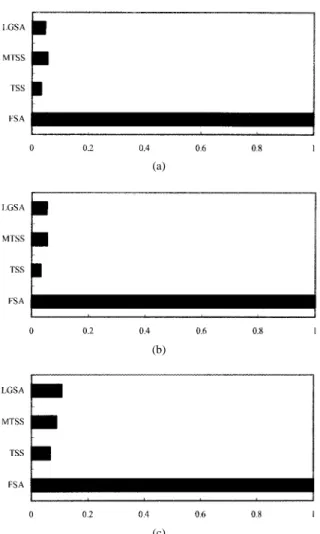
Comparisons of the block-matching numbers in different algorithms are shown in Fig. 4(a). When the overheads of genetic operations (reproduction, mutation, survival compe-tition, etc.) are taken into account, the computational cost of LGSA increases a little. Fig. 4(b) shows the ratio diagram of the average execution time for these algorithms. All of the algorithms are run on a SUN SPARC-10 machine. It follows from the figure that LGSA needs more computations than TSS does, but it still has fairly low computational complexity as compared to FSA.
1MPEG-1 video software encoder, developed by L. A. Rowe, K. Gong,
K. Patel, and D. Wallach, Computer Science Division—EECS, University of California at Berkeley.
(b)
(c)
Fig. 4. Comparisons of the computational complexity ratio: (a) average block-matching numbers, (b) average execution time of separated BMA’s, and (c) average execution time of MPEG encoders using different BMA’s.
When the search algorithms are embedded into the MPEG encoder, it is important to inspect the computational complex-ity of the whole system. Fig. 4(c) shows the ratio diagram of the average encoding time for one video frame by using different block-matching algorithms. The computational com-plexity of the encoding system is largely reduced when fast search algorithms are applied. Although the original execution time of LGSA is less than MTSS, the whole execution time is more than that of MTSS while they are incorporated into the MPEG encoder. The reason is that the encoder takes more computations to decide on the type of macroblocks when the quality of the predicted image is better. However, the execution time of the system using LGSA is still very close to the other systems using TSS and MTSS, but the compression ratio is greatly improved.
proposed LGSA is under control, which is close to that of TSS and MTSS, and is much lower than that of FSA. Therefore, it is suitable to be applied in video coding systems. The proposed LGSA can be treated as an expansion of TSS, and by observing the experimental results, one can conclude that the performance of LGSA is much better than that of TSS.
In order to improve the performance of block matching, the block-matching number should be increased. However, the efficiency of the block-matching algorithm is also an important issue. MTSS improves the performance of TSS by increasing the block-matching number. In this paper, the proposed LGSA needs a similar block-matching number to MTSS, but the performance is even better.
ACKNOWLEDGMENT
The authors would like to thank the anonymous reviewers for many helpful comments and suggestions.
REFERENCES
[1] J. R. Jain and A. K. Jain, “Displacement measurement and its application in interframe image coding,” IEEE Trans. Commun., vol. COM-29, pp. 1799–1808, Dec. 1981.
[2] T. Koga, K. Iinuma, A. Hirano, Y. Iijima, and T. Ishiguro, “Motion compensated interframe coding for video conferencing,” in Proc. Nat. Telecommun. Conf., New Orleans, LA, Nov. 1981, pp. 5.3.1–5.3.5. [3] S. Kappagantula and K. R. Rao, “Motion compensated interframe image
prediction,” IEEE Trans. Commun., vol. COM-33, pp. 1011–1015, Sept. 1985.
[4] R. Srinivasan and K. R. Rao, “Predictive coding based on efficient motion estimation,” IEEE Trans. Commun., vol. COM-33, pp. 888–895, Aug. 1985.
[5] H.-M. Jong, L.-G. Chen, and T.-D. Chiueh, “Accuracy improvement and cost reduction of 3-step search block matching algorithm for video coding,” IEEE Trans. Circuits Syst. Video Technol., vol. 4, pp. 88–90, Feb. 1994.
[6] K. H.-K. Chow and M. L. Liou, “Genetic motion search algorithm for video compression,” IEEE Trans. Circuits Syst. Video Technol., vol. 3, pp. 440–445, Dec. 1993.
[7] I. K. Kim and R.-H. Park, “Block matching algorithm using a genetic algorithm,” in SPIE Symp. Visual Commun. Image Processing, Taipei, Taiwan, May 1995, pp. 1545–1552.
[8] D. E. Goldberg, Genetic Algorithms in Search, Optimization & Machine Learning. Reading, MA: Addison-Wesley, 1989.
[9] J. L. R. Filho and P. C. Treleaven, “Genetic-algorithm programming environments,” IEEE Comput. Mag., pp. 28–43, June 1994.