International Journal of Sediment Research, Vol. 17, No. 3, 2002, pp. 197-210 - 197 -
MODELING THE FATE AND TRANSPORT
OF HYDROPHOBIC ORGANIC COMPOUNDS IN
AN UNSTEADY RIVER-ESTUARINE SYSTEM
Su-Chin CHEN1 and Jan-Tai KUO2
ABSTRACT
This research develops a generalized, one-dimensional, finite difference model for simulating the distribution of toxic substances in a river-estuarine system. The three sub-models for unsteady flow, sediment transport, and the reaction of toxic substances are also presented using an uncoupled numerical method. The paper also includes experimental work for sorption/desorption, field measurements of organic carbon content in the heavily polluted Keelung River, and a laboratory study of cohesive sediment transport for the model calibration and verification. In addition, this study simulates the polycyclic aromatic hydrocarbons (PAHs) in the Keelung River in northern Taiwan as a case study. Encouraging results are obtained, and suggest that the modeling approach could be extended to simulate the fate and transport of sorbed pollutants in tidal river.
Key Words: Toxic substance model, Tidal flow, Sediment transport, Sorption and desorption kinetics, Polycyclic Aromatic Hydrocarbons (PAHs), Keelung River
1 INTRODUCTION
Extensive literature (Brown et al., 1985; Sawhney et al., 1981; Bierman and Swain, 1982; Connolly, 1980; Lopez-Avila and Hites, 1980; O’Connor, 1988) described lots of sorbed pollutants or toxic substances in bed sediments of rivers, even after the effluent was halted for a long time. This is particularly true for hydrophobic organic compounds that can be sorbed on the particles and accumulated in the river bed sediments (Karickhoff et al., 1979). Pollution events of highly sorbed toxic substances have been reported for several years, e.g. polychlorinated biphenyls (PCBs) in the Hudson River, New York, (Brown et al., 1985; Turk, 1980; Bopp et al., 1981) and the pesticide kepone in the James River, Virginia (Huggett etal., et al., 1980). The U.S. Environmental Protection Agency (EPA) lists 129 priority pollutants that represent the most common co nditions. It should be noted that chemical becomes toxic substance when beyond a certain concentration, it has a harmful impact.
Toxic substances have been found in rivers in Taiwan, such as polycyclic aromatic hydrocarbons (PAHs) in bed sediments of the Keelung River (Kuo et al., 1990). This research develops a model for simulating the distribution of toxic substances in rivers, focusing on the fate and transport of hydrophobic organic compounds such as polycyclic aromatic hydrocarbons (PAHs) in the tidal river.
Three parts comprise this research. First, sediment samples taken from the Keelung River were analyzed for stress of cohesive sediments and size distribution of sediments. From water samples, the concentrations of PAHs were analyzed using a gas chromatograph (GC) (Kuo et al., 1990). Second, three numerical sub-models were developed for unsteady state hydraulics, sediment transport, and the fate of toxic substances. Third, model calibration for the parameters (e.g. Manning’s n and dispersion coefficient E, etc.) and model validation for simulating distribution of PAHs in the Keelung River were performed (Chen, 1990).
This paper discusses numerical methods for the model used, the interaction among these three sub-models, and their application results. The models may be used to simulate hydrophobic organic compounds in a
1
Professor, Department of Soil and Water Conservation, National Chung-Hsing University, Taichung, 402,Taiwan, China, E-mail: scchen@dragon.nchu.edu.tw
2
Professor, Department of Civil Engineering, National Taiwan University, Taipei, 106, Taiwan, China Note: The manuscript of this paper was received in July 2001. The revisd version was received in April 2002. Discussion open until Sept. 2003.
river-estuarine system to provide both a better understanding of and an effective tool for managing water quality and assessing the environmental risk of toxic substances.
2 MODEL FRAMEWORK AND EQUATIONS
The fate of hydrophobic organic compounds in a tidal river or estuary is more complex than in a non-tidal river. Not only the three T’s, transport, transfer, and transformation influence the fate of toxic substance, but also hydrodynamics (advection and dispersion), biochemical reaction, sorption/desorption, and sediment transport. Most models cannot adequately simulate the fate of hydrophobic organic compounds and the distribution of sediments in an unsteady tidal river network. For example, EXAMS (Burns et al., 1981) only simulates the contaminant transport in steady flow and is not designed to simulate toxic substance concentrations in a tidal river. Also, the dispersion term is not considered in the SERATRA (Onishi and Wise, 1979) model; it can only be used to model toxic substances in a nontidal river in which the effect of advection is much larger than that of dispersion. TOXIWASP (Ambrose et al., 1983) considers only one size of sediment using a simple simulation of the actual river system that does not consider the sorbability of toxic substances as a function of particle size. This research develops a more generalized model that simulates the fate of hydrophobic organic compounds in a tidal river network. To decrease computation, the model uses an uncoupled numerical approach. Flow continuity and momentum equations are first solved. The solutions yield the discharge, water depth, and velocity etc., which are then used in sediment transport equations that consider the bed load and suspended load transport. Finally, results from sediment concentrations are substituted into toxic substance transport equations to resolve the fate of hydrophobic organic compounds in the river flow and bed, respectively. The detailed framework of the governing equations and the numerical schemes are described as follows.
2.1 Hydraulic Sub-model
The mechanism of sediment transport and the flow condition influence the fate of hydrophobic organic compounds in a natural water body. Flows are generally unsteady in a tidal river (such as the Tanshui River) that receives tributary inflows and is influenced by tidal fluctuation. This causes pollutant concentrations in the water body also to be unsteady. An unsteady water-quality model is usually required to accurately simulate distribution of contaminant concentrations. Results of an unsteady hydraulic model can provide detailed hydraulic information for the sediment transport and toxic substance sub-models. The Saint Venant equations for unsteady flow in one-dimensional rivers can be represented as the continuity equation
l q x Q t A+ = ∂ ∂ ∂ ∂ (1)
and the momentum equation
l l f qV S S gA x y gA A Q x t Q+ + = − + ) ( ) ( 0 2 ∂ ∂ ∂ ∂ ∂ ∂ (2)
where Q = discharge in x direction, A = area of the cross-section, ql = lateral inflow per unit length, Vl =
velocity component in x direction from the lateral inflow, S0 = river bed slope, Sf = friction slope =
n2Q|Q|/A2R4/3, R = hydraulic radius, n = Manning’s roughness coefficient, t = time, y = water depth, and g =
acceleration of gravity.
Equations 1 and 2 represent a set of hyperbolic partial difference equations for which analytic solutions do not exist for a natural water body. The linear Preissmann fully implicit scheme of finite difference method (Mahmood and Yevjevich, 1975; Liggett and Cunge, 1975) is used to solve Q and A (or y) in equations (1) and (2).
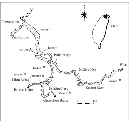
The number of junctions in the river network depends on the number of tributaries and the type of river network, e.g. two junctions in the Tanshui River network. The simulative framework for toxicants in Tanshui river-estuarine system is illustrated in Fig. 1. Keelung River, Taham Creek and Hsintien Creek are the three tributaries of Tanshui River. For the low elevation in the Taipei Basin, the movement of the tide into and out of the Tanshui River network that we simulated in the study. At each river junction, such as Hsintien Creek merged into Taham Creek, junction B, and Keelung River merged into Tanshui, junction A, we assume a small value for A(dy/dx) (where y is the average water depth at the junction) and negligible velocity head differences among three cross-sections for each junction. Then, the discharges and water depths can be calculated through a junction from upstream to downstream.
International Journal of Sediment Research, Vol. 17, No. 3, 2002, pp. 197-210 - 199 - Kuantu Peilin Bridge Hsintien Creek Chungcheng Bridge Taiwan Strait R e a c h ⒒ junction B R e a c h ⒐ Hsinhai Bridge Taham Creek Tanshui River junction A R e a c h ⒔ Keelung River Nanfu Bridge R e a c h ⒑ 0 4Km N Wutu R e a c h ⒓ Taiwan
Fig. 1 Segmentation for the finite difference model of Tanshui Tidal River Network 2.2 Sediment Sub-model
The partition coefficient and sediment load determine the fraction of a pollutant sorbed on particulate solids. Predicting the transport and fate of sorbed pollutants requires understanding the behavior of particles in the water body. Predicting particle behavior is, however, difficult and uncertain in water-quality modeling. Much available knowledge pertains to large particles controlling the stream configuration rather than to small particles that adsorb lots of the toxic pollutants.
Bed sediments consist of gravel, sand, and silt and are classified as non-cohesive sediments in upstream Keelung River. Downstream sediments consist of silt, clay, and organic matter and are classified as cohesive sediments. The hydrodynamic behavior of fine cohesive sediments in a turbulent flow field is more complex and less understood than that of coarse sediments. Non-cohesive sediment beds resist erosion by the submerged weight of individual grains, which provide mutual support by friction (Partheniades, 1965). By contrast, cohesive sediments consist of particles sufficiently small and with a sufficient surface-to-mass ratio that their surface physico-chemical forces are much more important than their weight.
The transport of cohesive sediments has been studied using the statistical model (Partheniades, 1972), three-dimensional transport model (Nicholson and O’Connor, 1986), the two dimensional transport model (Onishi and Wise, 1979), and the one-dimensional transport model (Scarlatos, 1981). Most of these models consider only one sediment size without considering non-uniform sizes that exist in a nature river. Further, they consider only steady state river flow without including the tidal current in an estuary. The sediment model developed herein considers suspended sediments, bed sediments, and four different sizes of sediment in each part. This sediment model simulates transporting of multisize sediments in a river and estuary network. Such a measure is needed to accurately model toxic substances, because the sorbability of toxic substances is a function of particle sizes.
To understand the property of cohesive sediment in the river bed for the downstream portion of the Keelung River, samples were taken for a viscous test using a rotated cylinder tensor meter. Experimental results showed the yield stress of bed sediment in the Keelung River at about 300 dyne/cm2. However, the shear stresses in normal discharge are less than 20 dyne/cm2 in the Keelung River. Since the bed load cannot be
sediment concentrations of river bed Sb remain constant at normal discharge, implying that the ∂ Sb/∂ t is
equal 0 (steady) but ∂ Sb/∂ x is not equal 0 (non-uniform) in the bed sediment equation.
The net particle flux across the bed-water interface can be expressed as the difference between the deposition (settling) flux and the erosion (resuspension) flux. The deposition flux is related to the settling velocity, Ws, and the concentration of solids in the water column, Sw. The erosion flux is related to the
resuspension velocity, Wrs, and the concentration of solids in the river bed, Sb. However, the Ws and Wrs
depend on the shear stress τ. If τ is less than the critical deposition shear stress, τD, deposition will occur. On
the other hand, if τ exceeds the critical erosion shear stress, τE, erosion happens. If τ ranges between τE and τD
that is τE >τ> τD, the scouring is equal deposition.
The mass balance equations of suspended sediments is given by
V W S y W S y W x S U x S E t S psi i b i rs E i w i s D i w i w i w , , , , , , 2 , 2 , ) 1 ( ) 1 ( − + − + − − = τ τ τ τ ∂ ∂ ∂ ∂ ∂ ∂ (3)
and the continuity equation for bed sediments is
i w i s D i b i b i rs E S W S W W , ,] , (1 ) , , ) 1 [( τ τ τ τ − + = − (4)
where i=1,2,3,4 represents four different sediment sizes, s D W ) 1 ( τ τ
− = effective settling velocity, rs E W ) 1 ( − τ τ
= effective resuspension velocity, 0<(1− )<1
D
τ
τ = the rate of deposition ranging between 0 and 1,
) 1 ( 0< − E τ
τ = the rate of resuspention and exceeds 0, E = longitudinal dispersion coefficient (assuming that E is a function of flow velocity U and hydraulic depth R), Wps = sediment input loading per unit time from
lateral flow, Wb = sedimentation velocity from active bed sediment layer to deep bed sediment layer, V =
volume of water column, and the subscript of w,b represent water column and bed sediment, respectively. Each sediment of different size is assumed here to be fully mixed in the river bed. Therefore, τD and τE are
independent on the sediment size in this model, but Wrs,i and Ws,i are functions of sediment size, and the
sediment size still affects effective settling velocity si D W, ) 1 ( τ τ
− and effective resuspension velocity
i rs E W , ) 1 ( − τ τ .
Since Sb,i is constant in every river segments but different between each others, Sw,i can be directly solved
from equation (3). Substituting the solution of Sw,i into equation 4, the sedimentation velocity Wb,i for each
size of sediment can be known. If Wb,i is positive, there is deposition or, otherwise, erosion. By repeating
these processes, the concentration of each sediment size in the water column and river bed can be solved from equations (3) and (4). The information can then be used to solve the total concentrations of hydrophobic organic compounds in the river flow and bed sediments. Equation (3) is an advection-dispersion transport equation so the Crank-Nicolson implicit scheme (Smith, 1978) of a finite difference method is used to solve the sediment concentration.
2.3 Toxic Substance Sub-model
Factors influencing the concentration of toxicants in a river-estuarine system include: (a) transporting of the toxicant due to advection and dispersion, (b) decay by irreversible chemical transformations, (c) partitioning of toxicant between dissolved and particulate phases in both the river flow and bed sediments, (d) settling and resuspension mechanisms of particles, (e) diffusive exchange between the river flow and the bed layer, and (f) net deposition and loss of a chemical to deep sediments.
The toxicant can exist in two basic forms: the toxicant in the dissolved phase, Cd , and the toxicant on the
solids, Cp, both in the river flow or bed sediment (Thomann and Mueller, 1987). The toxicant can be
selectively sorbed onto certain types of solids, such as finely dispersed clays or organic particles. Consequently, four categories of sediments are considered here. The total toxicant concentration CT in the
International Journal of Sediment Research, Vol. 17, No. 3, 2002, pp. 197-210 - 201 - The particulate form, Cp, is expressed as a mass of toxicant per bulk volume of solids and water. A given
concentration of solids S, Cp can also be expressed as Cp = γpS, where γp denotes the toxicant concentration
expressed on a dry weight solids basis. Assuming that the sorption is reversible and that the sorption-desorption kinetics are linear part of the Langmuir isotherm (Weber, 1972), then a partition coefficient, Kπ , can be defined as
S C C C K d p d p = =γ
π (Mingelgrin and Gerstl, 1983).
Hydrophobic organic compounds are transported in either river flow or bed sediments. However, for simplification, a total concentration is used to develop the equations as follow.
Transport equation for the toxicant CTw in river flow is
Tw pw s D dw Ew Tw Tw Tw Tw C f y W f K K x C E x C U t C ] ) 1 ( [ 2 2 τ τ ∂ ∂ ∂ ∂ ∂ ∂ + = − + + − Tb pb rs E db Ew f C y W f K ( 1) ] [ + − + τ τ φ Tw Tb Tw C C x C E −Ψ +Ω = 2 2 ∂ ∂ (5)
and transport equation for the toxicant CTb in bed layer is
Tb pb b b pb rs E db Eb Tb Tb C f y W f y W f K K t C ] ) 1 ( [ + + − + − = τ τ φ ∂ ∂ pw Tw Tb Tw b s D dw Eb f C C C y W f K + − =−Θ +Φ +[ (1 ) ] τ τ (6) in which pw s D dw Ew Tw f y W f K K (1 ) τ τ − + + = Ψ pb rs E db Ew f y W f K +( −1) = Ω τ τ φ pb b b pb rs E db Eb Tb f y W f y W f K K + + − + = Θ ( 1) τ τ φ pw b s D dw Eb f y W f K (1 ) τ τ − + = Φ
where yb = depth of active bed sediments, CTw = total concentration in water body, CTb = total concentration
in bed sediments, KT = decay coefficient, KE = Ev/ly =vertical diffusion rate between water body and active
bed sediment layer, Ev = vertical diffusion coefficient, l = character length, φ = porosity of bed sediment.
In the above equations, fpw , fdw , fpb , and fdb represent the fractions of toxicant concentration in the river
flow and bed sediment, respectively. The relation between CT and Cd is CT =Cd+KπSCd =(1+KπS)Cd, so
the equations yield as follow
∑
∑
= = + = 4 1 , , 4 1 , , 1 i i w i w i i w i w pw S K S K f π π∑
= + = 4 1 , , 1 1 i i w i w dw S K f π∑
∑
= = + = 4 1 , , 4 1 , , 1 i i b i b i i b i b pb S K S K f π π∑
= + = 4 1 , , 1 1 i i b i b db S K f π (7)That is, Cdw = fdw CTw , Cpw = fpw CTw as well as Cdb = fdb CTb , Cpb = fpb CTb, where fdw and fpw are dissolved
fraction and particulate fraction in the water body, respectively. As equation 7 indicates, fdw + fpw =1.0 and
sediment. From equations 5 and 6, CTw and CTb can be solved. Then, the dissolved and particulate
concentrations can be obtained using the partition coefficient. An octanol/water partition coefficient Kow
often is used to calculate the sediment sorption coefficient based on organic carbon content Koc, then, from
the percentage of organic carbon in sediment foc, Kπcan be calculated (Lyman et al., 1982).
Since the equation of sediment transport is similar to those of the fate of toxic substances in form, the numerical methods of Crank-Nicolson implicit difference scheme was also applied for equations 5 and 6. If we combine the above six equations (equations 1and 2; equations 3 and 4; equations 5 and 6), it would produce an enormous matrix for the implicit finite difference scheme requiring much more time for calculations. Therefore, the uncoupled method was chosen. First, from unsteady flow equations (equations 1 and 2), the discharge, velocity, and water depth can be obtained for every time step and at each segment. Substituting those hydraulic variables into the sediment transport equations (equations 3 and 4) yields the concentrations of suspended sediments and bed sediments. Finally, the hydraulics and sediment concentrations are substituted into the transport equations of hydrophobic organic compounds (equations 5 and 6). Accordingly, the total toxic substance concentration can be solved in each river flow and bed layer. 3 MODELING PAHS IN KEELUNG RIVER
Above models were applied to the Tanshui River system (Fig. 1) located in northern Taiwan. The Tanshui River is a major river-estuarine that flows through Taipei. The watershed for the entire Tanshui River basin is about 2,700 km2. The low portion of this river is severely polluted by municipal and industrial waste discharges. During low flow, dissolved oxygen concentrations in some portions of the river can be zero. Sanitary sewers and wastewater treatment plants are in planning stages or under construction in Taipei, while in Taipei County, the construction of a huge regional wastewater treatment plant for ocean outface has just been completed to reduce the polluting of the Tanshui River.
Taham Creek, Hsintien Creek and the Keelung River are three major tributaries of the Tanshui River system. Fig. 1 represents the portion of the river system under this study, consisting of five reaches (I to V) and two junctions. Each reach is further divided into some segments. The river system under study is unsteady in both hydrodynamics and water quality because of tidal effects.
Without available data for toxic substances in the main Tanshui River, this study simulated the distribution of toxic substances (polycyclic aromatic hydrocarbons, or PAHs) in the Keelung River tributary that joins Tanshui River at Kuantu. For the hydraulics model, however, it was applied to the entire Tanshui River system. No station measure track water level at Kuantu, so hydraulic data lack downstream boundary conditions for the Keelung River hydraulic modeling. The problem can be resolved by modeling hydraulics for the entire Tanshui River system with the available downstream water level boundary conditions at the mouth of theTanshui River, as well as three upstream discharge boundary conditions at Wutu (Keelung River), Hsinhai Bridge (Tahan Creek), and Chungcheng Bridge (Hsintien Creek).
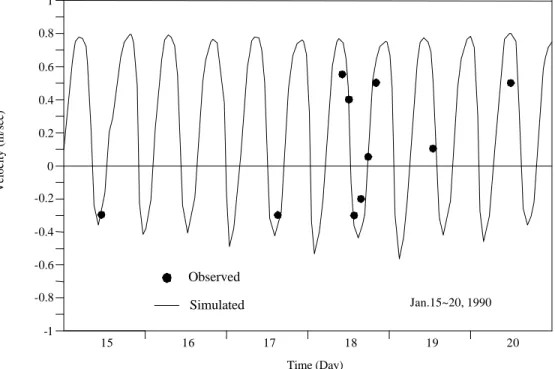
Natural channel cross-sections were replaced by more regular shaped cross-sections favorable for computation. Values of Manning’s n were determined from hydraulic model calibration by comparing computed Q and y to measured data. The values of Manning’s n from upstream Wutu to downstream Kuantu were found in the range from 0.025 to 0.015 in the Keelung River. The Manning’s n at upstream are greater than those at downstream because the upstream bed sediments are more coarse. Verification of the hydraulic model was consecutively performed and showed favorable results. Fig. 2 displays a kind of type of the hydrodynamic model simulation and its comparison to the measured field data at Nanfu Bridge in Keelung River. As this figure reveals, the tidal current variation between 0.7 m/sec (ebb, downstream direction) and -0.3m/sec (flood, upstream direction) during January 15-20, 1990, at Nanfu Bridge.
International Journal of Sediment Research, Vol. 17, No. 3, 2002, pp. 197-210 - 203 - -1 -0.8 -0.6 15 Velocity (m/sec) 0.2 -0.4 -0.2 0 0.6 0.4 0.8 1 Jan.15~20, 1990 Time (Day) 16 17 18 19 20 Observed Simulated
Fig. 2 Comparison of numerical results and observed data for tidal current velocity at Nanfu Bridge in Keelung River
For the dispersion coefficient E, assume that it is a function of flow velocity U and hydraulic depth R i.e.
E=CE⋅|U|⋅R, where CE is calibrated and verified using the field data of salinity. Fig. 3 presents one case of
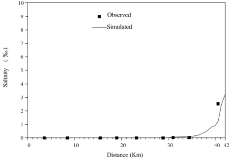
model result in dispersion coefficients and salinity concentrations at Peilin Bridge. Since E is proportional to the absolute value of flow velocity, the dispersion coefficients have two cycles every day and varies from 25 km2/day during ebb to 3 km2/day during flood at Peilin Bridge.However, dispersion coefficient is not function of time only, but function of space. In other words, dispersion coefficient has differently varied value within each segment. Further, salinity significantly varies in the reach of a tidal river, e.g. about 50
00 during flood and less than 0.10
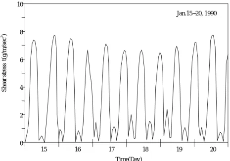
00 during ebb at Peilin Bridge. Figs. 4 and 5 show the low water slack and high water slack profiles for salinity from Wutu (upstream) to Kuantu (downstream) in Keelung River. As seen, a translation of the salinity results from the tidal oscillation. However, the salinity have not penetrated to the Peilin Bridge, the location at 30km in Fig. 4, so that the tidal river is still ‘fresh’ after Peilin Bridge. Sediment sizes in the Keelung River were surveyed in each of its segments. Four sediment sizes, D1= 1.0 mm, D2=0.1 mm, D3=0.02 mm, and D4=0.006 mm, were chosen for the model. Field data shows different percentages of each sediment size in every river segments (Chen, 1990). The water level oscillations were known at Kuantu from simulation of hydraulics for the whole Tanshui River system. Therefore, the sediment transport modeling was carried out in the Keelung River from upstream Wutu to Kuantu only. From sediment model calibration, the critical deposition shear stress τD is 5 dynes/cm2 and critical erosion shear
stress τE is 10 dynes/cm2. Fig. 6 shows simulation results of shear stress for sediments under tidal cycles at
Nanfu Bridge. Because the speeds at the ebb period exceed those at the flood period (Fig. 2), the shear stress, near 8 dynes/cm2, during ebb is larger than during flood, when it is about 1 dynes/cm2. This is why most erosion happens during ebb and deposition happens during flood in the Keelung River. However, those shear stresses are far less than the yield stress (300 dynes/cm2) in the Keelung River. Bed sediment, then, cannot move like a plastic fluid, but instead is transported by erosion and resuspension.
Observed Simulated 1 0 3 Salinity ( ) 2 4 6 Dispersion coeffi cient (km 2/day) 40 0 20 Nov. 10, 1988 Time (hr) 5 7 9 11 13 15 17 19 21 23
Fig. 3 Comparison of numerical results and observed data for dispersion coefficient and salinity variation due to tidal current at Peilin Bridge
0 0 1 2 3 Salinity ( ) 4 5 7 6 10 9 8 Distance (Km) 10 20 30 Observed Simulated 40 42
International Journal of Sediment Research, Vol. 17, No. 3, 2002, pp. 197-210 - 205 - 0 0 1 2 Salinity ( ) 7 5 4 3 6 10 11 9 8 15 12 13 14 Distance (Km) 10 20 30 Simulated Observed 40 42
Fig. 5 Salinity distribution at high water slack tide in Keelung River
0 2 15 16 Time(Day) 17 18 19 20 Shear stress t(g/m/sec 2 ) 6 4 8 10 Jan.15~20, 1990
Fig. 6 The variation of shear stress from model output at Nanfu Bridge
Fig. 7 compares simulated suspended load with the measured data. During January 15-20, 1990, the weather was rainy. But January 18was a sunny day in which the concentration of suspended load in the river was much lower. The suspended load on rainy days was more concentrated than those on the one sunny day because sediment was washed off from the upstream hillslope. This was especially the case for January 19 and 20 in which the concentration of suspended load was between 300 and 400 mg/l. The concentrations varied in a tidal cycle due to the interaction between turbid flow from upstream and clear flow from downstream during high tide. However, the concentration of suspended sediment varied in a small range on
January 18, which, again, was a sunny day. Fig. 7 shows the accurately simulated natural phenomenon. The largest particle size D1 cannot be suspended during a normal flow so is not found in the water column. However, the second largest particle size D2 can be found during ebb, but when the shear stress is less during a flood period, it disappears. Sediment concentration D3 is also a shear-stress function, except the particle size is smaller than D2, so it is varied in a tidal cycle in the water column. The sediment size of D4 is even smaller, at a low shear stress, so it does not settle into the bed layer, maintaining a concentration that does not significantly vary with the tidal current. Figs. 8 and 9 show the high water slack and low water slack profiles for suspended solids in Keelung River. For the low shear stress, the suspended solid almost remained stable in the tidal river.
Observed Suspended sediment (ppm) Time (Day) 50 0 100 16 15 17 18 19 20 D1 = total concentration D2 = 0.001mm D3 = 0.0002mm D4 = 0.00006mm 250 150 200 300 350 400 Jan.15~20, 1990 Observed
Fig. 7 Simulated results of suspended sediment and their comparison to measured data at Nanfu Bridge
50 S.S. (mg/l) 10 20 10 0 30 40 0 Distance (Km) 20 30 Simulated Observed 70 80 60 100 90 42 40 Oct. 20, 1983
International Journal of Sediment Research, Vol. 17, No. 3, 2002, pp. 197-210 - 207 - 60 S.S. (mg/l) 10 0 30 10 20 50 40 0 Distance (Km) 20 30 Simulated Observed 90 80 70 100 42 40 Oct. 20, 1983
Fig. 9 Distribution of suspended solid at low water slack tide in Keelung River
Sampling of the tidal river at slack water can therefore be useful in certain cases for delineating water quality profiles in tidal rivers. It need only be remembered that a translation of the slack profile should be made to obtain an estimate of the mean tide profile which forms the basis of the preceding equations. From the Gas Chromatograph (GC) analysis for PAHs in the Keelung River, seven different species of PAHs were found in the river bed sediment: naphthalene, acenaphthene, fluorene, anthracene, fluoranthene, pyrene and benzo[a]anthracene. The concentrations of PAHs were usually more than 1 mg/l in river bed. Typically, only species of PAHs such as acenaphthene, fluorene, and anthracene existed in a water column because of the low partition coefficient, and those concentrations were far lower than that found in bed sediment. In the water column, concentrations of acenaphthene, fluorene, and anthracene were between 10 and 100 µg/l. Acenaphthene, an irritant for eyes and skin, and anthracene, a carcinogen, are two toxic substances for concern in modeling. Because each has lower partition coefficients than other PAHs, field data revealed them in the water column of the Keelung River.
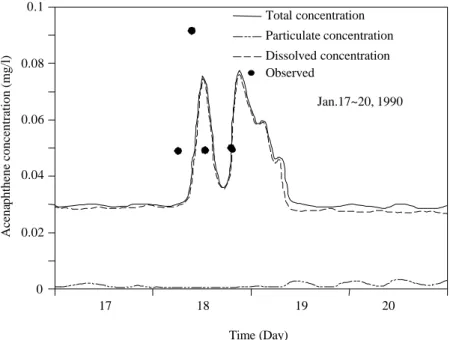
Fig. 10 compares simulated acenaphthene concentration with field data. Acenaphthene concentration created two peaks on January 18, a sunny day, because of decreased stream flow and high effluent toxicant concentration from upstream point sources. On this same day, two tidal cycles affected acenaphthene distribution. Acenaphthene concentration in the water column also depended on sediment concentration (Fig. 7). Partitioning coefficient, Kπ is low, so most acenaphthene was in its dissolved form. Suspended sediment concentration was high on January 19 and 20, so higher particulate toxicant concentration existed in the water column. Fig. 11 summarizes the simulated results of anthracene to field data, which shows influencing factors similar acenaphthene.
From the above analyses and discussions, we can conclude that these models are highly effective tools for modeling and predicting the hydraulics, sediment transport, and fate of toxic substances in a river-estuarine system.
4 CONCLUSIONS
This study simulated the distribution of toxic substances in the tidally affected Tanshui River system, particularly focusing on one of its major tributaries, the Keelung River, where the field survey and sampling analysis were done. Field data include river geomorphology, tidal current hydraulics, suspended sediment, and bed sediment property, as well as toxic substance sampling analysis. The Keelung River receives significant municipal and industrial waste effluents and is a seriously polluted, tidally affected river. Field data reveals that cohesive sediment existed in the downstream river bed and that kinds of toxic substances were sorbed in a river bed that was more seriously contaminated than the water column. Removing the hydrophobic organic compounds from the river bed in a normal condition is extremely difficult.
Acena p h th ene concentration (mg/l) 0 17 0.02 0.04 0.06 0.08 0.1 Dissolved concentration Jan.17~20, 1990 Time (Day) 18 19 Observed 20 Total concentration Particulate concentration
Fig. 10 Comparison of simulated acenaphthene concentration with field data at Nanfu Bridge
Anthracene concentration (mg/l) 0 0.1 17 0.3 0.2 0.4 Jan.17~20, 1990 Particulate concentration Dissolved concentration Time (Day) 18 19 Observed 20 0.5 Total concentration
International Journal of Sediment Research, Vol. 17, No. 3, 2002, pp. 197-210 - 209 - This research developed a one-dimensional, finite-difference, finite-segment, river-network model, capable of simulating the tidal current, sediment transport, and fate of hydrophobic toxic substances. The models require parameters such as Manning’s n, dispersion coefficient, and critical shear stress for calibration and validation. First, for the unsteady hydraulic sub-model, the calibrated Manning’s n ranges from 0.025 to 0.015 in the Keelung River. Second, salinity concentration, as used for the constituent transport equation, shows the calibrated and verified real-time dispersion coefficient E depends on flow velocity and water depth. Third, comparing simulated sediment concentration with the field data revealed the critical deposition shear stressand critical erosion shear stress. Finally, encouraging simulated results of PAHs concentration were obtained by comparing them with available field data. Our results indicate that the feasible numerical model can simulate the hydraulic conditions, sediment, and toxicants in a river-estuarine system and will prove a favorable tool for water pollution control.
ACKNOWLEDGEMENT
This research work was supported by National Science Council, Taiwan under project No. NSC-77-0410-E002-27, NSC -78-0421-E002-17Z, and NSC-79-0421-E002-29Z.
REFERENCES
Ambrose, R. B., Hill, S. I. and Mulkey, L. A. 1983, User's Manual for the Chemical Transport and Fate Model TOXIWASP, U.S. EPA Environmental Research Laboratory, Athens, Georgia.
Bierman, J. V. J. and Swain, W. R. 1982, Mass balance modeling of DDT dynamics in lakes michigan and superior. Environ. Sci. & Technol., Vol. 16, pp. 572-579.
Bopp, R. F., Simpson, H. J., Olsen, C. R. and Kostyk, N. 1981, Polyclhlorinated biphebnyls in sediments of the tidal Hudson River, New York. Environ. Sci. & Technol., Vol. 15, pp. 210-216.
Brown, M. P., Werner, M. B., Sloan, R. J. and Simpson, K. W. 1985, Polychlorinated Biphebnyls in the Hudson River. Environ. Sci. & Technol., Vol. 19, pp. 656-661.
Burns, L. A., Cline, D. M. and Lassiter, R. R. 1981, Exposure Analysis Modeling System (EXAMS) User Mannual and System Documentation, US EPA Environmental Research Laboratory, Athens, Georgia.
Chen, S. C. 1990, Modeling the Fate of Hydrophobic Organic Compounds in a Dynamic River-Estuarine System, Ph.D. Dissertation, National Taiwan University, Dept. of Civil Eng., Taiwan (in Chinese).
Connolly, J. P. 1980, The Effect of Sediment Suspension on Adsorption and Fate of Kepone, Univ. of Texas in Austin, Ph.D. Dissertation.
Huggett, R. J., Nichols, M. M. and Bender, M. E. 1980, Kepone contamination of the James River Estuary. Contaminants and Sediments, Vol. 1, Edited by R.A. Baker, Ann Arbor Science, Ann Arbor, MI, pp. 33-52.
Karickhoff, S. W., Brown, D. S. and Scott, T. A. 1979, Sorption of hydrophobic pollutants on natural sediments. Water Research, Vol. 13, pp. 241-248.
Kuo, J. T., Wu, S. C. and Chen, S. C. 1990, Modeling Toxic Substances in Rivers, Report No. NSC 79-0421-E002-29Z, Dept. of Civil Engineering, National Taiwan University, Taipei, Taiwan (in Chinese).
Liggett, J. A. and Cunge, J. A. 1975, Numerical methods of solution of the unsteady flow equation. Chapter 4 in Mahmood, K. and Yevjevich, V. (editors), Unsteady Flow in Open Channel, Vol.1, Water Resources Publications, Fort Collins, Colorado, pp. 1663-1678.
Lopez-Avila, V., and Hites, R. A. 1980, Organic compounds in an industrial wastewater. their transport into sediments. Environ. Sci. & Technol., Vol. 14, pp. 1382-1390.
Lyman, W. J., Reehl, W. F. and Rosenblatt, D. H. 1982, Handbook of Chemical Property Estimation Methods, McGraw-Hill, Inc..
Mahmood, K., and Yevjevich, V. 1975, Unsteady Flow in Open Channels, Vol. 1, Water Resources Publications Inc., Fort Collins, Colorado.
Mingelgrin, U., and Gerstl, Z. 1983, Revaluation of partitioning as a mechanism of nonionic chemical adsorption in soils. J. Enviro. Qual., Vol. 12, pp. 1-11.
Nicholson, J. and O'Connor, B. A. 1986, Cohesive sediment transport model. J. of Hydraulic Eng., ASCE, Vol. 112, pp. 621-640.
O’Connor, D.J. 1988, Models of sorptive toxic substances in freshwater systems III: streams and rivers. J. of Environmental Engineering, ASCE, Vol. 114, pp. 552-574.
Onishi, Y. and Wise, S. E. 1979, Mathematical Model, SERATRA, for Sediment Contaminant Transport in Rivers and its Application to Pesticide Transport in Four Mile and Wolf Creek in Iowa, submitted to US EPA, Environmental Research Laboratory at Athens, GA. by Battle Pacific Northwest Laboratories, Richland, WA.
Partheniades, E. 1972, Results of recent investigations on erosion and deposition of cohesive sediments. Sediment, Chap.20, H. W. Shen (ed.)
Sawhney, B. L., Frink, C. R. and Glowa, W. 1981, PCBs in the Housatonic River : determination and distribution. J. Environ. Qual., Vol. 10, pp. 444-448.
Scarlatos, P. D. 1981, On the numerical modeling of cohesive sediment transport. J. of Hydraulic Research, Vol. 19, pp. 61-68.
Smith, G. D. 1978, Numerical Solution of Partical Differential Equationl, Clarendor Press, Oxford.
Thomann, R. V. and Mueller, J. A. 1987, Principles of Surface Water Quality Modeling and Control, Chapter 8, Harper & Row Publishers, New York.
Turk, J. T. 1980, Application of Hudson River Basin PCB-transport studies, Contaminants and Sediments, Vol. 1, Edited by R.A., Baker, Ann Arbor Science, Ann Arbor, MI, pp. 171-183.
Weber, W. J. 1972, Physicochemical Processes for Water Quality Control, John Wiley & Sons, New York. NOTATION
A = = area of the ross-section;
Cd = the toxicant in the dissolved phase;
Cp = the toxicant on the solids Cp = γpS;
CT = total toxicant concentration;
Ev = vertical diffusion coefficient;
KE = vertical diffusion rate between water column and active bed sediment layer;
KT = decay coefficient;
Kπ = partition coefficient, Kπ=γp/Cd=Cp/(CdS);
n = Manning’s roughness coefficient;
fpw , fdw , fpb , fdb = the fractions of toxicant concentration in the water column and bed sediment, respectively;
g = acceleration of gravity;
ql = lateral inflow per unit length;
Q = Discharge;
R = hydraulic radius;
Sb = sediment concentrations of river bed;
Sf = friction slope = n2Q|Q|/A 2
R4/3;
S0 = river bed slope;
Sw = concentration of solids in the water column;
Ub = velocity of bed sediment layer;
Vl = velocity component in x direction for the lateral inflow;
Wps = sediment input loading per unit time from lateral flow;
Wrs = resuspension velocity;
Ws = settling velocity;
yb = depth of active bed sediment;
γp = the toxicant concentration expressed on a dry weight solids basis;
φ = porosity of bed sediment;
τ = shear stress;
τD = critical deposition shear stress;