NUMERICAL SIMULATIONS OF SCOUR AND
DEPOSITION IN A CHANNEL NETWORK
Hong-Yuan LEE1 and Hui-Ming HSIEH2
ABSTRACT
A numerical model, which is capable of simulating scouring and deposition behaviors in a channel network, is developed in this study. The model treats suspended load and bed load separately, and hence is able to simulate the depositional behavior of the suspended sediment under a nonequilibrium process. The model solves the de Saint Venant equation, and thus can be applied to unsteady flow conditions. An internal boundary condition based on the sediment transport capacity was proposed to distribute the incoming sediment load into the downstream links. An assessment of this model's performance has been conducted through a comparison to an analytical solution. The application of this model to the Tanhsui River system in Taiwan, and several hydraulic model studies gave very convincing results.
1 INTRODUCTION
Evolution of the river bed in alluvial channels has been studied by many researchers using analytical and numerical approaches. The use of analytical approach alone is insufficient for solving natural river engineering problems. With rapid growth in computer technology, numerical models have become a popular means for the study of mobile bed hydraulics.
During the past decade, several numerical models have been developed. Most of the computer codes, such as HEC2SR (Simons & Li Assoc. Inc., 1980), FLUVIAL-12(Chang &Hill, 1976), HEC6 (Thomas & Prashum, 1977), IALLUVIAL (Karim & Kennedy,1982), SEDICOUP (Holly & Rahuel, 1990), BRALLUVIAL (Holly et al, 1985), CHARIMA (Holly et al, 1990),and ONED3X (Lai, 1987), stayed with a one-dimensional approach, and only few of them, such as TABS-2 (Thomas et al., 1985) and MOBED 2 (Spasojevic, 1988) are two-dimensional models. The BRALLUVIAL (Holly et al., 1985) and CHARIMA (Holly et al., 1990) codes were developed for simulating bed evolution of a branched and looped channel system. Both models are applicable to subcritical flow conditions, BRALLUVIAL is a quasi-steady code, and CHARIMA is an unsteady code.
Using the stream tube concept to reflect the lateral variations of the channel geometry, two quasi-two-dimensional models were developed, namely GSTARS (Molinas and Yang, 1986) and USTARS (Lee et al., 1997). The GSTARS model is a steady code and USTARS is an unsteady code.
A new model, named NETSTARS, is developed in this article to simulate the bed evolutions of a cha nnel network. It treats the suspended load and bed load separately, and hence is able to simulate the depositional behaviors of the suspended sediment under a nonequalibrium process. An internal boundary condition based on the sediment transport capacity was proposed to distribute the incoming sediment load into the downstream links. The details of the mathematical basis and numerical techniques are described in the following sections. Experimental data and analytical solution are used to assess the model's capability. The model is applied to simulate the bed evolution of the Tanhsui River system, which is an esturine channel network, and several hydraulic model studies to demonstrate its engineering applicabilities. The first is a standard tree-type river system, and the others are shown the capacity of looped-type channel network.
2 THEORETICAL BASIS AND GOVERNING EQUATIONS
The NETSTARS model is an uncoupled sediment routing model. It consists of two major parts, namely
1
Prof., Dept. of Civil Engr., National Taiwan Univ., Taipei, Taiwan, China, E-mail: d90521017@ms90.ntu.edu.tw
2
Assistant Professor, Dept. of Information Management, Diwan College of Management, Tainan , Taiwan, China. Notes: The manuscript of this paper was received in April 2002. The revised version was received in Nov. 2002.
hydraulic routing and sediment routing. Suspended load and bed load are treated separately in sediment routing. The governing equations for flow and sediment continuity are di scretized by the Preissmann four point scheme . The equation for suspended sediment movement is solved by Holly-Pressimann two-point four-order scheme, and T scheme.
A network algorithm was proposed to resolve the nodal point problem same as CHARIMA model. A node is assumed to be a virtual section that could not accumulate water and sediment, i.e. no scour and no deposition. A nodal continuity equation was proposed in this paper. Double sweep method is applied to solve the discharges and the water stages at those nodes. The allocation of the suspended load at the node is assumed to be proportional to the allocations of the flow discharges, and the net flux of the suspended sediment due to longitudinal dispersion is assumed to be zero at a nodal point.
The NETSTARS model avails some good ideas of CHARIMA and GSTARS models to develop a powerful tool for resolving the problems of unsteady sediment process in a channel network. Since it is basically a 1-D model, secondary current and local scour can not be simulated by this model, but the transverse bed evolution can be computed due to using the stream tube concept to decide the tube boundary for satisfying equal conveyance requirement across the channel and adding transverse transport term into the convection-dispersion equation of computing suspended load.
2.1 Equations for Hydraulic Routing
The de Saint Venant equations are used in the unsteady flow computation. These include a continuity equation and an one-dimensional momentum equation.
x q Q t A = + ∂ ∂ ∂ ∂
(1)
0 2 = − + + + q A Q gAS x y gA A Q x t Q f ∂ ∂ β ∂ ∂ ∂ ∂
(2) where A = channel cross-sectional area; Q = flow discharge; t = time; x = coordinate in the flow direction; q = lateral inflow/outflow discharge per unit length; α =momentum correction coefficient; g = gravitational acceleration; y= water surface elevation; S QQ/ K2
f= = friction slope; 3 / 2 1 AR n K= =
channel conveyance;
n
= roughness coefficient of Manning's formula, and R = hydraulic radius.2.2 Equations for Sediment Routing
The governing equations include a sediment continuity equation, a sediment concentration convection-dispersion equation and a bed load equation. The Rouse number W/κu* , where W =
sediment fall velocity , κ = Von Karman's constant and u* =shear velocity, is used to distinguish between
bed load and suspended load. Particles with W/κu*>5 are treated as bed load and particles with W/κ
u*≦5 are treated as suspended load. The sediment continuity equation is given as:
(1− ) +
∑
=1 + x =0 Q QC x t A p b Nsize k k t d ∂ ∂ ∂ ∂ ∂ ∂(3) where Qb= bed load transport rate and Ck= depth-averaged concentration of the suspended sediment of size fraction k . Adt= amount of sediment scouring/deposition per unit length and
p
=channel bed porosity. The bed load transport rate Qb equals to∑
= Nsize
k1Qbk. Where, Qbk is defined as the bed load transport rate of size fraction k. The concentration C is calculated using the convection-dispersion k
equation shown as:
l r z k C z hk k S x k C x Ak x Q k C x t A k C ∂ ∂ + + = + ( ) ) ( ∂ ∂ ∂ ∂ ∂ ∂ ∂ ∂
(4) where kx and kz = longitudinal and transverse dispersion coefficients, the relations k = 5.93 ux *h and
z
k = 0.23 u*h suggested by Elder (1959) were used , and Sk = source term of the suspended sediment of size fraction k. The second term of equation (4) in the left hand side is the convection term. The first,
second, and third terms of equation (4) in the right hand side are longitudinal dispersion, reaction, and transverse dispersion terms, respectively. A similar sediment continuity equation was proposed by Holly and Rahuel (1990). In their formul ation the bed-sediment exchange or resuspension is through the source term shown in equation (5). Both approaches were tested in our previous paper (Lee et al.,1997). Holly and Rahuel's equation underestimated the scouring and deposition quantities and Eq.3 rendered a much better simulation result and hence was chosen in this model.
According to Van Rijn (1984) and Holly and Rahuel (1990), the source term Sk is the combination of
deposition and resuspension, and can be expressed as:
Sk =Sek +Sdk
(5) where Sek and Skd = the amount of sediment resuspension and deposition, respectively. The amount of
sediment resuspension can be calculated by:
S
ek=
ρ
sB
tW
kβ
kC
ek(6)
where Bt = width of the channel; Wk = fall velocity of sediment of size fraction k; βk = fractional
representation of size -class k in the active bed layers; and Cek=sediment concentration in volume close to
the channel bed by using an appropriate empirical expression, which can be calculated by the equation proposed by Van Rijn (1984)
0.3 5 . 1 015 . 0 ∗ = D T a D C k t k ek
(7)
where, Dk = particle diameter of size fraction k; D* = particle parameter =
3 / 1 2 ) 1 ( 50 − v g s D ; Tk
=transport stage parameter =
2 * 2 * 2 ' * ) ( ) ( ) ( cr cr u u u −
; ν = water ki nematic viscosity; s = specific weight of sediment particle; u*′ = grain shear v elocity =
' 5 . 0 c u g
; c' = Chezy coefficient related to grain roughness = )
3 / 12 log(
18 R D90 ; R = hydraulic radius; at = reference level above bed; u*cr = critical shear
velocity.
The appearance of βk in equation (6) limits the entrainment of grains of class k to their availability in
the active layer. The amount of sediment deposition can be calculated by using the following equation (Holly and Rahuel, 1990):
Sdk =−ρsBtWkCdk
(8)
where C is the deposition concentration , which can be estimated by Lin(1984) dk k k dk C u W C [3.25 0.55ln( )] ∗ + = κ
(9) with κ = 0.4 .
The bed load transport rate Qb can be calculated using the following equation:
b t s b q B Q ρ 1 =
(10) where qb = bed load transport rate per unit width, which is calculated using Meyer-Peter and Mueller
formula (1948), and ρs = sediment density. 2.3 Armouring Scheme
Most river beds consist of grains with a broad range of size fractions. In an erosion process, fine particles are entrained more easily and the bed surface will become progressively coarser. Ultimately, an armour coat of large particles forms, and that stops further degradation. During the aggradation process, layers of sediment will be deposited on the bed surface and the bed surface will be progressively finer.
Updating the sediment composition at every time step is necessary and cr ucial to a sediment routing model. Various techniques dealing with bed composition variation have been proposed. This model adopts the sorting and armouring techniques proposed by Bennet and Nordin (1977). In that model the bed is divided into three layers, and sediment composition computation is accomplished through the use of one or two layers depending on whether scouring or deposition occurs during that particular time step. According to this procedure the thickness of the active layer is set equal to a preselected parameter, Nt,
times the geometric mean of the largest size class used in the simulation. The active layer is defined as the bed material layer that can be worked or sorted through by the action of the flowing water in the time step, t, to supply the volume of material necessary for erosion. Therefore, the parameter Nt is related to the
duration of simulation time step. The value of parameter Nt should be increased for longer time steps. For
the net deposition case, an inactive deposition layer is used. This layer is located beneath the active layer. When the deposition of a particle size fraction of certain thickness occurs, this thichness is added to the active layer. Also, an equal thickness of active layer is added to the inactive deposition layer. The size composition and the thickness of the inactive deposition layer is recomputed. Finally, the size computation of the active layer is recomputed and the channel bottom elevation is updated.
3 COMPUTATIONAL PROCEDURES
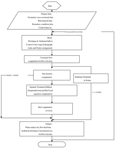
The simulation processes consist of three parts in every time step, i.e., flow computations, and sediment routing. Flow computation is performed first. Then, sediment routing is performed to calculate the amount of channel bed variations. The computational flow chart is shown in Fig. 1. These procedures are described sequentially in the folowing sections.
Start
Prepare data: Geometric cross-sectional data
Bed material data Boundary condition data
Control data etc.
Read: Discharge & Sediment Inflow Control water stage hydrograph Links and Nodes arrangement
Size fraction computation
Separate Treatment Method (Suspended load and Bed-load
equation computation)
Output: Water surface ele.,New bed form, Sediment discharge,Concentration etc.
for River System Bed computation revision
Stop
KSIZ=1,NSIZE
Do loop until the end time
Unsteady flow computation for River System
L=1,LINKS
Sediment Treatment in Nodes
3.1 Hydraulic Routing
Eqs.1 and 2 are transformed into difference equations using a Preissmann four point fi nite difference scheme. The detail terms of the difference equations had been conducted by the authors in their previous paper (Lee et al., 1997), and will not be repeated herein.
3.2 Stream Tube Computation
The algorithm for stream tube computation used for this model is the same as that of the GSTARS model developed by Molinas and Yang (1986). A literature survey has been conducted by the authors in their previous paper (Lee et al., 1997), and will not be repeated herein.
3.3 Sediment Routing
The difference equation for the sediment continuity equation, i.e., equation (3), is shown as:
( )(
)
2 / ) ( ] [ ] [ 2 1 4 1 1 1 , 1 , , 1 , , 1 1 − = = − − − + ∆ −∆ ∆ − − + − ⋅ + + − ∆ − = ∆∑
∑
i i N k N k i i k sl i k b i k b i k k i k k i i i i X X X q Q Q QC QC P P P p t Z size size (11) where Δ Zi = variation of the bed elevation for every size fraction and Pi = wetted parameter. Theconcentration Ck is predetermi ned by solving the convection-dispersion equation, i.e., equation (4). The
split operator approach is used in solving this equation. The governing equation is separated into three portions, i.e., convection, longitudinal dispersion, and reaction. They are solved subsequently in one time step. The Ck and CXk values, where CXk =∂Ck /∂x, obtained in the previous computation are served
as the known values for the next computation. The comp utational techniques are described as the following:
Convection-step - The Convection portion of equation (4) can be written as:
+ x =0 C U t Ck k ∂ ∂ ∂ ∂
(12) where U = average velocity.
Using the Holly-Preissmann two-point four-order scheme, the difference equation of equation (12) can be obtained.
Longitudinal dispersion step - The longitudinal dispersion portion of equation (4) can be written as:
0 1 = − x C Ak x A t C k x k ∂ ∂ ∂ ∂ ∂ ∂
(13) Using the Tee Scheme finite difference method, equation (13) can be discretized. The values of C and CX can be obtained by using Gaussian elimination method to solve the tri-diagonal matrix.
Transverse dispersion step - The transverse dispersion portion of equation (4) can be written as:
0 1 = − l r k x k x C Ak A t C ∂ ∂ ∂ ∂
(14) Use the same method as the longitudinal dispersion step.
Reaction step -- The reaction portion of equation (4) is shown as:
k p p k a b C t C − = ∂ ∂
(15) where ap =a/A and bp =b/A. This is a reaction equation of source term Sk in equation (15) for
single size fraction.
Please refer to Lee et al.(1997) for the results of the difference equations which has been mentioned above.
4 NETWORK ALGORITHM AND BOUNDARY CONDITIONS
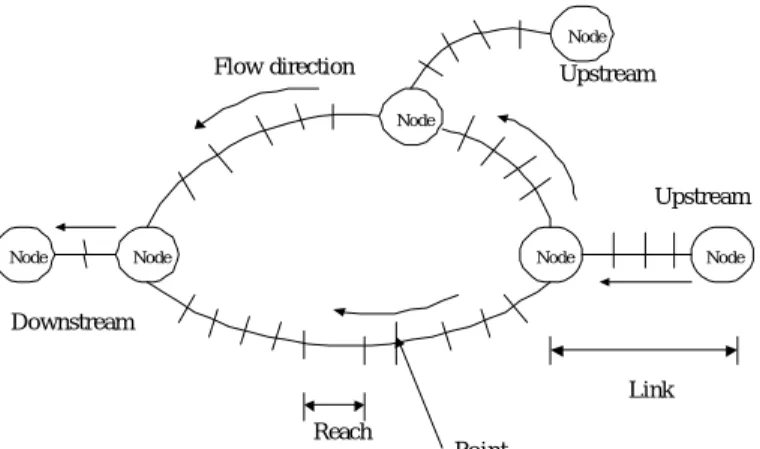
The definition sketch of the channel network is shown in Fig. 2, where the computational point represents the channel crosssection, the reach is the path between two computational points, the node is the junction of the river tributaries and the link represents the flow path between two nodes. The network
algorithm adopted in this model is similar to those of CHARIMA(Holly et al., 1990) with modification on hydraulic computation, sediment treatment, and some numerical schemes. The algorithm for hydraulic computation and sediment routing are discussed seperately as follows.
Node Node Node Node Node Upstream Downstream Flow direction Reach Point Link Node Upstream
Fig. 2 The definition sketch of the channel network 4.1 Hydraulic Routing
The flow discharge at the nodal point has to satisfy the continuity equation, i.e., the summation of the inflow and outflow discharges from all the tributaries at a nodal point must be zero, or there is no storage at the nodal point. The node continuity equation is:
Q Q m M m L j n j m n m 0, 1,2,..., ) ( 1 1 , 1+ = =
∑
= + +(16) where L m( ) = number of the links at node
m
, M = number of the nodes, j= identity of the links,Qm
n+1= discharge at node
m
during time n+1 and 1 , + nj m
Q = discharge from link j. Expressing
j m n j m n m Q Q Q , , 1= +∆ + , where n j m
Q, is a known value and ∆Qm,j is an unknown value to be solved, and the node continuity equation becomes
Q Q Q m M m L j j m m L j j m n m 0, 1,2,..., ) ( 1 , ) ( 1 , 1+
∑
+∑
∆ = = = = +(17) The nodal solution uses de St. Venant equations along the links between nodes to express the ∆Q
values in terms of corrections to water surface elevations at the nodes.
Concerning the linearized process and solutions which had been mentioned by Holly et al. (1990) , and will not be repeated herein. A relation among the water level changes at adjacent nodes is established by substituting some equations into the node continuity equation, equation (17). This leads to the matrix equation:
[
A
]{
∆
Y
}
=
{
B
}
(18) where [A]=a coefficient matrix comprising appropriate summations of some coefficients, {ΔY}=a matrix represents the water level changes and {B}=a known vector whose elements are imposed inflows, and sums of latest discharge estimates, some coefficients.
4.1.1 Solution strategy
The solution algorithm comprises three phases for each iteration: namely, link forward sweep, node matrix loading and link backward sweep. They are described as follows.
4.1.2 Link forward sweep
The detail process had been listed in the paper of Holly et al.(1990) for calculating coefficients at each computational point.
4.1.3 Node matrix loading
A. Upstream and downstream boundary conditions
In this model, the upstream boundary condition can be either stage or discharge hydrographs and there are three different ways to impose the downstream boundary conditions. They are discussed separately as follows:
a. Discharge hydrograph:
Impose the inflow and outflow discharge n+1
Q to the node continuity equation, i.e., equation (17), directly.
b. Stage hydrograph:
The downstream boundary condition can be replaced by:
n n Y Y Y= − ∆ +1
(19) c. Rating curve:
Using Taylor series expansion method to expand the stage-discharge relation, Q=f(y), and neglecting the higher order terms, the expression form becomes:
α∆Y+β∆Q=γ
(20) Comparing some equations, the water level variation ∆Y can be calculated. The corresponding downstream boundary condition can be obtained using the method proposed in previous section.
B. Node boundary conditions
Calculate the discharge, QI( j) and Q , at two ends of each link, and corresponding some coefficients. 1
Substitute these numbers into the matrix A and vector B shown in equation (18), and the water surface variations at the nodal point can be solved by the following equation.
{ } [ ] { } 1 B A Y = − ∆
(21) The block tri-diagonal matrix technique was adopted in this model to solve this equation.
4.1.4 Link backward sweep
Substitute the water surface variation ∆Y obtained at the nodal point into the derived ∆Q vs ∆Y
relation to calculate ∆Q1 and ∆QI( j). Then calculate ∆Y and ∆Q for each computational point,
from i=2 to i=I(j)-1, and then compute i n i n i Y Y Y +1+ +∆ and Q Qn Q i n i = +∆ +1 . 4.2 Sediment Routing
The bed elevation at a nodal point is assumed to be in an equilibrium condition, i.e., there is no net scouring and sediment deposition at the nodal point and total sediment flux at the nodal point equals to zero. Assuming the incoming sediment is fully mixed at the nodal point and then is distributed, according to the sediment transport capacity, to the downstream links. The bed load and suspended load are redistributed and treated separately at the nodal point. The definition sketch of the redistributions of the suspended load and bed load are shown in Fig. 3. They are discussed as follows.
4.2.1 Bed load transport
A bed load equation is used to calculate the bed load transport capacity at the first section downstream of the nodal point and a rating curve to describe the relationship between the flow discharge and the bed load transport capacity, Bc
b AcQ
Q = was established at the first section upstream of each link. Where
b
Q =the bed load transport capacity, and Ac and Bc=constants to be calibrated. The outflowing bed load transport rate is distributed according to the bed load transport capacity obtained from the rating curve. The nodal bed load continuity equation and the corresponding distribution principle at the nodal point only are listed as follows.
∑
(
)
∑
∑
∑
= = + + = = + + + = + ) ( 1 ) ( 1 1 , , 1 , ) ( 1 , , , , ) ( 1 1 , , 1 , , , m L j m L j n j m in n m b m L k B k out k c B j out j c m L j n j m b n m b out in out k c j c in in Q Q Q A Q A Q Q(22) where, Lin(m)=number of the links incoming toward the node m, Lout(m)=number of the links leaving the
node m and Lout,k=discharge leaving node m through link k.
Left bank Q 3 Q 1 Q 2 Q 4 Fully mixed Right bank Upstream Downtream Qs Qs Qs Qs C 2 C 3 C 4 Qs: Bed load C: Suspended concentration Q: Discharg e C 1
Fig. 3 The redistribution of suspended concentration and bed load at a nodal point
4.2.2 Suspended load transport
The suspended load is calculated by solving the sediment convection-dispersion equation using the split operator method. There are three portions, namely, Convection, longitudinal dispersion and reaction, involved in the split operator method and each portion has to be treated differently at the nodal point. The split operator method had been applied in numerical solution of the one- and two- dimensional convection-dispersion equation by Cunge, Holly, and Verwey, 1980. The algorithm used to split the sediment load at each node was originally proposed by Holly, Yang, et al. , 1990.
Convection:
The sediment concentration Ck and corresponding concentration gradient are assumed to be fully mixed
at the nodal point and then redistributed according to the weight of the flow discharge. The equations are expressed as:
, ,
∑
∑
= out in in k out k Q Q C C(23)
∑
∑
=
out in in k out kQ
Q
CX
CX
, ,(24) Longitudinal dispersion:
Assuming net flux of the suspended sediment due to the longitudinal dispersion effect equals to zero at a nodal point. The relation is expressed as:
∑
kxAtCXk=0(25)
Transverse dispersion and Reaction:
Since the suspended sediment is assumed fully-mixed at the nodal point and hence transverse dispersion and reaction treatments are not needed at the nodal point.
5 MODEL PERFORMANCE ASSESSMENT
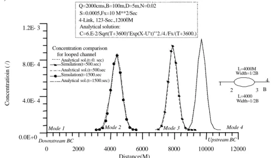
The numerical scheme for suspended load computation has been assessed by comparing it with an analytical solution and a set of experimental data (Lee and Yu, 1991). The results are shown in Fig. 4. It indicates that the algorithm performs well and the overall agreement is satisfactory. Please refer to Lee et al., (1997) for details of the assessments.
1 2 3 4 L=4000M Width=1/2B L=4000 Width=1/2B B 0 2000 4000 6000 8000 10000 12000 Distance(M) 0.0E+0 4.0E -4 8.0E-4 1.2E- 3 C oncentratioin ( /) Q=2000cms,B=100m,D=5m,N=0.02 S=0.0005,Fx=10 M**2/Sec ec 4-Link, 123-Sec.,12000M Analytical solution: -C=6.E-2/Sqrt(T+3600)*Exp(X-U*t)**2./4./Fx/(T+3600.)
Analytical sol.(t=0. sec) Simulation(t=500.sec) Analytical sol.(t=500.sec Simulation(t=1500.sec Analytical sol.(t=1500.sec)
Mode 1 Mode 2 Mode 3 Mode 4
Upstream BC Downstream BC
Concentration comparison
for looped channel
Fig. 4 Longitudinal variations of suspended concentration,
compared with analytical solution in a looped network
6 APPLICATION TO TANHSUI RIVER SYSTEM
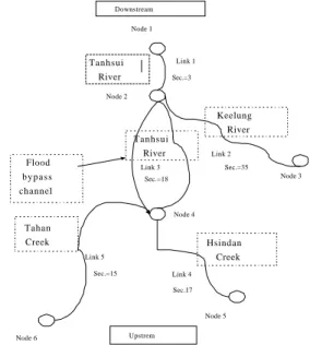
The Tanhusi River system passes through Taipei area, and is one of the most important river in Taiwan. It is a classified study case of tree-type channel network. It consists of of three branches, namely, Keelung River, Hsindan Creek , Tahan Creek, and one flood by pass channel, is a typical channel network. The location map is shown in Fig. 5.
This network consists of 5 links, 6 nodes and 88 crosssections and is within the estuarine area. The skematic diagram is shown in Fig. 6. There are five gage stations, namely, Hsiehchitou (link 1, Sec.3), Tachi bridge (link 2, Sec.20), Taipei bridge (link 3, Sec.13), Chongcheng bridge (link 4, Sec.10) and the entrance weir of the flood by pass channel (link 5, Sec.1), in the study area.
Tanhsui River Keelung River Hsindan Creek Tahan Creek Node 1 Node 2 Node 3 Node 4 Node 5 Node 6 Link 5 Sec.=15 Link 4 Sec.17 Link 3 Sec.=18 Link 2 Sec.=35 Link 1 Sec.=3 Tanhsui River Downstream Upstrem Flood bypass channel
Fig. 6 The skematic diagram of Tnahsui River network
These data, including water stages and channel bed variations, can be used to calibrate and verify the model. Field data from 1989, including geometric cross-sectional data and bed material data, are used as the inital condition. Data from 1989 to 1990 were used to calibrate the model and data from 1990 to 1991 were used for verification. Past experience and field observations indicate that there is insignificant sediment transport for flow discharge smaller than 100 m3/sec. Therefore, only discharges greater than
100 m3/sec are selected as the input flow conditions. The upstream inflow suspended sediment
concentrations versus the inflow water discharge rating curves obtained by the Taiwan Provincial Water Resources Department are used for the upstream boundary conditions. At the downstream boundary, which is located at Tudigonbi (Link 1, Sec.1), the measured stage hydrographs are used as the downstream boundary conditions. The model has to be "spinned" before real computation proceeds. A flow condition was assigned and let the model run until the water stages and discharges are smoothly-connected in the channel network, and this condition serves as the initial condition. The initial conditions for the sediment concentrations were then determined by the corresponding rating curves. The data of 1990 were used to calibrate the model. A time interval of 1 hour was used in the simulation and the total simulation period is 1489 hours. The Nt value of the thickness of the active layer is set to 1.0,
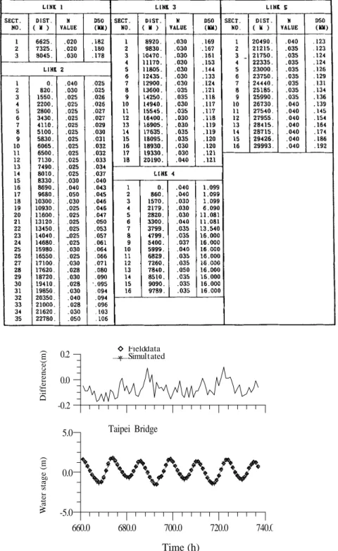
and the tube number chosen was 5. The ranges of size fraction are from 0.016 mm to 16.0 mm. The D50
values of bed material are shown in Table 1.
6.1 Parameter Examination
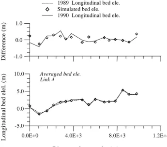
The measured water stage data from five different gage stations were used to calibrate the Manning's n value of the model. According to our experience, to independently increase the Manning’s value is especially needed on the estuary, bridge and bending situation in order to response real variance of water stage. The calibrated Manning's n values are also shown in the Table 1. The agreements are very good. The simulation results of Taipei bridge are shown in Fig. 7. The dispersion coefficients in both longitudinal and lateral directions have to be examined for the simulation of suspended load transport. However, due to the lack of sufficient field data, the relations from the author's previous study (Lee, et al., 1997) were adopted. The simulated bed elevations for links 1, 3, 5, and link 4 are shown in Figs. 8, and 9 respectively. The transverse bed profile of, link 4, Sec.10 is given in Fig. 10. The water stage result of real time shown in Fig. 7 is possessed of tidal characteristics, so it is suited to be simulated for using the
unsteady flow method. Fig. 8 and 9 show that the difference field of longitudinal bed elevation is clearly stated for the fitti ng result between measure and simulation. The match condition of bed evolution is good on some segment especially for link 4. The agreements are satisfactory.
Table 1 The Manning’s n value of the Tanhsui River System
-5.0 0.0 5.0
W
a
te
r
st
ag
e(
m
)
660.0 680.0 700.0 720.0 740.0Time (hrs)
FIELD DATA SIMULTATED -0.2 0.0 0.2 D if fe re n ce (m ) Taipei Bridge Fielddata Simultated Time (h) W ater stage (m) Difference(m)-10.0
-5.0
0.0 5.0 10.0
Longitudinal bed ele.(m) Difference(m) 5.0E+3 1.0E+4 1.5E+4 2.0E+4 2.5E+4 3.0E+4
Distance from outlet(m) 1989 Longitudina bed ele.
Simulated bed ele. 1990 Longitudinal bed ele.
-2.0 0.0 2.0
A v e r a g e d b e d e l e . L i n k 1 . 3 . 5 .
Fig. 8 The calibrated longitudinal bed elevations for links 1, 3 and 5
-5.0 0.0 5.0 10.0
Longitudinal bed elel. (m) Difference (m) 0.0E+0 4.0E+3 8.0E+3 1.2E+4
Distance from outlet (m)
1989 Longitudinal bed ele. Simulated bed ele. 1990 Longitudinal bed ele.
-1.0 0.0 1.0
Averaged bed ele. Link 4
Fig. 9 The calibrated longitudinal bed elevations for link 4
200 400 600
Cross-sectional distance (m) -5.0
5.0
Cross
-sec. bed ele.
1989 Cross-sec. bed ele. Simulated bed ele. 1990 Cross-sec. bed ele.
6.2 Verification
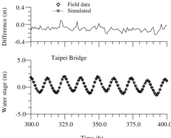
Using the parameters determined in the previous analysis, the model is applied to simulate the channel bed evolutions of Tanhsui River System from 1990 to 1991. The total simulation period is 672 hours. The comparisons of the longitudinal water surface elevations, longitudinal bed profiles and cross-sectional bed profiles are shown in Figs. 11, 12, 13, and 14 respectively. Fig.11 shows that using the calibrated Manning's n value, the model can simulate the temporal variations of the water surface elevations very accurately. The simulated longitudinal and transverse bed profiles are shown in Figs. 12, 13, and 14, respectively. In the verification process, it seems to be fine rather link 1,3,5 than link 4 for the simulated results of bed evolution. The overall accuracy is good.
-5.0 0.0 5.0
Water stage (m) Difference (m)
300.0 325.0 350.0 375.0 400.0 Time (h) Field data Simulated -0.4 0.0 0.4 Taipei Bridge
Fig. 11 The verified water surface elevations at the Taipei Bridge
-10.0 -5.0 0.0 5.0 10.0
Longitudinal bed ele. (m) Difference (m) 5.0E+3 1.0E+4 1.5E+4 2.0E+4 2.5E+4 3.0E+4
Distance from Outlet (m) 1990 Longitudinal bed ele. Simulated bed ele. 1991 Longitudinal bed ele.
-2.0 0.0 2.0
Aberaged bed ele. Link 1.3.5.
-10.0 -5.0 0.0 5.0 10.0
Longitudinal bed ele. (m) Difference (m) 5.0E+3 1.0E+4 1.5E+4 2.0E+4 2.5E+4 3.0E+4
Distance from outlet (m) 1990 Longitudinal bed ele. Simulated bed ele. 1991 Longitudinal bed ele.
-2.0 0.0 2.0
Aberaged bed ele. Link 1.3.5.
Fig. 13 The verified longitudinal bed elevations for link 4
200 300 400 500 600
Cross-sectional distance (m)
-5.0
5.0
Cross
-sec. bed ele. (m)
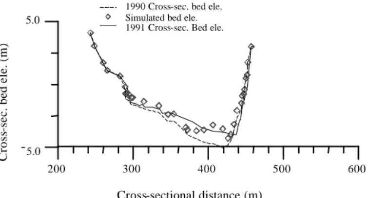
1990 Cross-sec. bed ele. Simulated bed ele. 1991 Cross-sec. Bed ele.
Fig. 14 The verified transverse bed profiles for links 4, sec.10
7 APPLICATION TO CHICHI HYDRAULIC MODEL STUDY
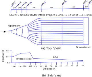
The Chichi common water intake project, which is currently under construction, is located in central Taiwan. One of the key facilities in this project is the sediment desilting basin. It is a looped-type case to be shown herein. It consists of 12 subchannels and is able to perform sediment flushing and water inta king simutaneously. A series of hydraulic model studies were conducted by Taiwan Provincial Water Resources Department to investigate the sediment flushing efficienc y of this layout, and these studies provide a very good data set to verify the sediment allocation algorithm of the NETSTARS. The layout of this sedimentation basin is shown in Fig. 15.
It consists of 14 links, 4 nodes and 199 crosssections. The particles used in the model studies ranges from 0.125 mm to 4.0 mm and the mean particle size is 1.0 mm. The distance between Sec.1 and Sec.4 is about 40 m and an adverse slope, with a slope of 1/50, is constructed to generate a steady flow condition near the inl et. The elevation varies from 0 to 2.5 m and then drops to -1.2 m, the design
inflow discharge was selected to be 44.5 cms and three different inflow concentrations, which equals 5000, 3000 and 1000 ppm, respectively, were tested in the experiments. The corresponding experimental durations equal to 10, 16 and 36 hours, respectively. The deposition process had been found on the adverse slope in this experiment, but the deposited height and distribution not been measured by experimenters. That is to say, only the deposition behavior in subchannels is observed and recorded. The average value of deposition in subchannels is recorded, so the stream tube number chosen is 1 for simulation in order to reflect the average bed evolution on each section. The time interval Δt is set to be 10 min and the measured water surface variations were used as the downstream boundary conditions. The initial conditions were obtained from the same spinning process as the Tanhsui River study. The simulated bed profiles of channel F for three different sediment concentrations are shown in Figs. 16, 17 and 18, respectively. The deposition condition is not consistent in the upstream segment for different inflow concentration. The drop phenomenon of water stage happens due to depositi on being formed or sediment inflow being increased on inlet in the case of the inflow concentration equaling to 3000 and 5000 ppm. The control flow condition is produced on the sec.3, and it shows that the supercritical flow condition happens herein in the simulated process, too. The overall agreement is acceptable.
se c-1 se c-2 se c-3 se c-4 se c-5 se c-6 se c-7 se c-8 10M 10M 10M 25M 40M 40M 10M 140 130 120 110 100 90 80 70 60 50 40 30 20 10 4. 0 0. 0 -4. 0 E le v a ti o n (M ) In v e rs e s lo p e 1/50 Dis tan c e (M ) D ow ns tre am U ps tre am
C hic h i C om m o n W a te r Intak e Pro jec t(1 Lin k -- -> 12 Lin k s - -- > 1 lin ks )
(a) Top View
(b) S ide V ie w
Fig. 15 Layout of the sediment desilting basin of Chichi Common Water Intake Project
0.0 40.0
80.0 120.0
160.0
Distance from outlet (m)
-5.0 0.0 5.0 10.0 15.0 Bed thalweg (m)
Comparison thalweg(Duration=10hrs) Q=44.5 CMS , C=5000PPM
Initial bed thalweg Measured bed thalweg Computed bed thalweg Chichi common water intake project
Computed water stage
0.0 40.0
80.0 120.0
160.0
Distance from outlet (m)
-5.0 0.0 5.0 10.0 15.0 Bed thalweg (m)
Comparison thalweg (Duration=16 hrs) Q=44.5 CMS , C=3000 PPM
Initial bed thalweg Measured bed thalweg Computed bed thalweg
Chichi common water intake project
Computed stage water
Fig. 17 The calibrated channel bed variations of subchannel F(C=3000 ppm)
0.0 40.0
80.0 120.0
160.0
Distance fromoutlet (m) -5.0 0.0 5.0 10.0 15.0 Bed thalweg (m)
Comparison thalweg (Duration=36 hrs) Q=44.5 CMS ,C=1000 PPM
Initial bed thalweg Measured bed thalweg Computed bed thalweg Chichi common waterintake project
Computed water stage
Fig. 18 The verified channel bed variations of subchannel F(C=1000 ppm) 8 CONCLUSIONS
A numerical model, which is capable of simulating scouring and deposition behaviors in a channel network under an unsteady flow condition, is developed in this study. A state-of-the-art sediment routing algorithm which is capable of simulating suspended and bed loads seperately was develo ped in this model. An internal boundary condition based on the sediment transport capacity was proposed to distribute the incoming sediment load into the dow nstream links. The proposed measure is proved to be feasible.
The model's performance and applica bility have been demonstrated through an application to the Tanhsui River system and the hydraulic model studies of the sediment desilting basin of the Chichi water supply project. Convincing results are obtained.
ACKNOWLEDGEMENT
This study is financially supported by the Sinotech Research Foundation. Helpful comments from Mr. Hsu, R.L., Mr. Chen, L.M. and Mr. Hsieh, K.C., of the Sinotech Consultant Company and Dr. Yang, C.T. from U.S. Bureau of Reclamation are appreciated.
REFERENCE
Bennet, J.P. and Nordin, C.F. 1977, Simulation of sediment transport and armouring. Hydrological Sciences Bulletin, XXII.
Chang, H. H. & Hill, J. C. 1976, Computer modelling of erodible flood channels and deltas, Journal of the Hydraulics Division, ASCE, Vol. 102, No. HY10, pp. 132-140.
Cunge,J.A., Holly,F.M.,Jr, and Verwey, A. 1980, Practical Aspects of Computational River Hydraulics, Pitman Publishing Ltd., London, 00, pp. 312-349.
Elder,J.W. 1959, The dispersion of marked fluid in turbulent shear flow. Journal of Fluid Mechanics, 5, No. 4, pp. 544-560.
Holly, F.M., and Preissmann, A. 1977, Accurate calculation of transport in two dimensions. Journal of Hydraulic Division, ASCE, Vol. 103, No. HY11, pp. 1259-1277.
Holly, F.M. ,and Rahuel, J.L. 1990, New numerical/physical framework for mobile-bed modeling. Part I, Journal of Hydraulic Research, Vol. 28, No. 4.
Holly, F.M., Yang, J.C., Schovarz, P., Scheefer J., Hsu, S.H. and Einhellig, R. 1990, CHARIMA numerical simulation of unsteady water and sediment movements in multiply connected networks of mobile -bed channels. IIHR Report No. 0343, The University of Iowa, Iowa City, Iowa, U.S.A.
Holly, F.M., Yang, J.C. and Spasojevic, M. 1985, Numerical simulation of water and sediment movement in multi-connected networks of mobile bed. Iowa Institute of Hydraulic Research, Limited Distribution Report No. 131, The University of Iowa, Iowa City, Iowa, U.S.A.
Karim, M.F. and Kenndy, J.F. 1982, IALLUVIAL: A Computer-based flow and sediment routing for alluvial streams and its application to the Missouri River, Iowa Institute of Hydraulic Research, Report No. 250, The Un iversity of Iowa, Iowa, USA.
Lai, C. T. 1986, Numerical modeling of unsteady open-channel flow. Advances in Hydroscience, Vol. 14. U.S. Geological Survey National Center Reston, Virginia, pp. 225.
Lee, H.Y., and Yu, W.S. 1991, An experimental study on reservoir sedimentation. Hydraulic Research Laboratory Report, National Taiwan University, Taiwan, (in Chinese).
Lee, H.Y., Hsieh, H.M., Yang, J.C. and Yang, C.T. 1997, Quasi-two-dimensional simulation of scour and deposition in alluvial channels. Journal of Hydraulic Engineering, ASCE, Vol. 123, No. 7, July, pp. 600-609.
Lin, B. 1984, Current study of unsteady transport of sediment in China. Processings of Japan-China Bi-Lateral Seminar on River Hydraulics and Engineering Experiences, July, Tokyo-Kyoto-Sapporo, pp. 337-342.
Lyn,D.A., and Goodwin,P. 1987, Stability of a general preissmann scheme. Journal of Hydraulic Engineering, ASCE, Vol. 103, No. HY1, pp.16-27.
Meyer-Peter,E. and Mueller,R. 1948, Formulas for bed-load transport, International Association for Hydraulic Research , 2nd Meeting, Stockholm.
Molinas, A.M. and Yang, C.T. 1986, Computer Program User's Manual for GSTARS, U.S. Department of Interior Bureau of Reclamation, Engineering and Research Center, Denver, Colorado.
Simons & Li Assoc. Inc. 1980, Scour and Sediment Analysis of the Proposed Channel of the Salt River for Protection of the Sky Harbor International Airport in Phoenix, Arizona, Howards, Needles, Tammon and Bergondoff, Kansas City, Missouri, USA.
Spasojevic, M. and Holly, F.M. 1988, Numerical simulation of two -dimensional depostion and erosion patterns in alluvial water bodies. IIHR Report No. 149, the University of Iowa, Iowa City, Iowa, U.S.A.
Thomas, W. A. and Mcanally, W. H., Jr. 1985, User's Manual for the Generalized Computer Program System Open Channel Flow and Sedimentation TABS-2, Department of the Army Waterways Experiment Station, Corps of Engineers, Vicksburg, Mississippi, USA.
Thomas, W. A. & Prashum, A. L., 1977, Mathematical model of scour and deposition. Journal of the Hydraulics Division, ASCE, Vol. 110, No. HY11, pp. 1613-1641.
LIST OF SYMBOLS
A channel cross-sectional area;
Adt amount of sediment scouring/deposition per unit length of the channel;
at reference level above bed;
Bt width of the channel;
Cdk deposition concentration in terms of solids volume per unit fluid volume;
Cek sediment concentration close to the channel bed;
Ck depth-averaged concentration of the suspended sediment of size fraction k;
c'
Chezy coefficient related to grains =
90 3 12 log 18 D Rt ; Dk particle diameter of size fraction k;
Dó particle parameter = 3 / 1 2 50 ) 1 ( − v g s D ; G gravitational acceleration; h flow depth;
j identity of the links; K channel conveyance;
kx longitudinal dispersion coefficients;
kz transverse dispersion coefficients;
Lin(m) number of the links incoming toward the node m;
Lout(m) number of the links leaving the node m;
n roughness coefficient of Manning's formula; M number of the nodes;
Pi wetted parameter;
p channel bed porosity; Q flow discharge; Qb bed load transport rate;
Qout,k discharge leaving node m through link k;
1 , + n j m
Q discharge from link j;
1 + n m
Q discharge at node m during time n+1;
q lateral inflow/outflow discharge per unit length;
qb bed load discharge in solids weight per unit time, and per unit width;
R hydraulic radius;
Sdk the amount of sediment deposition;
Sek the amount of sediment resuspension;
Sf energy slope;
Sk source term of the suspended sediment of size fraction k;
s specific weight of sediment particle; Tk
transport stage parameter = 2
* 2 * 2 ' * ) ( ) ( ) ( cr cr u u u − ; t Time; U average velocity; uó shear velocity; uócr critical shear velocity;
*
u
′
grain shear velocity =' 5 . 0 c u g ; W fall velocity of sediment particle; Wk fall velocity of sediment of size fraction k;
x coordinate in the flow direction; y water surface elevation;
z coordinate in the transverse direction;
α momentum correction coefficient;
βk weight percentage of sediment of size fraction k;
κ Karman's constant;
ν water kinematic viscosity;
ρs sediment density;
ΔQ the increments of discharge surface elevation for every point during iteration; ΔY the increments of water surface elevation for every point during iteration; ΔZi variation of the bed elevation for every size fraction.