大型工作的即時排程演算法之研究

行政院國家科學委員會專題研究計畫 成果報告

大型工作的即時排程演算法之研究

計畫類別： 個別型計畫

計畫編號： NSC93-2213-E-011-074-

執行期間： 93 年 08 月 01 日至 94 年 07 月 31 日 執行單位： 國立臺灣科技大學資訊管理系

計畫主持人： 徐俊傑

報告類型： 精簡報告

處理方式： 本計畫涉及專利或其他智慧財產權，1 年後可公開查詢

中 華 民 國 94 年 8 月 31 日

行政院國家科學委員會補助專題研究計畫 ■ 成 果 報 告

□期中進度報告

大型工作的即時排程演算法之研究

計畫類別：■ 個別型計畫 □ 整合型計畫 計畫編號：NSC93-2213-E-011-074

執行期間： 93 年 08 月 01 日至 94 年 07 月 31 日

計畫主持人： 徐俊傑 共同主持人：

計畫參與人員：

成果報告類型(依經費核定清單規定繳交)：□精簡報告 □完整報告

本成果報告包括以下應繳交之附件：

□赴國外出差或研習心得報告一份

□赴大陸地區出差或研習心得報告一份

□出席國際學術會議心得報告及發表之論文各一份

□國際合作研究計畫國外研究報告書一份

處理方式：除產學合作研究計畫、提升產業技術及人才培育研究計畫、

列管計畫及下列情形者外，得立即公開查詢

□涉及專利或其他智慧財產權，□一年□二年後可公開查詢 執行單位：國立臺灣科技大學資管系

中 華 民 國 九十四 年 七 月 三十一 日

附件一

行政院國家科學委員會專題研究計畫成果報告 大型工作的即時排程演算法之研究

計畫編號：NSC93-2213-E-011-074 執行期限：93 年 08 月 01 日至 94 年 07 月 31 日

主持人：徐俊傑 國立臺灣科技大學資管系

一、中文摘要

大型工作(Supertask)首次由 Moir 與 Ramamthy 兩 人所提出，並且應用在比例式公平(Proportionate fairness, Pfair)的排程中。當某些工作被限定在同 一個處理器上面執行時，可將這些工作組合起來 成為一個大型工作，並且被視為一般的 Pfair 工 作來進行排程。也就是說, 當它(大型工作)被排 程時, 它所包含的其中一個工作（又稱為子工作 (component task)）就會被挑出來執行。然而，這 些 工 作 並 不 能 保 証 可 以 在 他 們 各 自 的 期 限 (deadlines)內完成。因此，大型工作的概念還無 法應用在對時間有嚴格要求的即時系統之中。

Holman 與 Anderson 就提出了一種重新加權的演 算法來改善 Moir 等人所提出的方法。這種方式 是藉由增加大型工作的執行權重(task weight)，而 增加對系統需求的頻率，進而滿足其內部子工作 的執行需求。他們的方法保證每一個子工作都能 夠在他們各自的期限內完成。然而，根據他們的 實驗結果，這種重新加權的演算法會大幅增加系 統閒置的時間。在這篇論文中，其目標是要降低 系統閒置時間。也就是說，儘可能降低大型工作 的重新加權的幅度(inflation)與次數。首先，我們 提出大型工作的瞬時行為預測(Transient Behavior Prediction，TBP)的概念。TBP 是用來預測每一個 Pfair 工作請求“最晚”以及“最早”會被安排 在相對應的 Pfair window 中第幾個時槽。根據這 種概念，我們提出一個在時間上更有效率的可排 程性(schedulability)演算法。它可以有效率地找出 哪些大型工作可以不經重新加權即可保證其內 部的子工作都能在期限內完成。另外，針對那些 有可能會使其子工作超出期限的大型工作，我們 提出工作合併的演算法，使這些大型工作能在不 必重新加權的情況下，利用與其它工作合併的方 式增加其權重並避免其子工作超出期限。最後，

針對這些剩餘無法合併的大型工作，我們提出一 個更有效率的重新加權公式。它能夠大幅降低大 型工作加權後的膨脹係數(加權後的權重減去加 權前的權重)。根據實驗結果，可以發現這本計

劃所提出的方法在執行時間上更短，並且大幅降 低工作平均膨脹係數與重新加權的次數。

關鍵詞：大型工作，即時系統排程，比例式公平排程，最

早虛擬期限優先。

Abstract

The supertask approach was proposed by Moir and Ramamthy as a means of supporting non-migratory tasks in Pfair-scheduled systems. In this approach, tasks bound to the same processor are combined into a single server task, called a

supertask, which is scheduled as an ordinary Pfair

task. When a supertask is scheduled, one of its component tasks is selected for execution. In previous work, Holman et al. showed that component-task deadlines can be guaranteed by inflating each supertask’sutilization.In addition, their experimental results showed that the required inflation factors should be small in practice.

Consequently, the average inflation produced by their rules is much greater than that actually required by the supertasks.

In this project, we first propose a notion of

Transient Behavior Prediction for supertasks,

which predicts the latest possible finish time of subtasks that belong to supertasks. On the basis of the notion, we present an efficient schedulability algorithm for Pfair supertasks in which the deadlines of all component tasks can be guaranteed. In addition, we propose a task merging process which combines the unschedulable supertasks with some Pfair tasks;

hence, a newly supertask can be scheduled in the system. Finally, we propose the new reweighting functions that can be used when the previous two methods fail. Our reweighting functions produce smaller inflation factor than the previous work does. To demonstrate the efficacy of the supertasking approach, we present the experimental evaluations of our algorithm, which decreases substantially a number of reweights and the size of inflation when there are many

supertasks in the Pfair-scheduled systems.

keywords: supertasks, real-time scheduling, Pfair,

EPDF.

二、緣由與目的

Proportionate-fair (Pfair) scheduling, proposed by Baruah et al.[1,2,3,4,7,8,9,12,24], is presently the only known optimal scheme for scheduling recurrent real-time tasks on a multiprocessor system. The Pfair scheduling algorithms presented in [8,9] are based on the assumption that tasks(or parts thereof) can be executed on any processor and that tasks can be suspended on one processor and resumed on another at any time; in other words, tasks must be able to migrate between processors if necessary.

However, a task model in which all tasks are able to migrate may be unrealistic[24], because some tasks may need to run a particular processor. Suppose, for example, that we wish to schedule tasks on the processors of a set of workstations in a LAN. If some tasks read data from a device that is physically located in or connected to one of the machines, then that tasks must execute in their entirety in that particular machine and cannot be migrated to another processor.

Moir and Ramamurthy [24] proposed the supertask approach [18,19,20]. In this approach, the non-migratory tasks bound to a specific processor are combined to be a s i ngl e “ s upe r t a s k, ” whi c h i s t hen s c he dul e d a s a n or di na r y Pfair task; when a supertask is scheduled, one of its component tasks is selected for execution. Unfortunately, although Mo i r a nd Ra ma mur t hy’ s pape r s ugge s t s t ha t supertasking is a promising approach, counterexamples presented by them show that non-migratory tasks may miss their deadlines when supertasking is used in conjunction with priority definitions PF[8], PD[9], or PD

²

[1,2].

Nevertheless, Holman et al.[18] proved that such violations can be avoided by using a pessimistic weight assignment. In other words, they proposed reweighting rules (EPDF-Liner and EPDF-Exponential) to inflate the s upe r t a s k’ s we i ght , thus preventing the component-task misallocations in a supertask. Unfortunately, these reweighting rules will always result in a lot of schedulability loss. Besides, a large portion of supertasks in a multi-supertask system, indeed, needs not to be reweighted, nor can their rules distinguish the supertasks which need not to be reweighted.

Example. To see the drawback of the reweighting

algorithms in literature, consider the two-processor Pfair schedule shown in Figure 1.1(a). In the Pfair literature, the ratio of tasks’ exe c ut i on c os t t o i t s pe r i od i s r e f e r r e d t o a s i t s we i ght ; a t a s k’ s we i ght de t e r mi ne s t he l e ngt h a nd the alignment of its Pfair windows. The task set in Figure 1.1(a) consists of four normal tasks T

₁

, T

₂

, T

₃

and T

₄

with weight

11 6 9 2 9 2 50

11

, , and , respectively, along with three supertasks, T

₂

, T

₃

and T

₄

, which represent two component tasks CT

₁

-CT

₂

with weight

72 7 8

1

, , two component tasks CT

3

-CT

4

with weight

45 1 5

1

, and two component tasks CT

₅

-CT

₆

with weight

55 3 55

27

, , respectively (shown in the lower region). T

₂

competes with a weight of

9 2 72

7 8

1

  , T

₃

competes with a

weight of

9 2 45

1 5

1

  and T

₄

competes with a weight of

11 6 55

3 55

27

  . In the figure, each subtask window is indicated by a mark interval; for instance, the first window of T

₁

spans the interval  

0,5

. An “ ▄”is used to denote the quantum allocated to a subtask; for example, the first subtask of T

1

is scheduled in time slot 0. All scheduling decisions in the upper region are compatible with the PD

²

Pfair algorithm. In the lower region, allocations within T

₂

, T

₃

and T

₄

are shown.

These allocations are based on the earliest pseudo-deadline-first (EPDF) priorities. Under EPDF scheduling, an Earliest- Pseudo-Deadline rule is used to prioritize subtasks, with tie broken arbitrarily.

11/50 T1

2/9 T2

2/9 T3

6/11 T4

Missed Deadline 1/8

CT1

7/72 CT2

1/5 CT3

1/45 CT4

27/55 CT5

3/55 CT6

Within T2

Within T3

Within T4

11/50 T1

2/5 T2

2/5 T3

1/1 T4

1/8 CT1

7/72 CT2

1/5 CT3

1/45 CT4

27/55 CT5

3/55 CT6

Within T2

Within T3

Within T4

Fig. 1.1: PD²/EPDF schedule with a (a) regular and (b) reweighted supertasks T2, T3and T4on two processors.

Figure 1.1(a).

As the schedule showed in Figure 1.1(a), CT

₃

misses a pseudo-deadline at time slot 9 because no quantum is allocated to T

₃

in the interval  ^{5 , 10}  , which contains one component task window and no undivided supertask windows. In Figure 1.1(b), the reweighting rules [18]

proposed by Holman et al.

produce significant schedulability loss; after inflating T

_2,

T

₃

and T

₄

, the rules waste almost half of their utilization (three and eight scheduled slots, respectively). Hence, the instance in Figure 1.1 (b) needs three processors(

1 2

5 2 5 2 50

11

 

 

). However, see Figure 1.1(c), T

₂

could satisfy the quantum demand of CT

₁

and CT

₂

without any inflation, T

₃

can be reweighted by slighter inflation. Also, T’

₄

is composed of T

₁

and T

₄

in Figure 1.1(a) so that its component tasks can be ensured to meet their deadlines. Unfortunately, this situation will go from bad to worse when the proportion of supertasks to all tasks of the system increases. The example and the experimental results as stated by Holman et al. also show that the required inflation factors should be very small in practice, especially in multi-Pfair-supertask systems.

In this paper, we present reweighting functions where component tasks are EPDF-scheduled and the time values are integral. We propose a new algorithm and reweighting functions, which produce a smaller number of task reweights and smaller inflation. First, we propose a notion of Transient

2/9 T2

1/4 T3

421/550 T 4

1/8 CT1

7/72 CT2

1/5 CT3

1/45 CT4

27/55 CT5

3/55 CT7

Within T2

Within T3

Within T4

11/55 CT6

Figure 1.1(c). PD²/EPDF schedule with an improved algorithm to reduce (or eliminate) the inflation factor of supertask

T , T and T on two processors.

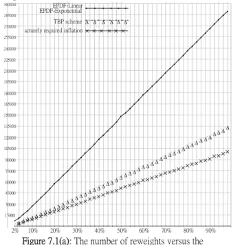
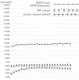
Behavior Prediction for supertasks. TBP predicts the latest possible finish time of subtasks associated with the supertasks. On the basis of the notion, we present an efficient schedulability algorithm for every supertask. This algorithm pr obe s whe t he r a l l c ompone nt t a s ks ’ de a dl i ne s can be guaranteed. If they are not, the algorithm would collect these supertasks and combine them separately with some original Pfair tasks to satisfy the schedulable conditions we proposed. Finally, if the above-mentioned schemes do not work on some supertasks, then we inflate them by using our reweighting functions that produce a smaller inflation factor than the previous work does. To demonstrate the efficacy of the supertasking approach, we present the experimental evaluations of our algorithm, which decreases substantially the frequency of reweight and the amount of inflation when there are many supertasks in the Pfair-scheduled systems.

The remainder of this paper is organized as follows. Sec.2 summarizes the background information and the notational conventions. In Sec.3, some properties of Pfair schedule are presented. In Sec.4, the schedulability conditions for supertasks and their component tasks are derived. Our reweighting functions and algorithm are then presented in Sec.5 and Sec.6, respectively. Sec.7 includes experimental results, which reveals the efficacy of using the proposed reweighting algorithm to substantially reduce schedulability loss. Finally, we conclude in Sec. 8.

二. Task Models

In this section, we introduce some concepts proposed in [3,18,27]. To present the notations about Pfair scheduling, we focus our attention on synchronous, periodic task systems. A periodic task T

_i

with an integer execution requirement T

_i

.e and an integer period T

_i

.p has weight wt(T

_i

)=T

_i

.e/T

_i

.p, where 0<wt(T

_i

)<1. A task T

_i

is heavy if wt(T

_i

)≧

2

1

, and light otherwise. In Pfair scheduled systems, scheduling decisions occur at integral values of time, numbered from 0. Moreover, the processor time is allocated in discrete time units, called quanta. The actual interval between time t and time t+1(including t, excluding t+1) will be referred to as time slot t, t. Besides, for integer a and b, b>a, let  a, b



={a,…,b-1}.The sequence of allocation decisions over time defines a schedule S which is a function from τ×Ν to {0, 1}, whereτis the set of n tasks to be scheduled and N is the set of nonnegative integers.

Informally, S(T

_i

,t)=1 if and only if task T

_i

is scheduled in time slot t. Certainly, in any M-processor schedule,



_ 

Ti S(Ti,t) M

holds for all t and









_ Ti wtTi

U U

M , ( )

denotes

the total amount of task weights. Let nonnegative integers n, m and M denote the quantity of tasks in setτ, supertasks and identical processors in systems, respectively.

2.1 Lags constraints.

The lag of a task T

_i

at time t with respect to schedule S, denoted as Lag(S, T

_i

, t) which is defined by:

Lag(S, T

_i

, t)= Share(T

_i

, t)－

 )[0,

( , )

t

j STi j

(1)

Where Share(T

_i

, t) =wt(T

_i

) × t . A schedule S is Pfair if and only if

T

_i

, t:: －1 < Lag(S, T

_i

, t) < 1. (2) As shown in (2), each task T

_i

can be divided into an infinite sequence of quantum-length subtasks. The j

^th

subtask(j≧1) of task T

_i

is denoted as T

_i,j

. As in [6] each subtask T

_i,j

has a pseudo-release r(T

_i,j

) and Pseudo-deadline d(T

_i,j

), as described below:

r(T

_i,j

)= 

^{j T}_Ti_e^p



i . ) . 1

( 

, d(T

_i,j

)=

. . . 

 



 e T

p jT

i

i

(3)

T

_i

must be scheduled in the interval

w

(

Ti,j

) 

r

(

Ti,j

),

d

(

Ti,j

) 

termed Pfair window, or Pfair will be broken. The length of T

_i,j

’ s Pfair window, denoted by |w(T

_i,j

)|, is d(T

_i,j

)－r(T

_i,j

).

Note that r(T

_i,j+1

) is either d(T

_i,j

)-1 or d(T

_i,j

), and the length of each task T

_i

’ s window is either

^_^T_Ti^i._.e^p_^

or

^_^T_Tⁱ_i^._.e^p_^

+1. We define the length of minimal and maximal window as

 

( ) 1

Ti

wt

and  

( )

¹

1



Ti wt

, respectively. The Task windows, the length of which is identical, are called uniform-length tasks. Besides, the Pfair schedules can be defined informally by subtracting an ideal fluid [21] in which wt(T

_i

) processor time is allocated to each task T

_i

in each slot. Besides, let T

_i

.mcw denote the shortest window of any component task of T

_i

and T

_i

.msw denote the shortest supertask window.

2.2 Supertasks

Let ST denote this supertask and let each component task CT have an execution requirement CT

_i

.e and a periodic CT

_i

.p.

The ratio CT

_i

.e/CT

_i

.p is called the weight of CT

_i

and is denoted as wt(CT

_i

). As in [18], since the supertasks are scheduled using reweighted criterion, ST’ s original parameters(before inflating) are ST.e, ST.p and weight wt(ST)=ST.e/ST.p, and its reweighted parameter resulting from inflation includes an execution requirement

ST ˆ

.

e

, period

_{ST ˆ}

_.

_p

as well as weight

_ST

.

_w

ˆ 

_ST

.

_e

ˆ /

_ST

.

_p

ˆ . For example, in Figure 1.1(a), T

₂

has original parameters T

₂

.e=2, T

₂

.p=9 and wt(T

₂

)=2/9. Its reweighted parameters are T ˆ

²

. e =1,

p

T ˆ

²

. =4 and T

2

. w ˆ =1/4 in Figure 1.1(c). For consistency, we also use this notation for component tasks understanding that

e

Ti

. , _T

i

. _p and

_Ti

.

_w

are equivalent to T

ⁱ

. , e ˆ T

i

. p ˆ and T

i

. w ˆ , respectively. Consequently, we define the actual weight of a supertask ST as wt(ST)= 

CTST i

i wt

(

CT

) , and ST’ s inflation factor is derived by subtracting wt(ST) from ST ˆ . . w

2.3 Transient Behavior Prediction.

As to the prior knowledge of Pfair schedule, one quantum necessitates to be allocated to every Pfair window.

Seemingly, the places of quanta with respect to their windows are scattered across their Pfair windows. However, this transient behavior is regulated by numerous system parameters. Basically, this behavior is directed by task weights, processor number and priority definitions such as EDF, EPDF etc. In order to predict the locations of the scheduled quanta with respect to their Pfair-window, we start off by defining these notations below.

) , ( T

,

S

F

i j

denotes the distance from r(T

_i,j

) to the finish time of subtask T

_i,j

in schedule S.

) ( T

i

LPF denotes the latest possible finish time that a

task inherits during its execution time, that is, the longest F ( T

i,j

, S ) in T

i

.

) ( T

i

MD denotes the maximum distance between two consecutive quanta allocated to each T

_i

.

An example of the above notations is shown in Figure 2.1.

Figure 2.1 : The exam ple of Pfair tasks illustrates the

notations

F(Tⁱ,^j

),

LPF(Tⁱ

) and

M D (Tⁱ

).

M D(T0)=6 L PF(T0)=4

F(T0,1)=2 F(T0,2)=4 F(T0,3)=4 F(T0,4)=2

) (Ti

LPF

and

MD

₍

Ti

₎ denote the estimations of )

( T

ⁱ

LPF and MD ₍ T

i

₎ , respectively.

Roughly, the part of our works aims at approaching LPF ( T

i

) by

LPF

₍

Ti

₎ and at taking advantage of it to calculate

_MD

₍

_Ti

₎ . The accuracy of

_MD

₍

_Ti

₎ in this paper plays a crucial role determining directly the efficacy of our reweighting functions and the schedulability test procedure.

3. Some properties of

LPF ( T

ⁱ

)

and

MD ( T

ⁱ

) The following lemma introduces a simple notion that characterizes the diverse lengths of task windows. Lemma 3.1 and Lemma 3.2 follow directly from the proof of properties (P1) through (P8) in [2].

Lemma 3.1. (diversity window-lengths lemma)

For all tasks weight wt(T

_i

)=T

_i

.e/T

_i

.p, T

_i

.e and T

_i

.p are relative primes. T

_i

.p mod T

_i

.e ≦ 1 if and only if task T

_i

has identical length Pfair windows.

According to Lemma 3.1 and the results shown in [2], the conditions of uniform-length windows can be rewritten as follows:

Ti.p mod Ti.e≦1, Ti

’ s Pfair windows have identical length of  

Te p T

i i . .

.

Ti.p mod Ti.e≧2, Ti

’ s Pfair windows have lengths of either  

_T^Ti_e^p i

.

. or

 

^T_T^.i_.e^{p 1}

i

.

As mentioned in Figure 1.1(a), because task T

₂

has T

₂

.p mod T

₂

.e=1, it has identical window length of five. Similarly, since T

₁

has T

₁

.p mod T

₁

.e=6, it has two kinds of window lengths. For example, T

_1,1

and T

_1,2

have lengths of five and six, respectively. By Lemma 3.1, the connections between

) (

Ti

MD

and LPF ₍ T

i

₎ can be expressed as

In Figure3.1(a), if all continuous windows are minimal windows and

LPF₍Ti₎

is given, then the maximum distance between these two consecutive quanta is  

. ^{( ) 2}

.  i 

e T

p

T LPF T

i

i

.

Likewise, if there exist maximal windows in that task (see Figure 3.1 (b)), the maximum distance for every pair of consecutive quanta is not longer than

 . ^{( ) 1.}

.  i

e T

p

T LPFT

i i

window(Ti,k)









i i

c p window(Ti,k-1)

1 ) (

1 





 





i i

i LPF T

c p









i i

c p

Figure 3.1(a):Ti.p mod Ti.e^1

1 ) ( . 1

. 

 



 i

i

i LPFT

e T

p T



 



 e T

p T

i i .

. 

 



 e T

p T

i i . .

Lemma 3.2. (the sum

of overlaps within an interval)

Let wt(T

_i

)=T

_i

.e/T

_i

.p and 1>wt(T

_i

)>0. If T

_i

.e and T

_i

.p are relative primes, and T

_i

.e>1, then there exists T

_i

.e-1 overlaps in interval l=[k × T

_i

.p, (k+1) × T

_i

.p ), where k=0,1,2,….

Lemma 3.3. Let S be a Pfair schedule. Suppose that

wt(T

_i

)>1/2, T

_i

.p mod T

_i

.e ≧ 2 and the time interval l=

) . ) 1 ( , .

[

j



Tip j

 

Tip

, where j=0,1,2,…. Then there exist T

_i

.p-T

_i

.e-1 maximal windows in interval l.

Proof: Let k denotes the number of maximal windows and

hence T

_i

.e - k is the number of minimal windows. By Lemma 3.1 and 3.2, the sum of the overlaps in interval l can be expressed as

   

 

^{. . 1. (6)}

.

1 . . ) . ( ) 1 (

. .

. . .

.





























e T p T e T k

e T p T k e T k

i e i T

p i T

i e i T

p i T e T

p T

i i

i i i

i

Because wt(T

_i

)>1/2, we have T

_i

.msw=

 Te p T

i i

.

.

=2. Substituting 2 into  

Te

p T

i i .

.

in expression (6), we obtain

. 1 . .

1 . . 2 .



















e T p T k

e T p T e T k

i i

i i i

Lemma 3.4. Let wt(T_i

)>1/2, T

_i

.p mod T

_i

.e ≧ 2 and the time interval l= _{[ j}  _T

i

_{. p , ( j}  _{1 )}  _T

i

_{. p )} , where j=0,1,2,....

Suppose that S is a Pfair schedule and the sum of minimal windows is greater than that of maximal windows, then the task T

_i

in S has no continuous maximal windows.

This lemma follows directly from Lemma 3.3.

Lemma 3.5. Let S be a Pfair schedule for T_i

τ . Suppose

that

3

)

2

(

Ti



wt

. Then there are no continuous maximal windows in interval l= ^[

^j

^

^Ti

^.

^p

^{, (}

^j

^{ 1 ) }

^Ti

^.

^p

⁾ , where j=0,1,2,….

Proof: We derive a contradiction by showing that

3

)

2

( T

i



wt .

Suppose, on the contrary, that there exist continuous maximals. By Lemma 3.4, we conclude that the sum of minimals is smaller or equal to that of maximals in l. Also, by Lemma 3.3, this implies that

. . 2 . 3

2 . 2 . 2 .

1 . . ) 1 . . ( .

3 2 .

.

































p T

e T

i i

i i

i

i i i

i i

i i

p T e T

e T p T e T

e T p T e T p T e T

M D (T0)= 3

M D (T0)= 2

q3 q4

q'2 q'3

1

1

2 3 4 5

1 2

3 4

5 6

intervalI

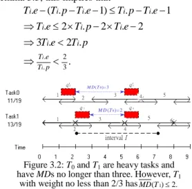
Figure 3.2: T

0

and T

1

are heavy tasks and have MDs no longer than three. However, T

1

with weight no less than 2/3 has

MD(T1)2.

In a word, when a task weight is at least 2/3, there are no consecutive maximal windows. Therefore, for any two

window(Ti,k) Ti

1



 





i i

c p window(Ti,k-1)

1 ) ( 





 





i i

i LPF T

c p

1



 





i i

c p

Figure 3.1(b):Ti.p mod Ti.e 2 1

) ( . . 

 



 i

i

i LPFT

e T

p T

. 1 .

 



 e T

p T

i i 1

. .

 



 e T

p T

i i

consecutive quanta, the maximum distance between them is at most two slots, when S is a Pfair schedule.

For example, in Figure 3.2, since 1>wt(T

₁

) ≧ 2/3, the distance between these two quanta (say q

3

and q

4

) that are allocated to T

_1,3

and T

_1,4

is at most two slots. Besides, any two consecutive maximal windows must include two overlaps; hence, the maximum distance between q

₂

’and q

3

’ . is at most three when 2/3>wt(T

₀

)≧1/2.

By equation (4), (5) and Lemma 3.5, the estimation of maximum distance of T

_i

can be written as Corollary 3.6.

Corollary 3.6. (The estimation of MD(T_i

))

The estimation of maximum distance of task T

_i

can be rewritten as

1 ) ( ,

2

₃²

 wt T

i



 ) ( T

i

MD 3 ,

₂¹

 wt ( T

i

) 

₃²

  2

1 .

.  ( ⁱ)2, ⁱ. mod ⁱ. 1, 0 ( ⁱ)

e T

p

T LPFT Tp Te wtT

i i

  ^{( ) 1, . mod . 2, 0 ( )} 2^. 1 .

.  ⁱ  ^{i i}   ⁱ 

e T

p

T LPFT Tp Te wtT

i i

4. Schedulability Conditions for Supertasks

In this section, the basic properties are presented and the schedulability condition for supertasks is described. In the later section, some properties are used to determine which supertasks need to be merged or reweighted.

Definition 4.1. (wasted quanta) The quanta allocated to

supertask ST in time slot 

t

,

t

 1  , while none of its component tasks receive them.

Definition 4.2: (least common multiplier of task set τ)

LCM({ τ }) denotes the least common multiplier of all task periods T

_i

.p, where T

_i

τ .

The following three lemmas are rather technical in nature, and are used the machinery to prove Theorem 4.4.

Claim 4.1: Let S be a Pfair/EPDF schedule. Suppose time

interval I=[t, t+l] for t=0 or LCM({ τ }), l>0 and U ≦ M, then

TiLag₍S_,Ti_,I_)0.

Lemma 4.2. (wasted-quanta lemma)

Let wt(ST)=

CTST i

i

wt ( CT ) . Before the first deadline missing in its component task, it does not exist in any wasted quanta.

Proof: We give a proof by contradicting the lemma. Assume

that the first wasted quanta occurs at time slot 

t

^,

t

 ¹  ; that is, for all CT

_i

ST, Lag(S, CT

_i

, t)≦0 such that

. 0 ) , ,



( 

ST

CT i

i Lag SCT t

.

We now consider two cases:

Case 1:

_{ CT}

i

_{ ST , Lag ( S , CT}

i

_{, t )  0}

This implies that time t is the least common multiplier of all CT

_i

’ s periods, and thus the amount of supertask windows is equal to that of all component task windows within interval  0 , t



. Consequently, no deadline missing occurs before time t+1.

Case 2:

_{ CT}

i

_{ ST , Lag ( S , CT}

i

_{, t )  0}

When ST receives one quantum at slot  t , t  1  , given Pfair assumptions, the equation can be written as follows:



( , ) 0 . ( 7 )

) , (

0 ) , , (

,

0











j t S ST j t

ST Share

t ST S Lag

The assumption in case 2 can be written as

 

( , ) 0 . ( 8 ) )

, (

0 ) , , (

,

0









 





 





ST

CT j t i

ST

CT i

ST

CT i

i i

i

j CT S t

CT Share

t CT S Lag

Since wt(ST)= 

CTST i

i

wt ( CT ) ,

. ) , ( )

,

( 

 

ST

CT i

i Share CT t t

ST Share

The relationship between (7) and (8) can be expressed as,

( , ) ( , ).

, 0 ,

0 

     t j ST

CTi j tSCTi j S ST j

Because the integer assumption of time slots, the value of 

CTiST



j_0,jS

(

CTi

,

j

) is at least

_0,

( , )  1



j t S ST j

. Since the supertask lacks of one quantum, one of the component tasks misses its deadline in interval   0 ,

t

. This contradicts our assumption.

Case 3:

 CT

i

 ST , Lag ( S , CT

i

, t )  0

By Claim 4.1, this case does not exist. ■

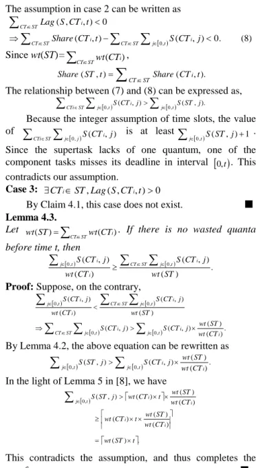
Lemma 4.3.

Let wt ( ST )  

_CTi_ST

wt ( CT

ⁱ

) . If there is no wasted quanta before time t, then

   

.

) (

) , ( )

( ) ,

(

0,

, 0

ST wt

j CT S CT

wt j CT

S CT ST j t i

i t

j i

i 





 

Proof: Suppose, on the contrary,

 

  .

) (

) ) ( , ( )

, (

) (

) , ( )

( ) , (

, 0 ,

0

, 0 ,

0

t i

j i

ST

CT j t i

ST

CT j t i

i t

j i

CT wt

ST j wt CT S j

CT S

ST wt

j CT S CT

wt j CT S

i

i











 

 





 

 



By Lemma 4.2, the above equation can be rewritten as

    .

) (

) ) ( , ( )

,

( 0,

,

0 j t i i

t

j wt CT

ST j wt CT S j

ST

S 







 

In the light of Lemma 5 in [8], we have



 



^{( )}



^. ) (

) ) (

(

) (

) ) (

( ) ,

, (

0

t ST wt

CT wt

ST t wt CT wt

CT wt

ST t wt CT wt j ST S

i i

i t i

j







 



 







 

This contradicts the assumption, and thus completes the

proof. ■

Making use of Lemma 4.3, we can prove the following schedulability condition easily.

ST

CT1

CT2

DEADLINE MISSED Within ST

4

t t10

Figure 4.1: The distance between quanta q

1

and q

2

is not shorter than ST.mcw, if the component tasks miss its deadlines.

q2

q1 MD(ST)= 5

ST.mcw = 5

Theorem 4.4. (The sufficient schedulability condition for

EPDF component tasks.)

For any supertask ST with EPDF-scheduled component task CT1, …, CT2,

wt

(

ST

)  

_CTi_STwt

(

CTⁱ

) , and schedule S is Pfair schedule. If MD(ST)<ST.mcw, then no deadline missing occurs at CT

_i

 ST.

Proof: In Fig.4.1, assume that the component task CT_i

misses its deadline at time t. We prove that the distance