電阻抗斷層掃描的一種最佳化-最小限度化演算法

(1)

國立臺灣大學理學院數學系博士論文

Department of Mathematics College of Science

National Taiwan University Doctoral Dissertation

電阻抗斷層掃描的一種最佳化-最小限度化演算法 A Majorization–Minimization Algorithm for

Electrical Impedance Tomography

劉于國 Yu-Guo Liu

指導教授：陳宜良博士 Advisor: I-Liang Chern, Ph.D.

中華民國 107 年 7 月 July, 2018

(2)

(3)

誌謝

我感謝姜明老師，陳宜良老師，和口試委員們對此篇論文提供背景知識及建議。我的摯愛璟琳和摯友家賢，感謝你們無條件的支持。感謝我的爸媽，我將此篇文章獻給你們。

(4)

(5)

Acknowledgements

I am glad to thank Dr. Ming Jiang, Dr. I-Liang Chern, and oral defense committee members for providing background knowledges and suggestions for this paper. I thank to my dear love Jing-Lin Li and my dear friend Mazer Lin, you are very supportive. Thank to my parents, I dedicate this paper to you.

(6)

(7)

摘要

本論文對電阻抗斷層掃描協同一普遍類型的非光滑正則提出了一統整的最佳化-最小限度化 (MM) 演算法，其中包含了稀疏與總變差正則。我們證明此提出之 MM 演算法的全域收斂性，且呈現源自模擬數據的數值重建結果。此 MM 演算法的數值結果顯示了對目標能量的快速遞減及對內含物的強度和位置有好的估計。此外，我們比較此 MM 演算法和廣為所用的高斯-牛頓法，此 MM 演算法對模擬導電率有較好的逼近。

關鍵字：電阻抗斷層掃描, 最佳化-最小限度化演算法

(8)

(9)

Abstract

In this paper, a unified majorization–minimization (MM) algorithm is proposed for electrical impedance tomography with a general type of nonsmooth convex regularization, including sparse and total variation regularizations.

We prove the global convergence of the proposed MM algorithm and show numerical reconstructions from simulated data. The numerical results of the MM algorithm show a fast decrease in objective energy and good estimates of the intensity and location of inclusions. Besides, we compare the MM algorithm to the widely used Gauss-Newton method, and the MM algorithm shows better approximation to the simulated conductivity.

Keywords: Electrical impedance tomography (EIT), majorization–-minimization (MM) algorithm.

(10)

(11)

List of Figures

3.1 An illustration of signal process for CEM-based EIT with electrodes on contact boundaries eℓdefined in (3.1), current injecting on e1, e2, and volt- age difference measured on e₅, e₆. . . 6 3.2 An illustration of Adjacent Method for the CEM-based EIT data acquisi-

tion with the measured data set{⟨

nqi, U (n_q^′

i)⟩

: i = 1, . . . , 13} defined in (3.4),(3.5). . . 7

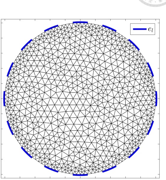
6.1 Conductivity distributions ς[T18230, s_p] : Ω_T₁₈₂₃₀ → R defined in (6.1) for FEM data simulation are shown in (b)–(e) with FEM domain Ω_T₁₈₂₃₀ shown in (a) and conductivity basis coefficient sp ∈ {0.5, 1, 1.5}¹⁸²³⁰. . . 28 6.2 FEM domain Ω_T₁₄₈₀ constructed by 1480 disjoint triangles for reconstruc-

tion is attached by 16 electrodes on contact boundaries e_l, l = 1, . . . , 16. . 29 6.3 The graphs of eF_p(10^y) defined in (6.12) are depicted by 101 uniformly

sampled points y_1,...,101 ∈ [−10, 10], and corresponding minimums are computed by GSS. . . 31 6.4 Least Square reconstructions using MM-CP algorithm with 2, 10, 50 itera-

tions from the 1% gaussian noise data g_pdefined in (6.5). Column one are simulated conductivity distributions defined in Figure 6.1; Column 2,3,4 are reconstructed ones with coefficient s^k_p,0 defined in (6.13) computing k-th iteration of MM-CP algorithm. . . . 33 6.5 Sparse reconstructions using MM-CP algorithm with 2, 10, 50 iterations

from the 1% gaussian noise data g_p defined in (6.5). Illustrations are the same as in Figure 6.4. . . 34

(14)

6.6 TV reconstructions using MM-CP algorithm with 2, 10, 50 iterations from the 1% gaussian noise data g_p defined in (6.5). Illustrations are the same as in Figure 6.4. . . 35 6.7 Least Square reconstructions using MM-CP algorithm with 50 iterations

from the 1% gaussian noise data g_pdefined in (6.5). Column one are simulated conductivity distributionsDp defined in Figure 6.1; Column two are reconstructed onesRp with coefficient s⁵⁰_p,0 defined in (6.13) computing 50-th iteration of MM-CP algorithm. We compareDp,Rp in last two columns by uniformly sampling 100 points on Γ_1,2 defined on top. . . 36 6.8 Sparse reconstructions using MM-CP algorithm with 50 iterations from

the 1% gaussian noise data g_p defined in (6.5). Illustrations are the same as in Figure 6.7. . . 37 6.9 TV reconstructions using MM-CP algorithm with 50 iterations from the

1% gaussian noise data g_pdefined in (6.5). Illustrations are the same as in Figure 6.7. . . 38 6.10 Comparison of least square, sparse , TV reconstructions using MM-CP

algorithm with 50 iterations from the 1% gaussian noise data g_p defined in (6.5). We show simulated conductivity in column one, and show least square, sparse , TV reconstructions in column 2,3,4, respectively. . . 39 6.11 Energy E_p,a(s^k_p,a) for least square, sparse, TV reconstructions are shown

in (a),(b),(c) respectively. . . 40 6.12 Comparison of the simulated and reconstructed conductivity distributions.

First column: simulated distributions. Second and third columns: Sparse and TV reconstructed distributions using the MM-CP algorithm, respectively. Fourth and fifth columns: Sparse and TV reconstructed distributions using the GN method, respectively. . . 42 6.13 Comparison with the energy decrease of the MM algorithm and GN method. 42

(15)

List of Tables

6.1 Estimate of background conductivity, contact impedance . . . 31 6.2 Error estimates of the reconstructed conductivities using the MM-CP al-

gorithm and the Gauss-Newton method with β = 10⁻⁶. . . 43 6.3 Error estimates of the reconstructed conductivities using the GN method

with smooth parameters β = 10⁻³, 10⁻⁹. . . 43

(16)

(17)

Chapter 1 Introduction

Electrical impedance tomography (EIT) is a signal to image process in which we estimate the conductivity distribution of an object by injecting currents and measuring voltages from its boundary. This process is a nonlinear, ill-posed inverse problem; thus, a direct formula is unavailable. However, the least-squares reconstruction with some regularizations are viable, such as Tikhonov regularization [26], sparse regularization [9], and total variation (TV) regularization [4].

In this paper, we focus on solving the regularization problem of complete electrode model (CEM)-based EIT [25]. In the case of smooth regularizations, Gauss–Newton type methods [17, (2.25)] are widely used, e.g., see [19] for Tikhonov regularization with level set representation of conductivity distributions and see [4],[10],[11] for smoothed TV regularizations. In the case of non-smooth regularizations, Monte Carlo sampling methods were discussed in [17] for sparse and TV regularizations, and an iterative soft shrinkage- type algorithm was proposed in [9] for sparse regularization. However, in the regularization problem of CEM-based EIT, an iterative method for both sparse and TV regularizations with global convergence to a critical point is rarely discussed.

We propose a unified majorization–minimization (MM) algorithm [15] for CEM-based EIT with a general type of nonsmooth convex regularization, including sparse and TV regularizations. The MM algorithm is an iterative method that monotonically decreases the objective energy by minimizing an appropriate chosen majorizer [15, (1)]. The majorizer we propose is based on the monotonicity relation [13, Lemma 2.1], which is a kind of

(18)

squeeze theory for elliptic partial differential equations and was used in CEM-based EIT for shape reconstruction [8, (5)] and resolution guarantees [14, Thm 2]. In addition to those applications of the monotonicity relation, we show that it can be used in CEM-based EIT for developing a globally convergent MM algorithm.

With regard to the computational efficiency of MM algorithms, the main cost is the majorizer–minimizing step. Due to the convexity of the proposed majorizer, in the minimization step, we can apply the Chambolle-Pock (CP) algorithm [6, (38)], which is a gen- eral uniformly convex optimization solver with a convergence rate of O(1/k²) [6, Thm 2].

The organization of the paper is as follows. In Chapter 2 we introduce the general subgradient for defining the critical point, function spaces for proving global convergence, , MM definition and related operators for computations. Finally, we introduce matrix nota- tions for describing the regularization problem. In Chapter 3, we give the problem formu- lation for CEM-based EIT. In Chapter 4, we describe the main regularization problem in this paper and develop the MM algorithm based on the monotonicity relation. In Chapter 5, we cast the MM algorithm into a framework of uniformly convex optimization that can be solved by O(1/k²) CP algorithm and then results in the MM-CP algorithm. In Ap- pendices,we prove the propositions and formulas used in MM-CP algorithm. We show the numerical results in Chapter 6, discuss relevant results in Chapter 7, and conclude the paper in Chapter 8.

(19)

Chapter 2 preliminary

For classes of differentiable functions, by referring to [20, §1.2.2], we denote by C_L^1,1(U ) the class of functions f :Rⁿ→ (−∞, ∞] that are continuously differentiable on U ⊂ Rⁿ and satisfy|f(x)|, ∥∇f(x)∥, ∥∇f(x) − ∇f(y)∥/∥x − y∥ ≤ L for all x, y ∈ U, x ̸= y.

In variation analysis [23], for f : Rⁿ → (−∞, ∞], we define dom f = {x ∈ Rⁿ : f (x) < ∞}. For x ∈ dom f, we define b∂f(x) = {v : f(y) ≥ f(x) + ⟨v, y − x⟩ + o(|y − x|)} to be the regular subgradient of f at x, and we define ∂f(x) = {v : ∃ xⁿ → x, vⁿ→ v with f(xⁿ)→ f(x), vⁿ∈ b∂f(xⁿ)} to be the general subgradient of f at x. For f ∈ C_L^1,1(U ), we have ∂f (x) = ∇f(x) for x ∈ U [23, Exer 8.8(b)]. In general, we say x is a critical point of f if 0∈ ∂f(x) [2, (1)].

In convex analysis [3], we denote Γ₀(Rⁿ) to be the set of lower semicontinuous convex function f : Rⁿ → (−∞, ∞] with dom f ̸= ∅. For J ∈ Γ0(Rⁿ), we have ∂J (x) = {p : J(y) ≥ J(x) + ⟨p, y − x⟩} [23, Prop 8.12]. The indicator function IE, defined by IE(x) = 0 if x∈ E and IE(x) =∞ if x ∈ Rⁿ− E, belongs to Γ0(Rⁿ) if E is closed and convex.

For the MM algorithm, by referring to [15], we say a family of functions {f^y}y∈Y

(uniformly) majorizes f if f^y(x)≥ f(x), f^y(y) = f (y), f^y ∈ Γ0(Rⁿ)∀ y ∈ Y ⊂ Rⁿ, x∈ Rⁿ(and∃γ > 0, f^y(y^′)≥ f(y^′) + γ∥y^′− y∥²∀ y, y^′ ∈ Y ). We call such family {f^y}y∈Y

a majorizer of f . By contrast, we say{f^y}y∈Y minorizes f if{−f^y}y∈Y majorizes−f.

Then, we say y^k+1 = argmin_y_∈Y f^y^k(y) is an MM algorithm for min_y_∈Y f (y) if{f^y}y∈Y

majorizes f . We define the proximity operator prox[f ](x) = argmin f (y) + ¹∥y − x∥²

(20)

and projection operator PE(x) = prox[IE](x) for computations.

In matrix notation, A ≻ 0 and A ≽ 0 denote that A is a real symmetric positive and a semi-positive definite matrix, respectively. For A ≻ 0, we define the inner product

⟨x, y⟩A = ⟨x, Ay⟩ and its norm ∥x∥A = √

⟨x, x⟩A. For K ∈ R^m,n, the matrix norm is defined by∥K∥ = max_∥x∥≤1∥Kx∥.

(21)

Chapter 3 Mathematical Modeling

Thus the highest form of generalship is to balk the enemy’s plans.

The Art of War by Sun Tzu - Chapter 3 : Attack by Stratagem

3.1 Complete Electrode Model

Given a domain Ω⊂ R^2,3and electrodes on e_ℓ⊂ ∂Ω with contact impedances zℓ > 0, ℓ = 1, . . . , L, the injecting current I and measured voltages U = U (I) on e_1,...,Lare supposed to satisfy the Complete Electrode Model (CEM) [27] :

−∇ · (ς∇u) = 0 in Ω u + z_ℓς∂u

∂ν = U_ℓ on e_ℓ, ℓ = 1, . . . , L

∫

eℓ

ς∂u

∂ν ds = I_ℓ for ℓ = 1, . . . , L ς∂u

∂ν = 0 on ∂Ω− ∪^Lℓ=1e_ℓ,

(3.1)

where ς ∈ L^∞+(Ω) = {f : s+ < f|Ω < M for some s₊, M > 0} is a conductivity distribution, and

U, I ∈ R^L_⋄ = {

y∈ R^L:

∑L

y_ℓ = 0 }

.

(22)

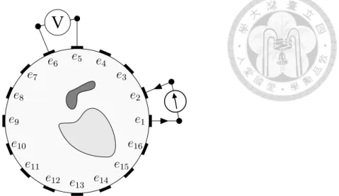
The signal process of CEM-based EIT is illustrated in Figure 3.1.

V

e₁ e₂ e₃ e₄ e₅ e₆ e₇ e₈ e₉

e10

e₁₁

e₁₂ e13 e₁₄ e₁₅

e16

Figure 3.1: An illustration of signal process for CEM-based EIT with electrodes on contact boundaries e_ℓdefined in (3.1), current injecting on e₁, e₂, and voltage difference measured on e5, e6.

For data acquisition we adopt the Adjacent Method that measuring the voltage difference on an adjacent electrode pair by injecting current on another adjacent electrode pair, see [18] for detail. Mathematically the measured data set for Adjacent Method can be formulated as

M = {⟨np, U (n_p′)⟩ | ⟨np, n_p′⟩ = 0; 1 ≤ p^′ < p≤ L}, (3.2)

where we set

n₁ = [1,−1, 0, . . . , 0]^t n2 = [0, 1,−1, 0, . . . , 0]^t n₃ = [0, 0, 1,−1, 0, . . . , 0]^t

...

nL−1 = [0, . . . , 0,−1, 1]^t n_L= [−1, 0, . . . , 0, 1]^t

(3.3)

and set p^′ < p to exclude symmetric data ⟨np^′, U (n_p)⟩ = ⟨np, U (n_p′)⟩ to be verified in (3.8). For example, ⟨n3, U (n₁)⟩ is the voltage difference on electrode pair 3-4 with injecting current on electrode pair 1-2. For example,⟨n3, U (n₁)⟩ is the voltage difference on electrode pairs 3-4 with injecting current on electrode pair 1-2.

(23)

From (3.2),(3.3) the total amount of measured data is m = L(L− 3)/2, then there exists sequences q_i, q^′_i, i = 1, . . . , m such that

M = {⟨

n_q_i, U (n_q′ i)⟩

: i = 1, . . . , m}. (3.4)

For example, if L = 16 we can choose

(q1, q^′₁) = (3, 1), ...

(q₁₃, q₁₃^′ ) = (15, 1), (q14, q₁₄^′ ) = (4, 2),

...

(q₁₀₄, q₁₀₄^′ ) = (16, 14)

(3.5)

and we show the data set{⟨

n_q_i, U (n_q′ i)⟩

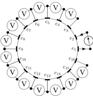
: i = 1, . . . , 13} in Figure 3.2. Next, we simulate M in (3.4) by the finite element method (FEM) [27].

V V V V

V V V

V

V V V V V

e₁ e₂ e₃ e4

e₅ e6

e₇ e₈ e₉

e₁₀ e₁₁

e12 e₁₃ e14

e₁₅ e₁₆

Figure 3.2: An illustration of Adjacent Method for the CEM-based EIT data acquisition with the measured data set{⟨

nqi, U (n_q′ i)⟩

: i = 1, . . . , 13} defined in (3.4),(3.5).

(24)

3.2 Finite Element Method based Model

In [25], the solution of (3.1) (u, U ) = (u, U )(I)∈ H = H¹(Ω)⊕ R^L_⋄ is shown to satisfy

Vς((u, U ), (u^′, U^′)) =FI((u^′, U^′)) (3.6)

for all (u^′, U^′)∈ H, where H¹(Ω) is the Sobolev space and

Vς(·, ·) = Cς(·, ·) +

∑L ℓ=1

1

zℓBℓ(·, ·), FI((u^′, U^′)) =⟨I, U^′⟩

withCς(·, ·), Bℓ(·, ·) defined by

Cς((u, U ), (u^′, U^′)) =

∫

Ω

ς∇u · ∇u^′dx Bℓ((u, U ), (u^′, U^′)) =

∫

eℓ

(u− Ul)(u^′ − U_l^′) dS.

Then,∀ zℓ > 0, ς ∈ L^∞+(Ω), we have positivity

Bℓ(w, w)≥ 0, Cς(w, w)≥ 0, Vς(w, w) > 0 (3.7)

for all 0̸= w ∈ H and the symmetry

⟨n_q_i, U (n_q′ i)⟩

=Fn_qi((u, U )(n_q′ i))

=Vς((u, U )(n_q_i), (u, U )(n_q′ i))

=Vς((u, U )(n_q^′

i), (u, U )(nqi))

=Fn_q′

i

((u, U )(n_q_i)) =⟨ n_q′

i, U (n_q_i)⟩ .

(3.8)

In the FEM, we assume

Ω =

∪n j=1

△j (3.9)

is composed by the union of disjoint triangles (tetrahedrons)△1,...,ninR²(R³) over given

(25)

N nodes v... 1,...,...

N. Additionally, we assume

ς =

∑n j=1

sjχ_△_j, (u, U ) =

N =...

N +L−1

∑

k=1

akΦk, (3.10)

where χ_△_j are characteristic functions on△j and

Φ_k =









(ξk, 0) if k = 1, . . . ,...

N (0, nk−...

N) if k = ...

N + 1, . . . , N

with ξ_kbeing piecewise linear basis functions satisfying ξ_k(v_k′) = δ_kk′, which is the Kro- necker delta over index k, k^′ = 1, . . . ,...

N . By substituting (3.9) and (3.10) into (3.6) and by choosing (u^′, U^′) = Φ_kfor k = 1, . . . , N we have

V_sa = b(I), (3.11)

where

[V_s]_kk′ =V^∑ⁿ_j=1sjχ_△j(Φ_k, Φ_k′)

=

∑L ℓ=1

1

z_ℓBℓ(Φ_k, Φ_k′) +

∑n j=1

s_jCχ_△j(Φ_k, Φ_k′), [b(I)]_k =FI(Φ_k), for k, k^′ = 1, . . . , N.

Setting [B_ℓ]_kk′ =Bℓ(Φ_k, Φ_k′) and [C_j]_kk′ =Cχ_△j(Φ_k, Φ_k′), we have

V_s=

∑L ℓ=1

1 zℓ

B_ℓ+

∑n j=1

s_jCj.

With those equations and (3.7), we obtain

B_ℓ, C_j ≽ 0, Vs ≻ 0

for all s_j > 0, j = 1, . . . , n, ℓ = 1, . . . , L. Explicitly, we have

B_ℓ =



B_ℓ¹ B_ℓ² B_ℓ³ B_ℓ⁴



 , C^j =



A_j 0

0 0



, b(I) =



 0 F (I)





(26)

with [B_ℓ³] = [B_ℓ²]^tand

[A_j]_kk_′ =

∫

△j

∇ξk· ∇ξk^′dx, k, k^′ = 1, . . . ,...

N , [B_ℓ¹]_kk_′ =

∫

eℓ

ξ_kξ_k′dS, k, k^′ = 1, . . . ,...

N , [B_ℓ²]_kp =−[np]_ℓ

∫

eℓ

ξ_kdS, k = 1, . . . ,...

N , p = 1, . . . , L− 1, [B_ℓ⁴]_pp_′ =|eℓ| [np]_ℓ[n_p′]_ℓ, p, p^′ = 1, . . . , L− 1,

F_p(I) = ⟨I, np⟩ , p = 1, . . . , L − 1.

According to (3.10) and (3.11), we assume (u, U )(n_q^′

i) = ∑N

k=1αkΦk with Vsα = b(n_q′

i). Then, by (3.8), we have

⟨n_q_i, U (n_q′ i)⟩

=Fn_qi((u, U )(n_q′

i)) =Fn_qi(

∑N k=1

α_kΦ_k)

=

∑N k=1

α_kFn_qi(Φ_k) =⟨α, b(nqi)⟩ =⟨

b(n_q_i), b(n_q^′

i)⟩

Vs⁻¹,

by which (3.4) becomes

M = {⟨ϕi, ϕ^′_i⟩_V_s⁻¹ : i = 1, . . . , m} (3.12)

with ϕ_i = b(n_q_i), ϕ^′_i = b(n_q′ i).

3.3 Reconstruction using Regularization Problems

From (3.12), we define the coefficients-to-data mapping

f_i(s) =⟨ϕi, ϕ^′_i⟩_V_s⁻¹, i = 1, . . . , m

with dom f_i = [s₊,∞)ⁿfor some s₊ > 0. Then, we formulate the regularization problem of CEM-based EIT as

mins∈E E(s), (3.13)

(27)

where

E(s) = ϵJ (s) + F(s), F(s) = 1

2∥f(s) − g∥²

being with given measured data g, a box constraint E⊂ [s+,∞)ⁿ, regularization param- eter ϵ, and the regularization function J , which is discussed next.

For the regularization J used in CEM-based EIT, by referring to [17, (4.5),(4.7)], we define the zero function J₀, the sparse regularization J₁, and total variation J₂by

J₀(ς) = 0, J₁(ς) =∥ς − s^∗∥L¹(Ω), J₂(ς) =

∫

Ω

|∇ς| dx

with s^∗ ∈ R being a precalculated background conductivity discussed in Chapter 6.2.

Then by (3.10) we have

J₁(ς) =

∑n j=1

|sj − s^∗| |△j|

and

J₂(ς) = 1 2

∑n i,j=1

|si− sj| |∂△i∩ ∂△j|

=

∑κ k=1

|stk − st^′_k| |∂△tk ∩ ∂△t^′_k|

for some subsequence t_k, t^′_ksuch that|∂△tk∩∂△t^′_k| > 0 and tk ̸= t^′_k∀ k = 1, . . . , κ. That implies

J1(ς) =∥C1(s− s^∗I)∥1, J2(ς) =∥C2s∥1

withI represents all 1 vector, C1 ∈ Rⁿ^×ndefined by

C₁ = diag(|△1|, . . . , |△n|)

and C2 ∈ R^κ^×ndefined by

[C₂]_kl=











|∂△tk∩ ∂△t^′_k| if l = t_k

−|∂△tk∩ ∂△t^′_k| if l = t^′_k 0 if l̸= tk, t^′_k.

(28)

Then, J0,1,2are in the form of

J_a = J_a(s, s^∗) =∥Ca(s− da(s^∗))∥1, a = 0, 1, 2 (3.14)

with d0(s^∗) = d2(s^∗)∈ {0}ⁿ, d1(s^∗)∈ {s^∗}ⁿ, and C0being the zero matrix.

As pointed in Chapter 1, the Gauss-Newton type method [17, (2.25)] with a line search is widely used for solving smooth regularization problem of CEM-based EIT. Numerically for solving (3.13) the Gauss-Newton type method with line search iterates as

s^k+1 =Aσ(s^k) := s^k− σ(ϵ∇²J (s^k) + f^′(s^k)^tf^′(s^k))⁻¹∇E(s^k),

with f^′(s) :Rⁿ → R^mdefined by f^′(s)_ij = (∇fi(s))_j and

σ = argmin

σ^′>0

E(Aσ^′(s^k))

computed by line search method [5, (9.16)].

For solving non-smooth regularization problem of CEM-based EIT an iterative soft shrinkage-type algorithm proposed in [9] for sparse regularization J₁is based on the proximity (see Preliminary) type algorithm proposed in [28] that solves (3.13) by

s^k+1=Bσ(s^k) := prox_σϵJ₁(s^k− σ∇F(s^k)),

for some σ > 0 satisfying

E(Bσ(s^k))≤ max

max{k−5,0}<k^′≤kE(s^k^′)− 10⁻⁵σ∥Bσ(s^k)− s^k∥² that ensures accumulation points of{s^k}k∈Nare critical points of E.

To sum up, a numerical method for solving the non-smooth regularization problem of CEM-based EIT with global convergence to a critical point is rarely discussed. In this paper, we propose a Majorization-Minimization (MM) algorithm (see Preliminary) to solve the non-smooth regularization problem of CEM-based EIT with regularizations of

(29)

the form (3.14) including sparse, TV regularizations. We prove the global convergence of proposed MM algorithm and show numerical results from simulated data next.

(30)

(31)

Chapter 4 A Majorizaton-Minimization Algorithm

Based on the finite element method (FEM) [27], it is shown in Chapter 3 that the regularization problem of CEM-based EIT can be formulated as Problem 1.

Problem 1. Given g ∈ R^m, ϵ > 0, f : Rⁿ → (−∞, ∞]^m, J ∈ Γ0(Rⁿ) and E ⊂ Rⁿ, we solve

mins∈EϵJ (s) + 1

2∥f(s) − g∥² that satisfies∀ i = 1, . . . , m,

• dom f_i = [s₊,∞)ⁿ, E = [s, s]ⁿ, 0 < s₊< s < s.

• fi(s) =⟨ϕi, ϕ^′_i⟩_V_s⁻¹for some ϕi, ϕ^′_i ∈ R^N, where Vs =∑L ℓ=1

1

zℓBℓ+∑n j=1sjCj

for some B_ℓ, C_j ≽ 0, zℓ > 0 such that V_s≻ 0 ∀ sj > 0.

• J (s) =∥C(s − d)∥1for some matrix C and vector d.

In Problem 1, g, ϵ, and J are the measured data, regularization parameter, and reg- ularization function, respectively. f is the conductivity-to-data mapping, in which the ϕ_i and ϕ^′_i represent the i-th voltage measuring and current injecting vector, respectively.

V_s, B_ℓ, C_j are the associated FEM matrices, and z_ℓ is the contact impedance between the object and the ℓ-th electrode. Finally, ∥C(s − d)∥1 is a general form representing the sparse or TV regularization.

(32)

We use Proposition 1 to construct a majorizer to develop an MM algorithm for Problem 1.

Proposition 1. Under the assumptions in Problem 1, for s, t ∈ (0, ∞)ⁿ, we denote

t s

2∈ (0, ∞)ⁿwith element t²_j/s_j, and for φ∈ R^N, we defineGφ : (0,∞)ⁿ→ R by

Gφ(s) =∥φ∥²_V−1 s . Then, for all s, t∈ (0, ∞)ⁿ, φ∈ R^N, we have

(a) (∇Gφ(s))_j =− ⟨Vs⁻¹φ, C_jV_s⁻¹φ⟩ ≤ 0.

(b) Gφ ∈ C_L^1,1(E) for some L > 0.

(c) Gφ(s)≥ Gφ(t) +⟨∇Gφ(t), s− t⟩.

(d) Gφ(s)≤ Gφ(t)− ⟨∇Gφ(t),t s

2− t⟩.

We prove Proposition 1 in Appendix A and refer Proposition 1(c)(d) to a vector version of the monotonicity relation [13, Lemma 2.1]. Observe in Problem 1 and Proposition 1 that

f_i(s) =⟨ϕi, ϕ^′_i⟩_V_s⁻¹ = 1 4

(Gϕi+ϕ^′_i(s)− Gϕi−ϕ^′i(s))

, (4.1)

by which and Proposition 1(c)(d) we have

f_i(t) +1 4

⟨∇Gϕi+ϕ^′_i(t), s− t⟩ +1

4⟨∇Gϕi−ϕ^′i(t),t s

2− t⟩

≤fi(s) (4.2)

≤fi(t)− 1 4

⟨∇Gϕi−ϕ^′i(t), s− t⟩

− 1

4⟨∇Gϕi+ϕ^′_i(t), t s

2− t⟩.

Then, for each t∈ E, by (∇Gφ(t))_j ≤ 0 (Proposition 1(a)), we construct a convex (con- cave) function that is greater (less) than f_i(s) in (4.2), which results in the following MM algorithm (4.3) for Problem 1.

(33)

Proposition 2. Under the assumptions in Problem 1 and Proposition 1, for t∈ E, i = 1, . . . , m, we define

ψ_i = ϕ_i+ ϕ^′_i, θ_i = ϕ_i− ϕ^′i, h^t_i(s) = f_i(t)− gi− 1

4⟨∇Gθi(t), s− t⟩ − 1

4⟨∇Gψi(t), t s

2− t⟩,

l^t_i(s) = f_i(t)− gi+1

4⟨∇Gψi(t), s− t⟩ +1

4⟨∇Gθi(t),t s

2− t⟩,

H_i^t(s) = max{h^t_i(s),−l^t_i(s)}, D^t(s) = 1 2∥s − t

s

2∥²

with dom h^t_i = dom − li^t= dom D^t= [s+,∞)ⁿ. Then, (a) {D^t}t∈Euniformly majorizes 0∀ i = 1, . . . , m.

(b) {Hi^t}t∈Emajorizes|fi− gi| ∀ i = 1, . . . , m.

(c) ∀ δ, ϵ > 0, s⁰ ∈ E,

s^k+1 = argmin

s∈E δD^s^k(s) + ϵJ (s) +1

2∥H^s^k(s)∥² (4.3)

converges to a critical point ofIE + ϵJ + ¹₂∥f − g∥².

We prove Proposition 2 in Appendix B and relate MM algorithm (4.3) to the proximity (see Preliminary) iteration

s^k+1 = argmin

s∈E

δ

2∥s − s^k∥²+ ϵJ (s) +1

2∥f(s) − g∥²

= prox [

IE+ ϵ δJ + 1

2δ∥f − g∥² ]

(s^k),

where ¹₂∥s − s^k∥²,∥f(s) − g∥² are replaced by majorizers D^s^k(s),∥H^s^k(s)∥²in (4.3).

By definition of (uniformly) majorization in Preliminary and Proposition 2(b) we have

(34)

{(Hi^t)²}t∈E majorizes (fi − gi)², by which and Proposition 2(a) we have {

δD^t+ ϵJ +1 2∥H^t∥²

}

t∈E

uniformly majorizes ϵJ + 1

2∥ bf− g∥²

for all δ, ϵ > 0. That confirms that (4.3) is an MM algorithm for Problem 1; moreover, it is a sequence of convex optimization problems. Thus, an efficient numerical solver is critical and is discussed next.

(35)

Chapter 5 The Computation

For the computation of (4.3), we use the O(1/k²) CP algorithm that is proposed to solve the saddle point problem

min

x∈R^M max

y∈R^{M ′}⟨Kx, y⟩ + G(x) − F (y) (5.1) by the following iteration











y^k+1 = prox[σ_kF ](y^k+ σ_kK ¯x^k) x^k+1 = prox[τ_kG](x^k− τkK^ty^k+1) θ_k= 1/√

1 + 2γτ_k, τ_k+1 = θ_kτ_k, σ_k+1 = σ_k/θ_k

¯

x^k+1 = x^k+1+ θ_k(x^k+1− x^k)

. (5.2)

In (5.1), it assumes that K ∈ R^M^′^×M, F ∈ Γ0(R^M^′), and G is uniformly convex with parameter γ > 0 (used in (5.2)), i.e.,

G(x^′)≥ G(x) + ⟨∂G(x), x^′ − x⟩ +γ

2∥x^′− x∥² ∀ x^′, x∈ R^M.

In (5.2), the initializations are given by (x₀, y₀) ∈ R^M × R^M^′, ¯x₀ = x₀, and σ₀, τ₀ > 0 with σ₀τ₀∥K∥² ≤ 1.

To apply the CP algorithm, we transform (4.3) to the form of (5.1). Proposition 2(b)

(36)

implies H_i^t≥ |fi− g| ≥ 0, which implies

(H_i^t(s))² = (max{h^ti(s),−l^ti(s)})²

= min

r_i ∈ R h^t_i(s)≤ ri

−l^ti(s)≤ ri

r_i²

(5.3)

for i = 1, . . . , m. Then, by (5.3), iteration (4.3) becomes

s^k+1 = argmin

s∈ E D^s^k(s) + ϵ

δJ (s) + 1

2δ∥H^s^k(s)∥²

= argmin s∈ E h^s^k(s)≤ r

−l^s^k(s)≤ r

∥s∥

2

+1 2∥(s^k)

s

2

∥²+ ϵ

δJ (s) +∥r∥

2δ

2

. (5.4)

We define A_k, B_k∈ R^m^×n, c^k₁, c^k₂ ∈ R^m, R_k ⊂ Rⁿ× Rⁿby











[A_k]_ij =(

−∇Gψi(s^k))

j/4 [B_k]_ij =(

−∇Gθi(s^k))

j/4 c^k₁ = f (s^k)− g − (Ak+ B_k)s^k c^k₂ = g− f(s^k)− (Ak+ B_k)s^k R_k ={(s, t) ∈ Rⁿ× Rⁿ: s_jt_j ≥(

s^k_j)2

, s∈ E}.

(5.5)

Then, we have

h^s^k(s) = B_ks + A_k(s^k) s

2

+ c^k₁,

−l^s^k(s) = Aks + Bk

(s^k) s

2

+ c^k₂

(37)

for all s∈ E, and

s^k+1 = argmin s∈ E

Bks + Akt + c^k₁ ≤ r A_ks + B_kt + c^k₂ ≤ r

t = (s^k) s

2

∥s∥

2

+ ∥t∥

2

+ ϵ

δJ (s) + ∥r∥

2δ

2

(5.6)

= argmin s∈ E

B_ks + A_kt + c^k₁ ≤ r A_ks + B_kt + c^k₂ ≤ r

t≥ (s^k) s

2

∥s∥

2

+ ∥t∥

2

+ ϵ

δJ (s) + ∥r∥

2δ

2

(5.7)

= argmin s

B_ks + A_kt + c^k₁ ≤ r A_ks + B_kt + c^k₂ ≤ r

(s, t)∈ Rk

∥s∥

2

+ ∥t∥

2

+ ϵ

δJ (s) + ∥r∥

2δ

2

, (5.8)

where (5.4)⇐⇒ (5.6) and (5.7) ⇐⇒ (5.8) because of (5.5) and (5.6) ⇐⇒ (5.7) because

∥t∥²,∥r∥², [A_k]_ij, [B_k]_ij ≥ 0 force (5.6) and (5.7) to share the same optimal (s, t).

Note that (5.8) is a uniformly convex optimization problem with constraints that clearly satisfies Slater’s condition [5, (5.26)]. Then, it is equivalent to solve (5.8) by the following saddle point interpretation [5, §5.4]:

s, t, rmin (s, t)∈ Rk

maxy, w y≥ 0 w∈ Qδ,ϵ

⟨B_ks + A_kt + c^k₁ − r, y1

⟩+

⟨A_ks + B_kt + c^k₂ − r, y2

⟩+

⟨w, C(s − d)⟩ + ∥(s, t)∥

2

+∥r∥

2δ

2

,

(5.9)

where y = (y₁, y₂)∈ R^m× R^m and

Q_δ,ϵ ={w : ∥w∥∞ ≤ ϵ } =[

−ϵ ,ϵ]

× · · · ×[

−ϵ , ϵ]

(5.10)

(38)

such that

ϵ

δJ (s) = ϵ

δ∥C(s − d)∥1 = max

w∈Qδ,ϵ

⟨w, C(s − d)⟩ .

Substitute r in (5.9) with the optimal value δ(y₁+ y₂) and define

T_δ(y) =I_{y≥0}(y) +δ

2∥y1+ y₂∥²

then, we reduce (5.9) to mins, t max

y, w

⟨B_ks + A_kt + c^k₁, y₁⟩ +

⟨A_ks + B_kt + c^k₂, y₂⟩

+⟨w, C(s − d)⟩ +

∥(s, t)∥

2

+IRk(s, t)− Tδ(y)− IQδ,ϵ(w).

(5.11)

By comparing (5.11) to (5.1), we have

K_k=







B_k A_k A_k B_k

C 0





 (5.12)

Gk(s, t) = 1

2∥(s, t)∥²+IR_k(s, t), F_k(y, w) = T_δ(y)−⟨

c^k, y⟩

+IQδ,ϵ(w) +⟨w, Cd⟩

corresponding to (K, G, F^∗) in (5.1) with G_k(s, t) is uniformly convex with parameter 1.

Then the substitution of K_k, G_k, F_k^∗ into (5.2) results in Algorithm 1 that computes s^kin (4.3) by MM-CP(s⁰, k, l_max, C, d, g, δ, ϵ), where s⁰ ∈ E is the initial conductivity and lmax