一個用於無線感測網路之延遲需求與節省能源耗用的折衷MAC通訊協定

(1)

國立臺灣大學電機資訊學院資訊工程研究所碩士論文

Department Computer Science and Information Engineering College of Electrical Engineer and Computer Science

National Taiwan University Master Thesis

一個用於無線感測網路之延遲需求與節省能源耗用的折衷 MAC 通訊協定

A Latency-Energy Trade-off MAC Protocol for Wireless Sensor Networks

李昂熹 Ang-Hsi Lee

指導教授：高成炎博士

Advisor: Prof., Cheng-Yan Kao, Ph.D.

中華民國 97 年 7月

July, 2008

(2)

(3)

Acknowledgement

這篇論文的完成，要歸功於許多人的幫忙與協助。首先要感謝指導教授高成炎教授，在研究所的這段時間，讓我能妥善分配時間於想鑽研的知識。接著要感謝的是金明輝學長，自從我進入實驗室之後，無論是在學業或是生活上皆對我循循善誘，指導我的研究，幫忙修正我的論文，給予了我相當大的幫助。如果沒有金學長的幫助，我的論文及口試也不會這麼順利完成。詹鎮熊學長平日對於我的研究也有諸多幫忙，對於我研究內容的建議也有非常大的裨益。口試時諸位口試委員提出了相當寶貴的建議，讓我更進一步地改善論文。感謝實驗室的所有同學：維志、麒瑋、孟家、子翔、歷新。在實驗室的這段期間，彼此互相提攜勉勵，有困難時大家也都鼓勵我，對於這段經歷，我永遠不會忘記。除此之外，還要感謝我的家人，在生活上協助我，讓我不用為了日常瑣事煩惱。在我遇到挫折時，持續的關心，那是我往前邁進的最大動力。這篇論文實在不是一個人所能完成的，謹以此文獻給諸多幫助我的人。

(4)

摘要

節省能源消耗一向是無線感測網路上最重要也最熱門的議題之一。這篇論文將介紹一個應用於無線感測網路上之媒體控制通訊協定： Latency MAC (LMAC)。我們首先將探討造成無線感測網路影響能源有效使用之各種因素，並藉由檢視無線感測網路的封包延遲時間需求，接著再尋找節省能源與封包延遲時間中的折衷方案。透過犧牲多餘的封包延遲時間來避免最大的能源浪費：閒置聽取。在這尋求折衷的過程之中，我們會遇到許多限制，因此，我們也必須一併研究及分析這些額外的限制因素，在這條件下設法達到一最佳的節省能源與封包延遲時間的折衷方案。藉由提升猜測資料封包的產生及傳輸時間預測準確率，我

們在模擬結果上發現LMAC 確實消耗了較少的能源，尤其是在一個鬆散封包延遲

時間或是較低網路傳輸的無線網路下。

(5)

ABSTRACT

This paper proposes Latency MAC (LMAC) protocol for wireless sensor networks.

We investigate the idle listening problem and try to avoid it by sacrificing latency. We examine the latency constraint in wireless sensor networks and study the tradeoff between extra latency and energy efficiency. In the process of trading latency for energy efficiency, there are many restrictions. Thus, we study and analyze these limitations and then try to achieve the best tradeoff between latency and energy-efficiency under these limitations. By increasing the arrival prediction accuracy of data packets, the simulation results show that LMAC indeed consumes less energy, especially under a loose latency constraint or a light traffic load in wireless sensor network environments.

(6)

LIST OF FIGURES

Figure 1. Listening State of MAC Protocols 10

Figure 2. Sleep and wake-up states of sensor nodes in LMAC 13

Figure 3. Contents of Time Slot 15

Figure 4(a). Arrival Rate 19

Figure 4(b). Initial Bulk parameters 19

Figure 4(c). Initial Doze parameters 19

Figure 4(d). Schedule fits Latency Constraint 19

Figure 5. Total energy consumption under different numbers of sensor nodes 24 Figure 6. Total energy consumption under different numbers of sensor nodes

& Source Nodes on Edge 24

Figure 7. Energy consumption of the busiest sensor node under different numbers

of sensor nodes 25

Figure 8. Total energy consumption under different arrival rates 25 Figure 9. Total energy consumption under different arrival rates

& Source nodes on edge 26

Figure 10. Energy consumption of the busiest sensor node under different arrival

rates 26

Figure 11. Total energy consumption under different latency constraint 27 Figure 12. States of latency constraint failures 27

(9)

LIST OF FORMULA AND TABLE

Formula (1) Transmission Rate Bounding 16

Formula (2) Remain Buffer Size 16

Formula (3) Probability of Buffer Overflowing 16

Formula (4) Expected Latency 17

Formula (5) The Worst Case Latency 17

Formula (6) Relation between Bulk and Doze 17

Table 1. Action of Node i at Time T 14

Table 2. Simulation Setup Parameters 22

Table 3. Extra energy consumption compared to LMAC

under different numbers of nodes 28

Table 4. Average Energy Consumption per packet

under different arrival rates 28

(10)

CHPATER 1

INTRODUCTION

A wireless sensor network is a comprised of large number of low-cost, low-energy, and multifunctional sensor nodes that are short in transmission range and operated by battery. Sensor nodes are usually distributed over an area where observers want to collect information. Their main functions are to sense data, to process data, and to communicate with the server. Wireless sensor networks are used in various applications such as environment monitoring, animal behavior tracking, factory controlling, homeland security, smart space developing, military detecting, human-health caring, etc.

Some features of wireless sensor networks are different from those of ad hoc networks.

For example, the number of sensor nodes in a wireless sensor network can be several times larger than that in an ad hoc network. Because the sensor nodes are low-cost and battery operated, they are prone to failure. Unlike nodes in ad hoc networks, sensor nodes in wireless sensor networks require more reliable fault-tolerant scheme. Data flow direction and energy constraints are the major difference between wireless sensor networks and traditional ad hoc networks. In wireless sensor networks, there are some special nodes which are called sinks. Sinks are the destinations of data packets and every sensor node will transmit the sensed data to the sink. Thus, the data flow in wireless sensor networks is generally one-way traffic to sinks from all sensor nodes except some protocol control data packets or communications occurred between sensor nodes, unlike the data flow which is point-to-point based in most of ad hoc networks.

Due to this communication direction characteristic, in a protocol design, most resources should be allocated to only one communication direction in wireless sensor networks.

(11)

Energy-efficiency is a critical issue in all wireless networks, especially in wireless sensor networks where sensor nodes are usually operated by battery in cheaper hardware devices and will not be maintained for a long time after the network topology is established. Furthermore, some sensor nodes are designed to be used once only because the locations of sensor nodes may be in an unreachable area.

1.1 Motivation

In general, wireless sensor networks demand a longer life time protocol than that of other wireless networks. Energy is the most critical constraint in most wireless sensor networks. The other constraints such as data latency and transmission rate are less concerned. Therefore, we try to enhance energy-efficiency by sacrificing these less important factors. The latency constraint vary in different application orientations of wireless sensor networks. For example, in a weather data sensing system, the temperature data refreshes each minute, the tide condition reports renew every thirty minutes, and the accumulated rain amount data collects each hour. The latency constraint in such applications can almost be ignored because the normal latency of a wireless network is less than a few seconds. The sensors are usually developed on buoy and very difficult to maintain in a tide condition monitoring system. In this case, we can focus on energy efficiency problem and forget the latency constraint completely.

However, in a human-health caring system, no matter how long the sensing frequency is, the sensed data must be transmitted to the server immediately. Thus, a sensor reports the emergency signal too slowly is not different from a broken sensor. That is to say, the latency allowance for the human-health caring system is very tight and is as important as energy-efficiency.

(12)

Due to the various constraints in different sensor network applications, designing a MAC protocol for wireless sensor networks which always achieves the lowest latency is not the best policy. In wireless sensor network environments, most protocols are designed for special purposes to fit some specific features. So we try to design a MAC protocol to reduce the energy wastage via sacrificing the extra latency under the latency constraint. While designing such a latency constraint fit protocol, there are many other restrictions in various wireless sensor networks to be considered, such as limited buffer size, tight latency constraint, low transmission rate, short transmission range, and so on.

In this thesis, although the key point we focus on is the trade-off between latency constraint and energy-efficiency, we have to take the other restrictions into consideration because we find that these restrictions cause the system to fail while we discard latency to improve the energy-efficiency.

1.2 Energy-Efficiency Problems in Wireless Sensor Networks

Because of some special topology architectures and critical energy-efficiency constraint in wireless sensor networks, most of the popular ad hoc network protocols like IEEE802.11 can not be used in wireless sensor networks. There are many various wireless sensor network-oriented protocols developed, such as hardware devices wake- up radio[6], energy-efficiency MAC protocols [2, 10, 12, 14], and energy-efficiency routing protocols [1, 9], etc.

There are some major energy wastage problems in wireless sensor networks. The first problem is idle listening. While a node is waiting and listening for possible incoming packets, the energy is wasted when there is no such packet. Idle listening problem is the main energy wastage in wireless networks. The second one is overhearing. When a sensor node receives a packet which does not belong to it, the

(13)

energy is also wasted. The third problem is control packet overhead. Some protocols will request nodes exchange information periodically to maintain the schedule scheme or topology. The control packets flowing in sensor nodes will increase energy consumption too.

Another energy-efficiency problem in wireless sensor networks is unbalanced consumption of energy. That is, the nodes that are closer to the sink nodes will be busier than other nodes. Therefore, their energy consumption will be heavier than others.

Actually, there is one more energy inefficiency problem: collision. But in current research, most of wireless network protocols use the RTS/CTS scheme [7] so the collision effect has been minimized.

There are two major directions of MAC protocol design in wireless networks:

contention based and TDMA based protocols [12]. Contention based protocols like IEEE 802.11, whose major energy wastage source is idle listening due to the uncertainty of when the packets will arrive, have to be aware of the network condition to gain the access right of transmission. This energy wastage is very difficult to overcome in this kind of design. In addition, contention based protocol will also cause the problem of overhearing because they will keep accessing the medium and receive all the neighboring packets or control packets nearby.

In TDMA based protocols, every sensor node’s wake-up and sleep time are scheduled. The sensor nodes will periodically operate their schedules. The schedules are usually generated by some specific algorithms in order to wake up a sensor node at the time that a packet comes, i.e., the sensor node will try to carrier sense at the possible data packets incoming time. The major energy inefficiency of TDMA based protocols results from idle listening and control packet overhead. The idle listening energy wastage is caused by missing predictions. Predictions can not be prefect no matter how

(14)

precise a protocol is. In additional, sensor nodes of a TDMA based MAC protocol have to keep exchanging control packets to maintain their schedule synchronized or to schedule online. These control packets will also increase the energy wastage.

This thesis presents Latency MAC (LMAC). In order to increase the energy- efficiency, we sacrifice some packet latency to reduce the energy wastage from idle listening, and to increase the accuracy of the prediction for packets incoming. As a result, Latency MAC can greatly reduce the energy wastage from idle listening in a loose latency constraint or in low arrival rate environment setups. In this thesis, we propose a new sleep schedule scheme for wireless sensor networks. This schedule reduces the energy wastage caused by idle listening. We also study the restrictions while trading latency to energy-efficiency and we figure out the bounds to latency trade-off.

1.3 Thesis Organization

In chapter 1, we introduce the background of wireless sensor networks and describe the energy inefficient problems in wireless networks. In chapter 2, we will introduce some energy-efficiency and latency-related MAC protocols and describe their advantages and disadvantages. In chapter 3, we will describe the overview and the details of LMAC principles. In this section, we will discuss the arrival rate factor, restrictions we encounter while designing the LMAC, and how we take them into consideration and solve them. In chapter 4, we will simulate LMAC and other energy- efficiency MAC protocols on NS2. Besides, we will compare LMAC with SMAC and PMAC on different metrics. In chapter 5, we will reach a conclusion and discuss the future work.

(15)

CHPATER 2

RELATED WORK

2.1 Energy-Efficiency MAC Protocols in Wireless Sensor Network

In [4] has shown that the energy consumption of contention based MAC protocols is too huge and is not appropriate in wireless sensor networks due to the energy wastage caused by idle listening. In a contention based MAC protocol, a node has to keep sensing the medium to beware of a possible transmission. One benefit of contention based MAC protocols is that the MAC protocols can operate well under the unaware condition of topology and environment setups. Contention based MAC protocols have no knowledge of the incoming rate of data. Instead, they will just keep listening to the medium all the time or in a certain period of a duty cycle.

SMAC uses the wake-up/sleep duty cycle scheme to reduce energy consumption. It replaces the state of idle listening with sleeping in general wireless networks to achieve energy efficiency. IEEE802.11 has a similar scheme called power saving mode. In this kind of scheme, a sensor node will wake up for a certain period and listen to the medium. After this listening period, the sensor node will turn off the communication radio. In this radio-off period, called sleeping, this sensor node will not beware of any incoming data. In SMAC, the sensor nodes do not have to acknowledge the network topology. Instead, a sensor node will only try to forward the data packets it received in the wake-up state to the next node closer to the sink. There are no incoming data packet prediction actions in SMAC. The only thing SMAC can do to adapt to the network topology is adjusting the wake-up/sleep duty cycle. A lower duty cycle (sleep more often) will save more energy but it will increase the data latency and the extra energy

(16)

overload for sensor nodes that try to transmit data packets to sleeping sensor nodes. A higher duty cycle (wake up more often) will reduce the data latency and prevent the buffer from overflowing. However, the energy wastage caused by idle listening will be increased at the same time. The adaption of duty cycle is one of the largest unsolved problems in SMAC.

Timeout-MAC (TMAC) [10] inherits the duty cycle scheme from SMAC. It tries to improve SMAC by using an adaptive duty cycle. It uses a time out scheme to further reduce the idle listening wastage. When a sensor node wakes up and listens to the medium, it will only listen in a certain time length TA called timeout. If there is no active transmission within this TA period, a sensor node will turn off the antenna and go to sleep earlier than usual duty cycle. Although TMAC has the same performance as SMAC under constant traffic load, it saves more energy under variable traffic. With this timeout scheme, TMAC suffers from latency penalty due to that every sensor node will go back to sleep earlier than usual. SMAC and TMAC also have problems under high traffic load because they group the transmission in a small time period. Although the lower the duty cycle is, the more the energy is saved in SMAC and TMAC, the possibility of buffer overflowing will also increase and cause the protocol to collapse.

Data-gathering MAC (DMAC) [2] is another MAC protocol inherits SMAC.

DMAC focuses on improving the data latency of SMAC caused by waiting for the next node to wake up, i.e., sleeping latency. Sleeping latency is one of the major latency sources in wireless networks. When a sensor node wakes up and receives data, its next sensor node might just enter the sleep state at the same time. Because a sensor node can only receive data packets in the wake-up state in SMAC-like protocols, this sensor node must wait for the entire sleep state length in order to send out the data packets. In order to prevent latency being greatly increased in this situation, DMAC uses an improved

(17)

staggered duty cycle. When a sensor node overhears its children’s CTS or ACK packet, it will remain in the wake-up state for an additional time slot. In this setup, a packet can be forwarded two hops only because sensor nodes that are next to this overheard sensor node do not overhear the CTS or ACK packet. They will go to sleep directly. DMAC introduces a staggered wake-up schedule that staggers the sending and receiving time slots. When a sensor node receives a packet from its children nodes, it will send it out immediately and predict that there are more packets waiting for transmission. Every sensor node will wait and listen for a certain time length after each packet was sent out.

If no packets arrive during this time length, this sensor node will go to sleep directly.

The advantage of DMAC is that it can greatly reduce the packet latency via minimizing the sleeping latency which costs only an additional time slot in each duty cycle.

Pattern MAC (PMAC) is a MAC protocol uses adaptive sleep schedule according to the traffic load of every sensor node and its neighbors. PMAC will predict the following data arrival within a time period and generate a pattern for every sensor node via network traffic history. The most special feature of PMAC is that the generated pattern does not imply that the operation will be performed in the future. Instead, the real schedule for a sensor node will adjust the pattern with the real traffic load. For example, a sensor node is assigned to a time slot for sending data in original pattern but there is no data in buffer to be sent at that time slot. In such case, the sensor node will stay in sleep. A sensor node in PMAC will fall into a deeper sleep if there is no active transmission after a few short sleep periods. It will tune the generated pattern and try to save more energy. This method adjusts the duty cycle to fit the network traffic load and improves the energy-efficiency. But when the network traffic is not constant, prediction of PMAC might miss and cause the energy wastage or increase the latency. That is to say, a sensor node will remain in sleep for a long time while there is a packet waiting in

(18)

queue, or it may keep waking up to listen to the not existing transmission and check the buffer which contains no data packet.

2.2 Latency Related Work

Several researches [3, 8, 11, 13] have discussed the trade-off between latency and energy. In [8], it uses a Lazy Packet Schedule scheme to minimize the energy used to transmit packets over a wireless link. It tries to reduce the energy consumption by lowering transmission power and transmitting the packet over a longer length of time.

In [3], it analyzes the virtual deadline problem offline and establishes three structural properties of the optimal solution. In [13], it proposes a tree structure with offline and online schedules which require the antenna to support two different transmission ranges.

It mixes two different transmission ranges for packet to arrive the server before deadline.

These researches focus mostly on the modeling analysis and offline schedules, which either require a special hardware or perform not well enough over an online schedule.

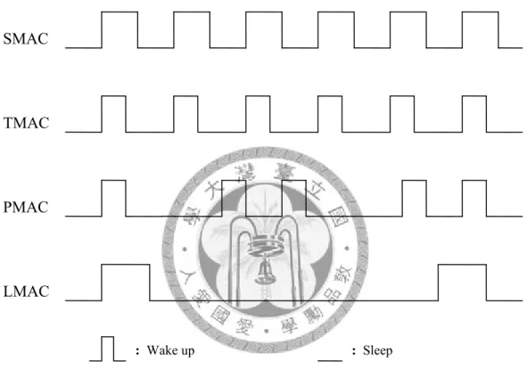
Figure 1 shows the comparisons of wake-up/sleep state between SMAC, TMAC, PMAC, and LMAC. When sensor nodes in LMAC wake up, we try to guarantee there are packets waiting in their children’s buffer to be sent.

One problem of data packet arrival time prediction is that the sensor nodes will suffer some levels of penalty for missing prediction because the protocols will schedule certain operations for this arriving data packet such as self waking up or notifying the next node to be ready to receive this data packet. PMAC generates patterns via the past traffic conditions, but the traffic load might be unstable and cause the patterns to unfit the current traffic. The problem in a fixed-schedule based MAC protocol is when a node wakes up and listens to the medium, there might have no packet incoming or sent out

(19)

from the buffer. In a S-MAC-like protocol, the incoming rate is not considered. Instead, a sensor node wakes up every fixed period to check if there are packets incoming or sent out. What S-MAC can do is nothing but adapting the sleep duty cycle to fit the environment setup.

SMAC

TMAC

PMAC

LMAC

: Wake up : Sleep

Figure 1. Listening State of MAC Protocols

(20)

CHPATER 3

LATENCY MAC

3.1 Overview of Latency MAC

In an extreme case, a sensor node could minimize the energy wastage by sleeping for a very long time and waking up for a short time. It receives all the data from previous nodes and then sends them out in the duration of wake up. Obviously, this method can totally avoid the idle listening wastage but it will cause the data out of date and the buffer overflowing. In LMAC, the scenario is similar. Every sensor node will store a certain number of data packets which are either received from the neighboring nodes or sensed by the sensor node in buffer for a certain time length.

A Poisson process is a sequence of events randomly spaced in time. A Poisson process has the property of independent increments, i.e., it’s timeless and memoryless.

A sensor node will sample the environment periodically, but the sampling data might not be stored in buffer. Therefore, the data arrival in sensor networks can be treated as a Poisson process system. The following data arrival we describe is based on Poisson arrival.

As we describe above, a protocol can predict the arrival time of packets, but the prediction accuracy can not be 100%. In a Poisson arrival system, if the arrival rate is λ, the possibility of n data packets arrival in T time units is n ⁿ e ^λ^T

n T T λ

P  ^

! ) ) (

( . Now we

know the arrival rate is λ and we predict there is an incoming packet every

λ

1 time unit,

the missing rate is P0(

λ

1 ), that is 36%. Once a sleep schedule is generated according to

this prediction then the idle listening will occur every 3 sleep cycles. However, if we

(21)

predict there is at least one incoming packet every λ

2 time unit, the missing rate is 13%.

One of the benefits of extending sleep cycle is that we greatly reduce the energy wastage caused by idle listening but we might suffer the additional data latency.

In LMAC, we also predict the time of incoming packets but we do not take it as a true incoming. Our scheduling goal is to announce the sleep cycle and the transmission number to the neighbors. Every sensor node will calculate two parameters for scheduling: Doze and Bulk. Doze stands for how many time slots a sensor node will sleep. Bulk represents the number of data packets that a sensor node will try to transmit at most after waking up from sleeping. Doze parameter stands for a sensor node will

transmit data packets every Doze time slots. Every sensor node will calculate its own Doze and Bulk according to the Doze and Bulk parameters of the children nodes. After

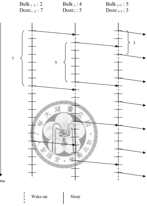
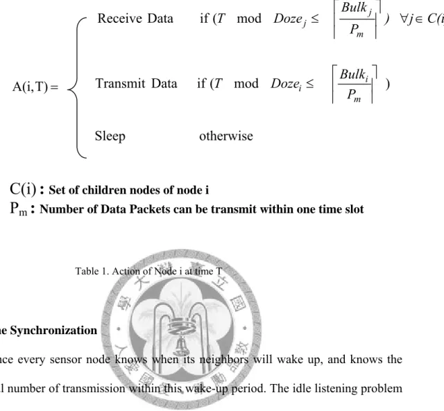
the schedule is generated, every sensor node will transmit at most Bulk data packets every Doze time slots. While a sensor node sleeping within this Doze period, the sensor node will still wake up and receive its children’s data if its children is waking up from the sleeping and ready to send out of data packets. Table 1 shows the action a sensor node i will perform at time T. Pm stands for the maximal number of data packets can be transmit within one time slot. Node i will wake up and receive data when its children j is waking up after sleeping Dozej time slots. And node i will wake up to transmit data to its next node when node i has slept Dozei time slots. A sleep schedule example with Doze parameter is given in figure 2. After the initial schedule has been generated, we can calculate the data latency for this initial schedule and then adjust the schedule to fit the latency constraint.

(22)

Node i-1 Node i Node i+1

Figure 2. Sleep and wake-up states of sensor nodes in LMAC Time

Bulk i -1 : 2 Doze i -1 : 7

Bulk i : 4 Doze i : 5

Bulk i+1 : 5 Doze i+1 : 3

Wake-up Sleep

7 5

3

(23)

3.2 Time Synchronization

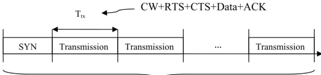
Since every sensor node knows when its neighbors will wake up, and knows the maximal number of transmission within this wake-up period. The idle listening problem has been solved because we increase the possible transmission within each wake-up period. Time synchronization is an unavoidable overhead for TDMA or time slot based MAC protocols. In LMAC, the time synchronization action is performed at the beginning of each active time slot as shown in figure 3. Ttx stands for the time length required to complete a data transmission, including the contention window, RTS, CTS, DATA, and ACK. Except for time synchronization, a sensor node only executes 3 actions in a time slot. A sensor node will either remain in sleep when there is no transmission on schedule or wake up if its previous nodes have transmission on schedule. Receiving and sending transmission can be operated in the same time slot.

C(i) j

) P

Bulk Doze

T

m j

j   



 



  mod

( if Data Receive

T)

A(i, 

^Transmit^Data^if ⁽^T^mod^Doze ^Bulk_P ⁾

m

i i



 



 

otherwise

Sleep

C(i) :

Set of children nodes of node i

P

m

:

Number of Data Packets can be transmit within one time slot

Table 1. Action of Node i at time T

(24)

The number of transmission within one time slot depends on the time unit of arrival rate, network bandwidth, and data packet size.

3.3 Details of Sleep Schedule in LMAC

3.3.1 Bulk and Doze Parameters

In order to achieve the goal we state above, we have to define the algorithm to initiate Doze and Bulk parameters for all sensor nodes. In a Poisson arrival system, the maximal Bulk number of a sensor node is limited by many causes such as buffer size of a sensor node, network bandwidth, data packet size, etc. The Bulk stands for the number of data packets a sensor node will transfer at most within one sleep cycle. As a result, the Bulk number was bounded by the transmission time of each data packet. Doze parameter indicates the sleep time of a sensor node before it sends out data. When a sensor node is sleeping for Doze time length, it will still wake up to receive data there its children nodes are ready to transmit data.

3.3.2 Transmission Rate Constraint

Let Pm be the number of data packets can be transmitted within one time slot A sensor node has to transmit Bulk data packets within the Doze sleep cycles. Since both

Time Slot

SYN Transmission Transmission ^…

Ttx CW+RTS+CTS+Data+ACK

Figure 3. Contents of Time Slot

Transmission

(25)

the receiving and transmitting actions might happen in the same time slot, the expected bandwidth is only half of the bandwidth.

m

k

P

k

oze  2  Bulk

D

₍₁₎

3.3.3 Buffer Overflow Constraint

In a Poisson arrival system, we can not guarantee the buffer is overflow-free no matter how big it is. What we can do is just setting an overflow probability threshold and controlling the overflow probability under this threshold. For a sensor node, the numbers of incoming data from children nodes are determined, so we only have to investigate the relations between the remaining buffer space and self-sensed data packets. Let the buffer size of node k be Bufferk . C(k) stands for all the children nodes connected to node k. The remaining buffer space bk is that Bufferk takes away the maximal possible arrival data within the Dozek sleep cycles. We will calculate the overflow probability with buffer size bk.



 











i k k

k Doze

Doze C(k)

j Bulk j

Buffer

b ₍₂₎

 





 

 ^k ^k ^k

j k k k

b j

Doze e λ

j!

Doze - λ

]) Overflow P([

0

)

1 ( (3)

3.3.4 Latency Constraint

If a sensor network has a data latency restriction, we will consider the latency for the leaf nodes only because the leaf nodes have the largest data latency in all nodes. For a data packet been transmitted to the sink from a leaf node, it will suffer the following latency factors: carrier sense latency, backoff latency, sleep latency, queuing latency,

(26)

and transmission latency [12]. Carrier sense latency indicates that the sensor node performs the carrier sense action. Backoff latency is that when a sensor node fails on carrier sense, it will redo the carrier sense action after a random short time period.

When the sensor node is in sleep, it will not transmit the self-sensed data packet or received immediately. The waiting time between data packet arrival and transmission is sleep latency. The queuing latency indicates the waiting time of a data packet in buffer from beginning transmission to being delivered. The transmission latency is the time required to transmit a packet out and it depends on the network bandwidth. Comparing to other latency factors, carrier sense latency and backoff latency are smaller and we can ignore them.

Let P(k) be a set of nodes including all the ancestor nodes connected to node k, i.e.

all the nodes will pass the data packets which are sensed by node k to sink. The expected latency includes sleep latency, queuing latency, and transmission latency. W(k) is the average queuing time for data packets in Node k.

 



 



   



P(k) i

T T i Bulk

Doze )

E(L_k _i _tx _tx

2 1 2

1 (4)

In order to confront the latency constraint, we should calculate the worst case of latency and use it as the upper bound.

 

   



P(k) i

T T

i Bulk Doze

L_k _i 2 _tx 2 _tx (5)

After the above restrictions are considered, we can finally study the relation between Bulk and Doze. For the node k, Bulkk must be greater than the number of possible arrival data packets within Dozek or the buffer will overflow.



k k



C(k) i

i i

k k Bulk λ Doze

Doze

Bulk Doze  

 



 





 (6)

(27)

If the number of data packets in buffer is less than Bulk, a sensor node can turn off radio and stop everything to sleep after transmitting all the data packets in buffer. On the other hand, if the number of data packets in buffer is greater than Bulk, it has to wait for the next time slot.

3.3.5 Initial Scheduling

After understanding all the restrictions and relations of Bulk and Doze, we can generate an initial schedule for networks. A series graphics in figure 4 has shown the schedule initiate diagram step by step. Firstly, we have every sensor node use its

“following node number” as the initial Bulk number as shown in figure 4(b). Since we have got every node an initial Bulk number, we can calculate its Doze parameter by (6) as shown in figure 4(c). After generating every node’s Doze parameter, we can calculate the latency for the leaf nodes by using formula (5). If the latency has not reached the limit of the system, we will adjust the Doze by (5). After the new Doze parameters are attained, we can re-adjust the Bulk parameters. Then we get a sleep and transmission schedule to fit the latency constraint as shown in figure 4(d). There is one more restriction while setting Doze parameters: when a sensor node’s Doze parameter has been given and adjusted by (5), the next network chain connected to this sensor node can only decrease its Doze parameter but not increase it. This restriction is to prevent the latency of leaf nodes in a network chain be effected by another network chain and caused the packet breaks the latency constraint.

(28)

( 30,3) ( 39,6) ( 15,3)

( 15,3) ( 24,12) ( 24,15) ( 21,24) ( 18,27)

( 15,6) Figure 4(d). Schedule fits Latency Constraint

Sink

( 10,1) ( 13,2) ( 5,1)

( 5,1) ( 8,4) ( 8,5) ( 7,8) ( 6,9)

( 5,2) Figure 4(c). Initial Doze parameters

Sink

( ?,1) ( ?,2) ( ?,1)

( ?,1) ( ?,4) ( ?,5) ( ?,8) ( ?,9)

( ?,2) Figure 4(b). Initial Bulk parameters

Sink

0.05 0.2 0.2

0.2 0.1 0.1 0.1

0.2

0.1

Figure 4(a). Data Arrival Rate Sink

(29)

3.4 Optimization

The scheme we describe above in setting initial Bulk parameters is just one basic option. In a system with a loose latency constraint, we can give some nodes higher initial Bulk numbers in order to optimize the energy-efficiency. There is one more energy-efficiency problem we stated earlier: unbalanced energy consumption. A sensor node closer to the sink will consume more energy than that far away from the sink because the data flow will pass through more frequently. [5] We can slightly reduce the unbalanced energy consumption by giving heavy load sensor node more initial Bulk number.

3.5 Traffic Adaptation

In Latency MAC, we have to know the arrival rate and the latency constraint to generate schedule for every sensor node. After initial and optimal operations, the schedule is fixed and will be performed periodically. If any events happen to this network topology such as sensor nodes running out of battery, sensor nodes’ arrival rate being changed, one of sensor nodes is broken in the middle of the network chain, etc.

What we have to do is just re-scheduling the network chain from the changed nodes to sink. All other nodes does not connect to those changed nodes will not be affected.

However, the energy-efficiency performance of LMAC will decrease and not be optimal anymore.

(30)

CHPATER 4 SIMULATIONS

4.1 Simulation Tool: NS2

The Network Simulator (NS2) [15] is one of the most mature network simulation tools. It is heavily used in ad-hoc research because it supports any array of popular network protocols and offers simulation results on wired and wireless networks.

4.2 Simulation Setup

In our simulation setup, we will focus on energy consumption. We will simulate LMAC, SMAC, and PMAC and compare their performance in different metrics. SMAC is the most popular basic contention based MAC protocol used in wireless sensor network. There are many other MAC protocol designs develop based on SMAC. So we pick it as one of our compare object. PMAC is a traditional data packets arrival prediction MAC protocol. It will suffer idle listening penalty when the prediction is missed. In addition, it has to use more energy to maintain patterns for every sensor nodes while LMAC only generate schedules at the beginning. The simulation topology is a square grid mesh network with different sizes. The other setup parameters are shown in Table. 2. Our simulations will focus on some specific features: total energy consumption on different traffic load, arrival rates, and latency constraints over different numbers of sensor nodes.

(31)

4.3 Simulation Result

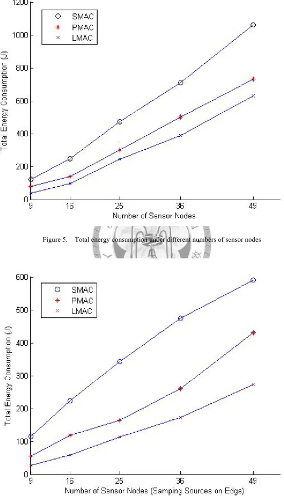
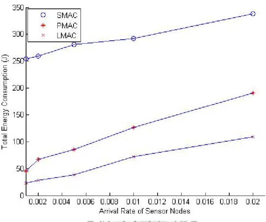
In figure 5, we compared the total energy consumption under different numbers of sensor nodes (average arrival rate 0.05) over a mesh network. In this simulation, there are no certain data sources. Instead, every sensor node will sense data and forward it to the sink. The total energy consumption of LMAC is 28% of that of SMAC when the network size is small. However, when the network size is larger, the total energy consumption of LMAC is 59% of that of SMAC. The difference of energy consumption is smaller because there are too many data packets flowing in the network. Thus, no matter when a sensor node wakes up, there are a lot of data packets ready to be sent in buffer. In figure 6, only the leaf nodes on the left and bottom edges will sense data over a grid network topology. In this setup, we can clearly see that the energy consumption of LMAC is much less than that of SMAC and PMAC. The total energy consumption of LMAC is 23% of that of SMAC and 50% of that of PMAC when the traffic load is small. In figure7, we show that the energy consumption of the busiest sensor node in the network. In figure 8, we show the total energy consumption under different arrival rate.

The energy consumption of LMAC is smaller more when the arrival rate is small. The

Sending Power 0.25 w

Receiving Power 0.2 w

Idle Power 0.1 w

Simulation Time 1000 secs

Poisson Arrival Time Unit 100 ms

Bandwidth 20 kbps

Data Packet Size 20 bytes Parameters of Simulation Environment

Table. 2. Simulation Setup Parameters

(32)

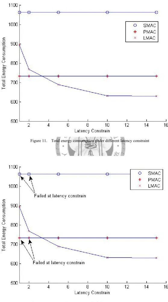
performance difference is more obvious when the source nodes are only leaf nodes on edges. In figure 11, we show the total energy consumption under different latency constraints. LMAC indeed consume less energy when the latency constraint is bigger.

But when the latency constraint is larger than a threshold, the total energy consumption of LMAC is fixed because the idle listening caused by inaccurate prediction no longer exists. Or the other restrictions such as buffer size, transmission rate will bound the minimal energy consumption.

(33)

Figure 5. Total energy consumption under different numbers of sensor nodes

Figure 6. Total energy consumption under different numbers of sensor nodes &

(34)

Figure 8. Total energy consumption under different arrival rates

Figure 7. Energy consumption of the busiest sensor node under different numbers of sensor nodes

(35)

Figure 9. Total energy consumption under different arrival rates & Source nodes on edge

Figure 10. Energy consumption of the busiest sensor node under different arrival rates

(36)

Figure 11. Total energy consumption under different latency constraint

Figure 12. States of latency constraint failures

(37)

PMAC SMAC

9 122.22% 243.43%

16 42.86% 155.82%

25 21.78% 92.73%

36 29.06% 84.18%

49 16.34% 68.73%

LMAC PMAC SMAC

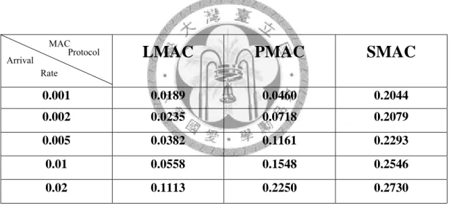
0.001 0.0189 0.0460 0.2044 0.002 0.0235 0.0718 0.2079 0.005 0.0382 0.1161 0.2293 0.01 0.0558 0.1548 0.2546 0.02 0.1113 0.2250 0.2730

Table 3. Extra energy consumption compared to LMAC under different numbers of nodes

MAC Protocol Arrival

Rate

Table 4. Average Energy Consumption per packet under different arrival rates MAC Protocol

Number of Nodes

(38)

CHPATER 5

CONCLUSION AND FUTURE WORK

This paper considers the reasons causing idle listening and tries to avoid them by sacrificing latency to increase the arrival prediction accuracy. LMAC outperforms energy-consumption over SMAC and PMAC under a loose latency constraint and a light traffic load in the wireless sensor network environment. It can operate successfully in the high traffic load and the high latency constraint as well.

In a light traffic load scenario, prediction-based protocols and constant sleep wake- up schedule protocols will suffer more energy wastage penalty from idle listening due to the uncertainty of incoming data. LMAC prevents the uncertainty by increasing the length of sleep cycles to guarantee the existence of transmission when a sensor node wakes up. This method greatly reduces the total energy consumption. Moreover, in a loose latency constraint setup, LMAC can use the extra latency to increase the prediction accuracy while other protocols do not take latency constraint factor into consideration.

The most important future work in LMAC is to initiate Bulk parameter. In chapter 3, we present many initial options of Bulk parameters. However, these initial options for Bulk parameters can only be done manually. These methods try to please some specific

sensor nodes but they can not guarantee the option is optimal for the network topology.

We will try to find an algorithm to give every sensor node a weight that stands for its energy consumption rank.

An improved time synchronization is another work that needs to be done in the future. In LMAC, sensor nodes will sleep for a fixed time slot and then wake up. A

(39)

sensor node which has more than one child does not have the cooperative action of its children. What the children do is to compete for the access of medium. The future work is to solve this problem by either giving sensor nodes a cooperation scheme or trying to stagger the transmission like DMAC.

(40)

CHPATER 6 REFERENCE

[1] Akyildiz, I.F.; Weilian Su; Sankarasubramaniam, Y.; Cayirci, E

“A survey on sensor networks” IEEE Communications Magazine Aug. 2002 [2]G. Lu; B. Krishnamachari; C. Raghavendra

“An Adaptive Energy-Efficient and Low-Latency MAC for Data Gathering in Sensor Networks” International Workshop on Algorithms for Wireless, Mobile, Ad Hoc and Sensor Networks (WMAN 04), April 2004.

[3] Jianfeng Mao; Cassandras, C.G.

“Optimal Control of Two-Stage Discrete Event Systems with Real-Time Constraints”, Discrete Event Systems, 8th International Workshop, 2006

[4] JL Gao

“Analysis of Energy Consumption for Ad Hoc Wireless Sensor Networks Using a Bit- Meter-per-Joule Metric” IPN Progress Report, 2002

[5]M. Stemm; R. H. Katz.

“Measuring and reducing energy consumption of network interfaces in hand-held devices,” IEICE Trans. on Communications. Aug. 1997.

[6] Miller, M.J.; Vaidya, N.H.

“A MAC protocol to reduce sensor network energy consumption using a wakeup radio”

IEEE transaction on Mobile Computing. May. 2005.

[7] Phil Karn.

“MACA-a new channel access method for packet radio” ARRL/CRRL Amateur Radio 9th Computer Networking Conference, 1990

(41)

[8] Prabhakar, B.; Uysal Biyikoglu, E.; El Gamal, A.

“Energy-efficient Transmission over a Wireless Link via Lazy Packet Scheduling”

INFOCOM 2001, Proc. 20th Annual Joint Conf. of the IEEE Computer and Communication Societies.

[9] Shan, R.C.; Rabaey, J.M.

“Energy aware routing for low energy ad hoc sensor networks” WCNC2002. IEEE Wireless Communications and Networking Conf, Mar 2002

[10] T. V. Dam; K. Langendoen

“An Adaptive Energy-Efficient MAC Protocol for Wireless Sensor Networks,”

SenSys’03, Los Angeles, Nov. 2003.

[11] Wei Lai; Paschalidis; Ioannis Ch.

“Routing through noise and sleeping nodes in sensor networks: latency vs. energy tradeoffs” Proceedings of the 45th IEEE Conference on Decision & Control December, 2006 [12] Wei Ye; Heidemann, J.; Estrin, D.

“Medium Access Control With Coordinated Adaptive Sleeping for Wireless Sensor Networks” IEEE/ACM Transactions on Networking. June. 2004

[13] Yang Yu; Krishnamachari, B.; Prasanna, V.K.

“Energy-Latency Tradeoffs for Data Gathering in Wireless Sensor Networks”

INFOCOM 2004. 23th AnnuaJoint Conf. of the IEEE Computer and Communication Societies.

[14] Zheng, T.; Radhakrishnan, S.; Sarangan, V.

“PMAC: An adaptive energy-efficient MAC protocol for Wireless Sensor Networks” in Proc. 19th IEEE International Parallel and Distributed Processing Symposium, 2005.

[15] http://www.isi.edu/nsnam/ns/

[16] http://wushoupong.googlepages.com/ns2scenariosgeneratorchinese

(42)